OPTIMIZING HYDROPATHY SCALE TO IMPROVE IDP PREDICTION AND CHARACTERIZING IDPS’ FUNCTIONS
Fei Huang
Submitted to the faculty of the University Graduate School in partial fulfillment of the requirements
for the degree Doctor of Philosophy
in the Department of Biochemistry and Molecular Biology, Indiana University
Accepted by the Graduate Faculty, Indiana University, in partial fulfillment of the requirements for the degree of Doctor of Philosophy.
A. Keith Dunker, Ph.D., Chair
Jake Chen, Ph.D.
Doctoral Committee
November 19, 2013 Thomas D. Hurley, Ph.D.
Li Shen, Ph.D.
ACKNOWLEDGEMENTS
First and foremost, I would like to express my deepest gratitude to Dr. A. Keith Dunker, for his mentorship and support through my graduate study. Dr. Dunker is a great scientist with knowledge and character. What I have learnt from Dr. Dunker will have a great influence on my future career.
I also would like to thank Dr. Vladimir Uversky. Dr. Uversky gave me valuable advices and guidance for all my research. I am indebted to Dr. Uversky for all the great ideas he came up for my research.
Thank my committee members, Dr. Jake Chen, Dr. Thomas D. Hurley, and Dr. Li Shen. Also thank my former committee members, Dr. Yaoqi Zhou and Dr. Pedro Romero, who have relocated to other Universities. Thank you for the comments and critics, many of which have turned into valuable data for publications.
Thank Chris Oldfield, for all the assistance and discussions on the research, and about life outside.
Thank all the lab members, Bin, Bo, Caron, Eshel, Jingwei, Maya, and Wei-lun. I appreciate your help and support inside and outside of the lab.
Fei Huang
Optimizing Hydropathy Scale to Improve IDP Prediction and Characterizing IDPs’ Functions in PDB Dimers
Intrinsically disordered proteins (IDPs) are flexible proteins without defined 3D structures. Studies show that IDPs are abundant in nature and actively involved in
numerous biological processes. Two crucial subjects in the study of IDPs lie in analyzing IDPs’ functions and identifying them. We thus carried out three projects to better
understand IDPs.
In the 1st project, we propose a method that separates IDPs into different function groups. We used the approach of CH-CDF plot, which is based the combined use of two predictors and subclassifies proteins into 4 groups: structured, mixed, disordered, and rare. Studies show different structural biases for each group. The mixed class has more order-promoting residues and more ordered regions than the disordered class. In addition, the disordered class is highly active in mitosis-related processes among others. Meanwhile, the mixed class is highly associated with signaling pathways, where having both ordered and disordered regions could possibly be important.
The 2nd project is about identifying if an unknown protein is entirely disordered. One of the earliest predictors for this purpose, the charge-hydropathy plot (C-H plot), exploited the charge and hydropathy features of the protein. Not only is this algorithm simple yet powerful, its input parameters, charge and hydropathy, are informative and readily interpretable. We found that using different hydropathy scales significantly
affects the prediction accuracy. Therefore, we sought to identify a new hydropathy scale that optimizes the prediction. This new scale achieves an accuracy of 91%, a significant improvement over the original 79%.
In our 3rd project, we developed a per-residue C-H IDP predictor, in which three hydropathy scales are optimized individually. This is to account for the amino acid composition differences in three regions of a protein sequence (N, C terminus and internal). We then combined them into a single per-residue predictor that achieves an accuracy of 74% for per-residue predictions for proteins containing long IDP regions.
A. Keith Dunker, Ph.D., Chair
TABLE OF CONTENTS
LIST OF TABLES ... viii
LIST OF FIGURES ... ix
LIST OF ABBREVIATIONS ... x
I. INTRODUCTION ... 1
1. Definition of Intrinsically Disordered Proteins (IDPs) ... 1
2. Challenging the protein structure-function dogma ... 2
2.1 protein structure-function dogma ... 2
2.2 Different voices ... 3
2.3 NMR study reveals large disordered regions ... 3
2.4 Computational method reveals amino acid composition bias for IDPs ... 4
3. IDP predictors ... 5
3.1 Early predictors and C-H plot method ... 6
3.2 IUPred ... 7
3.3 PONDR predictors ... 7
3.4 CASP (Critical Assessment of Protein Structure Prediction) ... 9
4. IDP abundance in nature ... 9
5. IDP functions ... 10
5.1 PPI (Protein-Protein Interactions) ... 10
5.2 IDPs in alternative splicing ... 11
5.3 IDPs in transcription factors ... 12
6. Study goals ... 13
II. MATERIALS AND METHODS ... 14
1. Subclassifying disordered protein by the CH-CDF plot method... 14
1.1 Protein data ... 14
1.2 PDB Coverage ... 14
1.3 GO term analysis ... 14
2. Optimizing IDP-Hydropathy Scale for Disorder Prediction ... 15
2.1 Dataset ... 15
2.2 Benchmarking scales ... 16
2.3 Dealing with unbalanced data ... 16
2.3.1 Assessment metrics ... 16 2.3.2 Training method ... 19 2.4 Correlation study ... 20 2.5 Benchmarking ... 20 2.6 Charge-Hydropathy plots ... 21 2.7 Heat map ... 21
3. Per-residue Charge-Hydropathy Disorder Prediction ... 22
3.1 Dataset ... 22
3.2 Disorder distribution along the sequence ... 23
3.3 Correlation of amino acid composition at different regions ... 23
3.4 Training via linear SVM ... 23
III. RESULTS ... 25
1. Subclassifying disordered protein by the CH-CDF plot method... 25
1.1 CH-CDF plot ... 27 vi
1.2 PDB coverage ... 30
1.3 Sequence window CH-CDF analysis ... 36
1.4 Match PDB coverage to disorder prediction ... 38
1.5 Function analysis for each quadrant ... 41
1.6 Discussion ... 43
1.7 Structural Partitioning by the CH-CDF plot ... 43
1.8 The rare protein quadrant (Q1)... 45
1.9 Disorder subtypes and IDP functions ... 46
1.10 Summary ... 47
2. IDP hydropathy: A New Scale That Optimizes Disorder Prediction... 48
2.1 Background and motivations ... 48
2.1.1 Protein folding, the hydrophobic effect, and disorder prediction ... 49
2.1.2 Various hydropathy scales ... 49
2.2 Comparing Hydropathy scale of Kyte & Doolittle (1982) ... 51
2.3 Finding the optimal hydropathy scale for IDP prediction ... 54
2.3.1 Use of Linear SVMs to find hydropathy scales ... 54
2.3.2 Choosing window size for training ... 56
2.4 Disorder is harder to predict ... 61
2.5 Benchmark ... 64
2.6 Correlation study ... 70
2.7 Heat map and values of IDP-Hydropathy versus other scales ... 72
2.8 Comparing C-H plots from different hydropathy scales ... 76
2.9 Discussion ... 86
2.9.1 Disorder is harder to predict ... 87
2.9.2 Error analysis ... 87
2.9.3 Limitations of composition based IDP predictors ... 90
2.9.4 Application and future work ... 90
2.10 Summary ... 91
3. Per-residue Charge-Hydropathy Disorder Prediction ... 92
3.1 Disorder is not evenly distributed alone the sequence ... 94
3.1.1 Disorder is enriched at the N/C terminus ... 94
3.1.2 Disorder composition difference ... 96
3.2 Optimizing hydropathy scale for improved disorder prediction ... 100
3.3 Benchmark the per-residue IDP scale ... 104
3.4 Further improvements ... 106
3.5 Summary ... 107
REFERENCES ... 108 CURRICULUM VITAE
LIST OF TABLES Table 1 ... 37 Table 2 ... 42 Table 3 ... 53 Table 4 ... 60 Table 5 ... 63 Table 6 ... 65 Table 7 ... 67 Table 8 ... 71 Table 9 ... 74 Table 10 ... 89 Table 11 ... 98 Table 12 ... 101 viii
LIST OF FIGURES Figure 1 ... 29 Figure 2 ... 31 Figure 3 ... 33 Figure 4 ... 35 Figure 5 ... 39 Figure 6 ... 58 Figure 7 ... 69 Figure 8 ... 75 Figure 9 ... 78 Figure 10 ... 81 Figure 11 ... 95 Figure 12 ... 99 Figure 13 ... 103 Figure 14 ... 105 ix
LIST OF ABBREVIATIONS
IDP Intrinsically Disordered Protein PDB Protein Data Bank
NMR Nuclear magnetic resonance CD Circular Dichroism
PONDR Predictors of Natural Disordered Regions
VSL2 Variously Characterized Short and Long Regions, Version 2 PSSM Position-Specific Scoring Matrix
CASP Critical Assessment of Protein Structure Prediction PPI Protein-Protein Interactions
MoRF Molecular Recognition Feature
HOX Homeotic
Exd Extradentical
MCC Matthews Correlation Coefficient NPV Negative Predictive Value
ROC Receiver Operating Characteristic
CH Charge-Hydropathy
CDF Cumulative Distribution Function AAindex Amino Acid Index Database SVM Support Vector Machine
Trx Thioredoxin
PPV Positive Predictive Value
AUC Area Under Curve
I. INTRODUCTION
1. Definition of Intrinsically Disordered Proteins (IDPs)
Intrinsically Disordered Proteins (IDPs) are proteins without defined 3D structures1–5. ‘Disorder’ describes the lack of structure of such proteins. The term
‘intrinsically’ means that their failure to fold into a specific 3D structure is inherent in the amino acid sequence6,7; i.e., encoded by their amino acid sequences. It is important to note that the amino acid composition of IDPs is biased towards certain amino acids, compared to the compositions of ordered proteins4.
Many other expressions are used to describe these proteins as well. Commonly known expressions are, floppy, pliable, rheomorphic, flexible, mobile, partially folded, natively denatured, natively unfolded, natively disordered, intrinsically unfolded,
vulnerable, chameleon, malleable, 4D, protein clouds, dancing proteins, proteins waiting for partners, and others6. These terms were proposed by many researchers when they encountered IDPs during their research, and found that these proteins exhibit features distinguishable from those of globular proteins.
Despite the differences in the use of words, almost all of these names suggest a common feature, flexibility. However, flexibility is not stringent enough to be an appropriate descriptor for these proteins. Many structured proteins, such as the binding pocket of an enzyme, may have some degrees of flexibility but they are not IDPs6. Protein ensembles with no preferred lowest energy conformation that adopt many different forms, is a more accurate description8. Thus, we use the term ‘disorder’ to define this state of these proteins.
Even though not illustrated in all of the terms, some researchers used names that included words such as ‘natively’ or ‘naturally’. The word ‘intrinsically’ was chosen in the end because it illustrates the two most important features of these proteins equally well: 1. disorder is inherently encoded in their amino acid sequences; 2. the state of disorder is manifested under generic physiological conditions6.
In contrast, ‘ordered’ or ‘structured’ proteins indicate proteins that have a preferred lowest energy conformation, i.e., a well-defined 3D structure. Therefore, the term ‘disordered’ and ‘ordered or structured’ are adopted throughout this manuscript to indicate proteins that are not disordered. It is worth noting that many proteins possess both states, with each state in different regions of the sequence. We refer to these proteins as ‘partially disordered or partially ordered proteins’, and we name these regions as ‘disordered or ordered regions’.
2. Challenging the protein structure-function dogma 2.1 protein structure-function dogma
The study of IDPs has been of growing interest in the recent years9,10. However, it is not always this case from the beginning. For a long time, the idea that a protein can carry out function without folding into 3D structure was not recognized by the scientific community9.
The proteins structure-function dogma has been dominant for a long time. In 1894, Emil Fischer made the astonishing discovery of enzyme specificity. He therefore
proposed the ‘lock and key’ model to explain such strong specificity11. In 1931, Hsien Wu proposed that loss of function via protein denaturation occurred when weak
interactions were disrupted leading to loss of structure12. This paradigm, that structure is necessary for function, became dominant following the very large numbers of protein structures determined by X-ray crystallography13. To date, 94813 protein structures haven been determined and deposited in the Protein Data Bank (PDB)14.
2.2 Different voices
During that time, however, there were examples suggesting that this dogma was not perfect. In 1953, scientists made the observation that milk protein casein is likely to be unstructured and this might help infants’ digestion15,16. As reviewed by Sigler17, in the 1980s several researchers found that eukaryotic transcription factors have large regions of highly unusual sequences with high content of acidic residues, termed as ‘acid blobs’ or ‘negative noodles’. These regions fail to fold into 3D structures, yet they carry out gene regulation.
However, these examples are sparse and failed to draw wide attention. They were merely considered to be rare exceptions to the dogma. The traditional view of protein structure-function dogma still held its place until the late 1990s, when nuclear magnetic resonance (NMR) and bioinformatics study of IDPs blossomed18–20.
2.3 NMR study reveals large disordered regions
Unlike X-ray crystallization, NMR method to study protein conformation does not require crystallization. NMR thus is more suitable to study IDPs20. Because of IDPs’ lack of stable conformation, their NMR spectra yield multiple very different structural possibilities. Human cell cycle control protein p21 was shown by NMR to be entirely
disordered, and its regulatory functions were shown to depend on its disordered state21. So far, many proteins are confirmed to be disordered or having a long disordered region, where “long” is generally taken to be ≥ 30 residues 20,22–32. Besides NMR, missing sequences in X-ray structure19,33–35, Raman optical activity36, Circular Dichroism (CD)37– 40
, and protease sensitivity experiments41 can also identify IDPs. Since each method has uncertainties with regard to IDP characterization, it would be an advantage to use multiple methods for IDP characterization in which case the different methods complement each other42.
2.4 Computational method reveals amino acid composition bias for IDPs
When more and more experimental data about disordered protein accumulated, people started to ask the question why IDPs do not fold. Bioinformatics study of IDPs’ composition reveals that IDPs have their own preference of amino acid residues
compared to ordered proteins4,43–46. In general, hydrophilic or polar residues are disorder promoting. However, note that additional factors can also influence the disorder/order state of a protein or region as well, such as net charge, aromatic content, side-chain bulkiness, etc.
The folding of an ordered protein is usually driven by the hydrophobic amino acid residues, such as valine, isoleucine, leucine, phenylalanine, methionine, and tryptophan, to form a hydrophobic core. In contrast, a disordered protein usually maintains its
disordered state as a result of its high content of polar residues – i.e., arginine, glutamine, serine, glutamate, and lysine – all of which readily interact with water molecules. Note that cysteine, despite being a polar residue, is missing from the above list. This is because
when oxidized, cysteines greatly promote protein conformation stability by forming disulfide bonds47,48. Cysteine also readily binds prosthetic groups, and thus stabilizes protein structure. Note that even though lysine could also bind to prosthetic groups, it is still a disorder promoting residue because of the charge it carries. Another interesting case here is proline. Although non-polar, proline is a very potent disorder promoting residue. With its unusual secondary amine or imine structure in which the N-H group is replaced with an N-C bond, proline lacks the N-H group critical to alpha-helix or sheet formation and thus is a ‘structure breaker’ that often flanks alpha-helices and beta-sheets49. Overall, compared to strcutred proteins, IDPs are significantly enriched in P, E, S, Q and K.
3. IDP predictors
Many experimental methods are available nowadays to characterize IDPs. However, the number of determined protein sequences is so large that applying experimental method to every one of them is unrealistic. Thanks to the advances in computational biology methods, we can predict the disorder state of a protein or a protein region with fair accuracy by means of supervised learning algorithms.
In particular, given a set of labeled training data, supervised learning algorithm identifies a ‘pattern’ and applies this ‘pattern’ to new data to infer its label50. Given the amino acid compositional differences between structured proteins and IDPs, we can develop algorithms that predict the disordered or ordered state of a protein or region by using amino acid sequences as inputs4,43,51.
3.1 Early predictors and C-H plot method
Currently, many IDP prediction algorithms have been developed4,44,51–55. The first IDP predictor was developed by R.J.P Williams in 197956. Observing that IDPs having abnormally high ratio of number of charged residues divided by the number of
hydrophobic residues, his algorithm separated two IDPs from a set of ordered proteins. The two proteins he studied were from the ribosome and so had a very high net charge. In this case, the high number of charged residues provides more repulsion among amino acids, and thus makes the protein less likely to fold in the absence of RNA. Furthermore, the low number of hydrophobic residues renders less driving force to fold into a
hydrophobic core. However, this method developed in 1978 does not work well for proteins that have a large number of charged groups having a nearly equal balance of positive and negative charges. In this case, the large Williams ratio predicts disorder for many well folded proteins and thus has a very poor acccuracy9.
In 2000, without knowledge of the prior work by Williams, Uversky et al used normalized net charge, not the total charge, and normalized hydrophobicity calculated from Kyte-Doolittle scale4,57 to classify proteins as structured or as natively unfolded. Applying this method to a large number of proteins, including 91 IDPs and 275 ordered proteins gave excellent results4. In 2004, Sussman et al transformed this method to
FoldIndex, a per-residue predictor that can be applied to predict disorder on a local region of protein58. However, FoldIndex did not re-train the data to obtain a new separating function, and the per-residue accuracy of FoldIndex was not evaluated. In fact,
subsequent study shows that the amino acid composition of local disordered regions from partially disordered proteins different significantly from entirely disordered proteins54,55.
As we will show herein, a simple adoption of the original linear function trained with fully disordered proteins performs poorly on partially disordered proteins.
3.2 IUPred
Another biophysical feature based predictor is IUPred, developed by Dosztányi et al. IUPred partitions disordered/ordered proteins by estimating their folding energies52. Without the knowledge of a protein’s 3D structure, IUPred estimates the per-residue energy by assuming that the energy contribution of that residue depends on its amino acid type and potential partners in that sequence. They tried various pairwise sidechain
interaction energy matrices to find the one that gave the clearest difference between the folding energies of structured and disordered proteins estimated by this method. Since disordered proteins and ordered proteins gives different folding energy estimates by this method, IUPred can predict IDPs from the approximated per-residue folding energy.
3.3 PONDR predictors
As discussed above, charge and hydropathy are not the only features having an impact on the disorder/order state of a protein. Other features, including aromatic content, sequence complexity and many others also determine if a protein/region folds or not4,53– 55,59
. In addition, a per-residue predictor that predicts local region disorder is more informative to infer the function of a protein.
PONDRs (predictors of natural disordered regions) are designed as per-residue predictors with a combination of amino acid sequence features54,59,60. The second generation of PONDR, namely VLXT, was a merged neural network of three
predictors61. One predictor was trained on variously characterized, long regions of internal disorder (VL), and the other was trained on X-ray characterized, disordered N or C termini (XT). This predictor achieved a balanced accuracy above 70%, a value
significantly better than the 50% expected by chance for two state prediction on balanced data61.
Later, amino acid composition study on short (<30 residues) and long (>30 residues) disordered regions shows that short and long disordered regions have
significantly different amino acid biases55. VSL2 (variously characterized short and long regions, version 2) was developed to better cope with this difference54. Basically, VSL2 is a meta-predictor of two sub-predictors, one trained with short and the other trained with long disordered regions data. This predictor used evolutionary information obtained by generating the position-specific scoring matrix (PSSM) of the query sequence by PSI-BLAST (Position-Specific Iterated PSI-BLAST)62. However, PSI-BLAST is time consuming. As a result, VSL2B, a much faster ‘light’ version without employing PSSM, is commonly used and achieves an accuracy that is only slightly diminished54.
In 2010, a consensus predictor, PONDER-FIT, was developed59. PONDR-FIT is a neural network meta-predictor based on the outputs of 6 commonly used disorder
predictors, PONDR-VSL254, PONDR-VL363, FoldIndex58, IUPred52, and TopIDP49. The outputs of these 6 predictors are then combined into a single predictor using a neural network. Compared to the best of its 6 individual predictors, PONDR-FIT shows an overall 11% improvement.
3.4 CASP (Critical Assessment of Protein Structure Prediction)
In 2002 CASP5 included disorder predictions with published evaluations, and links to several of these predictors are now available in the DisProt Database
(http://www.DisProt.org)64–67. Note that CASP targets are results of up-to-date experiments and selected so that no prior information about them is revealed to any participants. The biannual CASP experiments serves as excellent, unbiased
benchmarking for various IDP predictors.
However, the CASP disorder prediction experiment provides very unbalanced datasets for which, the number of ordered residues overwhelms disordered residues66,68. Also, the disorder predictions accuracies from recent CASP fluctuate, showing no significant improvement. These fluctuations are likely due to changes in the difficulties presented by the different targets, rather than fluctuations in predictor accuracies66–68. 4. IDP abundance in nature
One application of IDP prediction is to evaluate the abundance of IDP in nature. IDP predictors haven been applied to proteomics dataset of various species35,69–71. In general, disorder is estimated to be much more prevalent in sequence databases and in various proteomes as compared to PDB. Eukaryotes protein sequences contain much more disorder (~33% - 50%) than prokaryotes (~15% - ~30%) and archaea (~12% - ~24%). Such predictions suggest that the human proteome, in particular, contains ~35% - 50% disordered residues70,71. An important, open question is whether the predicted regions of disorder remain disordered inside the cell or become structured upon association with partners or ligands.
5. IDP functions
Given such abundance, one cannot help but wonder what are the functions of IDPs? Also, why do eukaryotes have much more predicted disorder than common bacteria or archaea bacteria?
5.1 PPI (Protein-Protein Interactions)
One of the signature function of disordered protein is carried out through
Molecular Recognition Features (MoRFs)72–76. These MoRFs are typically hydrophobic patches within a disordered region. Upon binding, the hydrophobic groups become buried and the IDP segment typically undergoes a disorder-order transitions. In some cases, significant sized parts of the original IDP region remain unstructured yet contribute to the binding affinity even while remaining unstructured. Interactions involving IDP regions that contribute to binding affinity have been called ‘fuzzy complexes’77,78.
Eukaryotic PPI networks are scale-free, a term that means a plot of the log of the number of nodes versus the log of the number of partners per node gives a straight line. Such a plot means that a few proteins in the network interact with many partners while most proteins interact with only a few partners79–81. Such proteins with high number of binding partners are referred to as ‘hub proteins’. An often-cited analogous network is that provided by the set of airline routes, in which some big cities such as New York or Los Angles contain connecting airports for smaller cities.
It is intriguing to imagine how single proteins can bind to many partners. We suggested that the flexibility of IDPs might provide the key feature that enables one protein to bind to many partners, and we found that a number of hub proteins indeed used
disordered regions to bind to many partners2,21,82,83. Two IDP-based mechanisms were observed for the multipartner binding of hub proteins. In the first mechanism, one disordered region binds to many partners, or ‘one-to-many binding’. In the second mechanism, many disordered regions bind to one partner or ‘many-to-one
binding’2,21,82,83.
The one-to-many binding IDP regions of a hub protein are either in very close vicinity or at the exact same site83. When the same IDP region binds to multiple partners, this IDP region often changes its shape to fit with its different partners. For example, the N-terminal and C-terminal IDP regions of p53 each bind to more than 40 different partners by this mechanism.
Alternatively, many different disordered proteins/regions of different amino acid sequences can bind to a single ordered partner84. Many such examples are found in PDB, in which a single IDP contains two or even three separate MoRF regions binding to the same structured partner.
5.2 IDPs in alternative splicing
Confirmed by both experimental data and computational predicted data,
alternatively spliced protein isoforms are enriched of disordered residues85–87. During the process of many tissue-specific alternative splicing, many MoRF containing IDP region could be either kept or spliced out, resulting in tissue-specific protein-protein interactions based on differential retention of IDP binding regions or MoRFs.
5.3 IDPs in transcription factors
Eukaryotic transcription factors have a high content of disordered residues88,89. The activation domains of transcription factors are often composed of IDPs. Also, structured functional domains in transcription factors are frequently flanked by disordered residues that regulate their binding to DNA.
As an example, HOX (homeotic) domain of Drosphila regulatory transcription factor Ubx is flanked by evolutionarily conserved disordered regions90,91. Alone without the IDP region, HOX domain binds DNA with much higher affinity. In addition, an IDP linked YPWM motif can further weakens HOX binding. To enhance its HOX domain binding affinity, Ubx interacts with Extradentical (Exd). Upon interaction, the IDP linked YPWM motif binds into a pocket of the HOX domain on Exd. Furthermore, the IDP linker between HOX domain and the YPWM motif can be alternatively spliced for different length. Therefore, we speculate that, by regulating the length of the IDP linker and the availability of surrounding Exd’s binding sites, the binding affinity of Ubx’s HOX domain can be either promoted or repressed.
Besides the examples discussed above, IDPs are involved in many more
biological processes, such as protein-RNA interactions92–96, allosteric regulations97–103, chaperone functions104–107, protein evolution108,109, and so on. Through their dynamic features, IDPs participate in numerous biological functions through all kinds of
mechanisms. It is by the dual existence of disorder and ordered state in proteins, proteins can perform wide diversity of functions and become the building blocks of life.
6. Study goals
IDPs are abundant in nature, and they play important roles in many biological processes. Understanding their functions and identifying them are the two major tasks in the study of IDPs. Here, we present two approaches, CH-CDF plot and improved C-H plot method to address these two tasks, respectively.
The CH-CDF plot method is a clustering tool that partitions IDPs into three subgroups. This partition method clusters IDPs according to their biophysical characters. Indeed, each IDP subgroup is shown to have distinguishable function features related to the biophysical features of that group.
To address the 2nd task, we improved the original C-H plot disorder predictor developed by Uversky et al. We optimized the hydropathy scale used to calculate the hydropathy in the original method. The prediction power of C-H plot is significantly improved by the newly developed scales. In addition, this scale is highly correlated with popular hydropathy scales, and thus can be used to calculate hydropathy for better understanding of protein functions.
II. MATERIALS AND METHODS
1. Subclassifying disordered protein by the CH-CDF plot method 1.1 Protein data
The Mus. musculus proteome were gathered from Uniprot 15.055. A total number of 58881 sequences were obtained. Blastclust
(http://www.ncbi.nlm.nih.gov/Web/Newsltr/Spring04/ blast lab.html) with default settings was used to reduce redundancy.
1.2 PDB Coverage
PDB monomers data is downloaded from PDBe PISA. The gapped-BLAST algorithm was used to compare query sequences to PDB monomers, with the default scoring matrix (BLOSUM 62). A hit was identified only when the hit region is larger than 85% of the PDB monomer sequence, and with more than 30% identity.
1.3 GO term analysis
We downloaded GO terms associated with each protein from GO Database. To reduce protein redundancy, proteins were clustered into protein families by Blastclust program. If sequence si was assigned to clusterc(si), and ni is the total number of
proteins assigned to this family, we define a weight w(si) for this sequence as
i i
n s
w( )= 1 .
Our 509,214 proteins are in association with 10,703 GO annotations. Protein sequence si
grouped into a quadrant k, =1, 2, 3, 4 as groupk gk. And forGOj,j=1, 2, … , 10723
there is a cluster of proteins related toGOj, asCj,j=1, 2, … , 10723. Therefore, we
calculatenj,k, the number of proteins related to GOjin quadrant k by j k i i k j w s s g C n, =∑ ( ), ∈ ∩ .
In the next step, we comparenj,1,,nj,2,,nj,3and nj,4for every specific GO term GOjto
examine if GOj has any bias towards a certain quadrant. The expected value of protein
frequency in quadrant kis calculated as
∑
= ⋅ = 4 1 , , k k j k k j p n
E , with pkbeing the proportion of
numbers of proteins in quadrantk. Then we compute 2 j
X , sum of expectancy, as . 2
j
X follows a chi-square distribution with 3 degrees of freedom, 2
j
X ~ χ2(3).
Under the null hypothesis that GOjdistributed in 4 quadrants according to
expectancy, we can derive pjas a p-value forGOj. Since multiple statistical tests are
applied, we use Bonferroni correction to adjust obtained p-value. This correction reduces the scale of significant results as well. A threshold of 0.05 is chosen, and GO terms with p-values less than 0.05 are collected.
2. Optimizing IDP-Hydropathy Scale for Disorder Prediction 2.1 Dataset
Two sets of proteins were used in this study59,60: experimentally verified entirely disordered proteins and experimentally verified completely structured or ordered proteins. Entirely disordered proteins were taken from Disprot 6.064,42. These proteins were filtered such that only those proteins with their entire sequences being disordered were retained. Our fully disordered protein dataset contains 109 disordered sequences with 22,614 amino acid residues. The set of fully structured (ordered) proteins consisting only of
k j k j k k j j O E E X , 2 , 4 1 , 2 / ) ( − =
∑
= 15single-chain and non-membrane proteins was assembled from the Protein Data Bank (PDB)14 (http://www.rcsb.org/pdb/). Only structures determined by X-ray crystallography and characterized by unit cells with primitive space groups were kept in our dataset. Structures with ligands, disulfide bonds, or missing residues were also removed. Then a BLASTCLUST62 analysis was performed to cluster proteins into subsets, with all members of each subset having at least 25% sequence identity with another subset member and having less than 25% sequence identity with any member of any other subset. The longest sequence in each cluster was selected to construct the fully ordered protein set. This set of experimentally determined structured proteins contains 563 fully structured protein sequences with 113,895 amino acid residues.
2.2 Benchmarking scales
We obtained 19 hydropathy scales57,110–127 from ExPASy-ProtScale to compare with the hydropathy scale of Kyte & Doolittle (1982)57. A more thorough benchmarking against various amino acid indices was carried out later with 535 amino acid scales. Among these, 531 amino acid scales were obtained from the Amino Acid index database (AAindex: www.genome.jp/aaindex)128–130. Another 4 disorder propensity scales were also examined, including TOP-IDP49, FoldUnfold131, B-value132, and DisProt49,64,42,133.
2.3 Dealing with unbalanced data 2.3.1 Assessment metrics
Our dataset of disordered/structured proteins is highly imbalanced with 16.2% disordered and 83.8% structured based on numbers of chains or 17% disordered and 83%
structured based on numbers of amino acid residues. Accuracy, defined as the proportion of correctly classified samples in the population (Eq. 1), is not a good measurement when the number of one class dominates134. In fact, simply predicting every case as structured would yield an apparent accuracy close to 0.84. A better approach is to average the correct prediction of order and the correct prediction of disorder, called the balanced accuracy and calculated as follows: first, estimate the value for the correct prediction of disorder, called sensitivity (Eq. 2), and the value for the correct prediction of structure, called specificity (Eq. 3), then average the values for sensitivity and specificity134 (Eq. 4):
𝐴𝑐𝑐= 𝑇𝑃+𝑇𝑁+𝐹𝑃+𝐹𝑁𝑇𝑃+𝑇𝑁 (Equation 1),
where Acc = accuracy, TP = true positive predictions, TN = true negative predictions, FP = false positive predictions, and FN = false negative predictions,
𝑆𝑒𝑒𝑌𝑌𝑠𝑖𝑡𝑖𝑣𝑖𝑡𝑦 (𝑅𝑒𝑒𝑐𝑎𝑙𝑙) =𝑇𝑃+𝐹𝑁𝑇𝑃 (Equation 2),
𝑆𝐶𝐶𝑒𝑒𝑐𝑖𝑓𝑖𝑐𝑖𝑡𝑦= 𝑇𝑁+𝐹𝑃𝑇𝑁 (Equation 3),
𝐵𝑎𝑙𝑎𝑌𝑌𝑐𝑒𝑒𝑑𝐴𝑐𝑐= 𝑆𝑒𝑛𝑛𝑠𝑖𝑡𝑖𝑣𝑖𝑡𝑦+𝑆𝑝𝑒𝑐𝑓𝑖𝑐𝑖𝑡𝑦2 (Equation 4).
The usefulness of the balanced accuracy metric is undermined by the high fraction of structured residues in the training set. That is, predicting more disordered residues
rewards sensitivity much more than the penalty in specificity, so this imbalance
encourages overpredicting disorder66,68,134. To further help with the analysis of prediction on imbalanced data, the positive predictive value (PPV) metric was introduced135–137. PPV, also called “precision”, is calculated as the fraction of correctly predicted disorder versus all the predicted disorder (Eq. 5):
𝑃𝑃𝑉 (𝑃𝑒𝑒𝑒𝑒𝑐𝑖𝑠𝑖𝐶𝐶𝑌𝑌) =𝑇𝑃+𝐹𝑃𝑇𝑃 (Equation 5).
Overpredicting disorder will result in low PPV, whereas a high PPV value indicates that a high proportion of the predicted disorder is indeed actual disorder. Combing PPV with sensitivity (also known as recall) as indicated (Eq.6) yields the F-score, which is an effective representation of the predictive power in imbalanced dataset138:
𝐹 = 2∙𝑝𝑟𝑒𝑐𝑖𝑠𝑖𝑜𝑛𝑛+𝑟𝑒𝑐𝑎𝑙𝑙𝑝𝑟𝑒𝑐𝑖𝑠𝑖𝑜𝑛𝑛∙𝑟𝑒𝑐𝑎𝑙𝑙 (Equation 6).
The F-score values range from 0 to 1, and because of the product of precision and sensitivity in the numerator, a high F-score usually means a high score for both PPV and sensitivity, or recall.
The Matthews correlation coefficient (MCC) is another very commonly used and effective metric for imbalanced datasets66,139 (Eq. 7):
𝑀𝐶𝐶𝐶𝐶 =�(𝑇𝑃+𝐹𝑃)(𝑇𝑃+𝐹𝑁𝑇𝑃∙𝑇𝑁−𝐹𝑃∙𝐹𝑁)(𝑇𝑁+𝐹𝑃)(𝑇𝑁+𝐹𝑁) (Equation 7). 18
The MCC has been observed to be highly correlated with the F-score for disorder prediction in Critical Assessment of protein Structure Prediction 9 (CASP9)66.
In contrast to PPV, a negative predictive value (NPV) measures the correctly predicted structured proteins over all of the predicted structured proteins135 (Eq. 8):
𝑁𝑃𝑉=𝑇𝑁+𝐹𝑁𝑇𝑁 (Equation 8).
A Receiver Operating Characteristic (ROC) curve is a plot of sensitivity versus specificity140. The area under the curve (AUC) is another often used metric for judging predictive power of an algorithm.
Given all of the above, we estimated F-score, MCC, sensitivity, specificity, AUC, PPV, and NPV as the metrics to assess the quality of the predictions that were made on the unbalanced dataset used herein. Sensitivity, specificity and AUC are informative about the correctly predicted disorder and structure of one class. PPV and NPV reveal whether the algorithm is overpredicting disorder or structure. In the end, the F-score and MCC give an overall estimate of the quality of the predictions.
2.3.2 Training method
In the current dataset, disordered proteins are outnumbered and under-represented. To develop a good predictor in the scenario of unbalanced dataset, we tried several
popular methods134. Both under-sampling structured proteins, and oversampling disordered proteins141–143 were implemented separately to achieve a balanced
disorder/order dataset. Synthesizing new data for the disordered class were also carried out to obtain more disordered samples144,145. We found that in this study, all of these methods gave similar results. The approach of adding weights to the SVM cost function134,146,147 so that a greater penalty occurs when a disordered protein is
misclassified, achieves results similar to the sampling methods above while being much simpler to implement compared to under- or oversampling. Therefore, for simplicity, here we only used the approach of using a weighted cost function.
2.4 Correlation study
The absolute value of Pearson product-moment correlation coefficient148, r, was calculated between IDP-Hydropathy scale and each of the 513 scales from AAIndex. For each scale from AAIndex, the correlation of it with IDP-Hydropathy scale is calculated as in Equation 9, where 𝐼𝐷𝑃𝑖 is the score for ith amino acid in IDP-Hydropathy scale,
𝑆𝑐𝑎𝑙𝑒𝑒𝑖 is the score for ith amino acid in that AAIndex. 𝐼𝐷𝑃 and 𝑆𝑐𝑎𝑙𝑒𝑒 stands for the
mean value of the two scales:
𝑒𝑒= ∑20𝑖=1(𝐼𝐷𝑃𝑖−𝐼𝐷𝑃)(𝑆𝑐𝑎𝑙𝑒𝑖−𝑆𝑐𝑎𝑙𝑒)
�∑20(𝐼𝐷𝑃𝑖−𝐼𝐷𝑃)2
𝑖=1 ∙�∑20𝑖=1(𝑆𝑐𝑎𝑙𝑒𝑖−𝑆𝑐𝑎𝑙𝑒)2
(Equation 9).
2.5 Benchmarking
The IDP-Hydropathy scale was derived from windows of proteins. Since entire protein sequences are applied to the original C-H plot by Uversky et al, for consistency, the benchmarking of IDP-Hydropathy scale and other 554 scales was carried out over the entire protein sequences. The normalized composition and net charge were calculated as
before. Then we obtained the ‘hydropathy score’ for each protein by multiplying the composition matrix and the column vector of the scale. Therefore, 2 attributes are calculated for each amino acid sequences, the ‘hydropathy score’ and the net charge. A linear SVM classifier was then applied to predict disorder/structure proteins.
2.6 Charge-Hydropathy plots
C-H plots were generated using our dataset with the following scales: IDP-Hydropathy, the Guy scale110, and the Kyte-Doolitte (1982) scale57. The normalized net charge was calculated as previously: the absolute value of [(Arginine + Lysine) –
(Glutamate + Aspartate)]/Protein Length. Then the normalized hydropathy was calculated using the indicated scales. Note that to be consistent with the original C-H plot4, the various hydropathy scales were renormalized so as to cover the range between 0 and +1 rather than –1 to +1 as we use elsewhere herein. The linear SVM method implemented by LIBLINEAR library81 was then applied to calculate the boundary in MATLAB
(MATLAB 2012a. Natick, Massachusetts: The MathWorks Inc., 2012).
2.7 Heat map
To provide a visual comparison of variations in the different scales, a heat map was used. The heat map of IDP-Hydropathy and 9 other benchmark scales are drawn by MATLAB HeatMap function (MATLAB 2012a). The scales visualized within the heat map are all normalized to be within –1 and +1. Some of the scales are negatively correlated, so we multiplied them by –1.
3. Per-residue Charge-Hydropathy Disorder Prediction 3.1 Dataset
The data used to train the predictor is downloaded from Protein Data Bank (PDB) and Disprot. PDB data are filtered to discard structures determined by methods other than X-ray structure. PDB data with resolutions lower than 2.5, or structure sequence less than 40 amino acid residues are also discarded. Then, the PDB data and Disprot data are integrated and clustered by BLASTCLUST with 30% identity. The residues in PDB dataset with missing coordinates and residues in Disprot annotated as disordered are considered as disordered amino acid residues. All others are considered as ordered residues. Note that all sequences are extracted as they are in each database. Expression tags such as His-tags and initiating methionine(s) are included.
To pick the sequence from each cluster family, we used the following prioritized criteria as Zhang et al 2012: 1) the sequence with the largest number of disordered residues; 2) sequence with the fewest number of disordered regions (to obtain more contiguous regions of disorder); and 3) protein sequence with the largest length. In the end, we obtained 1619 protein sequences.
As shown in Peng et al 2006, the amino acid composition of long disordered regions (>30 consecutive disordered amino acids) is significantly different from the composition of short disordered regions (<=30). Therefore, our dataset is filtered for long regions.
A blind dataset was then constructed for benchmarking with other predictors. It includes sequences in PDB from 01/01/2012 till now, and a random 100 proteins from
Disprot. The training dataset excludes these sequences. However, the final predictor is constructed with all protein sequences to have better coverage of known examples.
3.2 Disorder distribution along the sequence
Number of disordered residues is calculated at the N/C terminus and internal regions. Sequences with the internal region shorter than its N/C terminus are discarded. The number of disordered residues at different regions is then normalized by the length of each region. ANOVA analysis is performed by the Matlab ANOVA function.
3.3 Correlation of amino acid composition at different regions
The disordered residue composition at each N/C terminus and internal regions are calculated. Then we used the Matlab function to calculate correlation coefficient. The plot for the differences in composition of these three regions is also generated from Matlab. The internal region composition was used as the baseline to subtract from the composition at N/C terminus.
3.4 Training via linear SVM
The N, C and internal regions are optimized individually with the similar procedures. We used LIBLINEAR to optimize the hydropathy scale to calculate local hydropathy for best disorder prediction along with local charge. Specifically, we used a window of 21 amino acid residues within the target amino acid to calculate the amino acid composition of that local region. 21 residues were chosen because it is long enough to contain a typical protein domain. For target amino acid on the N and C terminus, we
used a spacer character to if the window extends outside the sequence. Then they are applied to linear SVM with 10 fold cross-validation to obtain three coefficient vectors that maximizes the prediction power for N, C and internal regions. The 20 coefficients in the vector corresponding to 20 amino acid compositions are thus normalized to serve as the optimized hydropathy scale. The coefficients for the charge, slope and spacer
character for N/C terminus are normalized accordingly to comprise the final predictor of hydropathy and charge.
III. RESULTS
1. Subclassifying disordered protein by the CH-CDF plot method
Unlike structured proteins folding into compact structures, intrinsically disordered proteins (IDPs) exist as flexible ensembles under normal physiological condition1. As indicated by bioinformatics studies, IDPs are very common in nature. They comprise approximately 25% to 30% of eukaryotic proteomes149. Over 50% of eukaryotic proteins and 70% of signaling proteins have long disordered regions150. A wide range of
biological activities are associated with IDPs, such as providing sites for
post-translational modifications, providing sites for binding to partners via short linear motifs, acting as scaffolds by binding to multiple partners , etc151–153.
Studies of ordered proteins indicate that homologues have a conserved 3D
structure154–156. Thus, structure similarity is used as important criterion while examining a protein cluster. Most proteins with similar structure have a common evolutionary origin, and as a consequence their functions are typically closely related154–156. Databases such as SCOP154 and CATH155 have been constructed using this line of reasoning. These
databases serve as a great resource for understanding the nature of the various
relationships between protein structure and function, and they are widely used in various molecular and biological areas of science154,155.
Since IDPs lack 3D structure, structure can’t be used to partition IDPs into subtypes. We previously tried an approach based on disorder prediction to cluster IDP regions into different subtypes, which we called flavors, and some functions showed a weak partitioning among the different flavors157. Here our goal is to re-explore the overall idea of partitioning disordered proteins into subtypes, but using a different
predictive approach than the one we used previously. The previous approach used residue-by-residue order / disorder predictions over IDP regions of proteins157, but a weakness of that approach was that the disordered regions varied markedly in length, which greatly complicated the interpretation.
Here we will test an approach in which the order / disorder predictions are binary for the whole protein, indicating that a given protein is more ordered or more disordered overall. The two binary prediction tools are the charge-hydropathy (CH) plot4,149 and the cumulative distribution function (CDF)60. Applying both methods to a protein could have four possible outcomes: both methods predict order, both methods predict disorder, the CH predicts disorder while the CDF predicts order, and vice versa. When both methods predict order, the protein is likely to be predominantly structured and to be found in the Protein Data Bank (PDB)158. When both methods predict disorder, the proteins are likely to be IDPs with high net charge and very little structure, and thus are likely to be more extended. If CDF predicts disorder and CH predicts order or vice versa, then these two sets of proteins have both order and disorder tendencies, but with differing characteristics for each tendency. Thus, overall, the CH-CDF plot separates proteins into 4 groups with differing order and disorder tendencies.
The CH-CDF plot was previously used to compare the structure-disorder tendencies of the proteomes for several species within the phylum Apicomplexa, which include Plasmodia, Trypanosomes, and Giardia159. The CH-CDF plot has also been used to classify the transcription factors associated with the induction of pluripotent stem cells160. In both cases, the distributions of the various proteins among the four outcomes provide overviews of similarities and differences between the different sets of
proteins159,160. According to these prior studies, the CH-CDF plot appears to be useful for identifying overall structure / disorder trends for collections of proteins. Here we apply the CH-CDF plot to the mouse proteome and then investigate whether the four outcomes are associated with differences in structure and differences in function for these proteins.
1.1 CH-CDF plot
First, let’s illustrate the overall development of the CH-CDF plot. Figure 1A shows the placement of a disordered protein (red) and an ordered protein (blue) onto a CH plot, where the indicated line of separation was developed from a large number of training set proteins4,149. Note that disordered proteins have a higher net charge and lower hydropathy compared to ordered proteins. We use the vertical distances to the separation line as the Y-coordinate of the CH-CDF plot, so when Y is positive, the protein is
indicated to be disordered. Figure 1B shows the PONDR VSL2161 plots for the same pair of disordered (red) and ordered (blue) proteins. In Figure 1C, the data in 1B are plotted to give the CDF, where the X-axis is the prediction score and the Y axis is the total fraction of sequence loci having that score or lower. Note the different shapes for the CDFs for the ordered (blue) and disordered (red) proteins. An ordered protein’s CDF curve occupies the upper part of the graph, while an IDP’s CDF curve resides in the lower part of the graph. The optimal separation line, represented as a collection of 7 discrete points, was previously estimated for a large number of structured and disordered proteins60. The X-axis for the CH-CDF plot is calculated as the average of the vertical distances from the CDF curve to the seven boundary points. Thus, the ordered proteins are given positive
values and disordered proteins are given negative values with respect to the X-axis in the CH-CDF plot.
The entire mouse (Mus.musculus) proteome is put onto the CH-CDF plot in Figure 1D. Included in this plot are the descriptions of the prediction characteristics for the proteins in each quadrant.
Figure 1
The CH-CDF Plot. A. An example of a CH graph, with a boundary line (y=2.743x-1.109) and a hypothetical IDP and hypothetical structured protein. B. VSL2 prediction curve for an IDP (red) and a structured protein (blue). C. CDF curve of the two proteins in B. Vertical lines are the distance of to calculate CDF score. D. The entire mouse proteome is put onto a CH-CDF plot.
B
C D
A
One rationale behind using CH-CDF plot to subclassify disordered proteins is that CDF examines many more protein attributes than a CH plot, which only uses charge and hydropathy for prediction. Consequently, the CDF curve is more sensitive to disorder than the CH plot9. Proteins predicted to be ordered by the CH plot but disordered by CDF (as in Q3) are low in net charge and are hydrophobic, but with other features resembling an unstructured protein. Therefore, we propose that such proteins could have both disordered and ordered regions, and we refer them as mixed proteins. Meanwhile,
proteins predicted to be unstructured by both methods are referred as disordered (Q4) and proteins predicted to be ordered by both predictors are likely to be structured proteins (Q2). As for proteins in Q1, their number is very small compared to other three quadrants. CH plot predicts them to be disordered, so they are typically highly charged, or
hydrophilic, or both, all of which are strong indications for disorder. Since CDF method also weighs heavily on the hydropathy and charge features, the number of proteins predicted disordered by CH plot but ordered by CDF is very small. So here, we refer them as rare proteins.
1.2 PDB coverage
PDB contains protein structures, and thus PDB is biased more towards ordered proteins than disordered. Figure 2 shows PDB coverage percentages of various proteins verses their length for each quadrant. By coverage percentage, we mean the percent of a given sequence that forms structure and is observed in PDB. As expected, more of the proteins in Q2 have higher coverage.
Figure 2
PDB coverage percentages of proteins classified into 4 quadrants. The PDB coverage is the combined coverage of all covered domains.
To quantitate the coverage data of Figure 2, histogram summaries for each quadrant were constructed (Figure 3). When proteins are indicated to be disordered by the CDF (Q3 and Q4), the coverage summaries are similar and mostly show a small fraction of coverage. When proteins are indicated to be structured by CDF (Q1 and Q2), the coverage summaries are similarly biased towards structure. There are other factors to consider as shown below.
Figure 3
PDB coverage percentage histogram for all four quadrants
Another important consideration is whether a protein has any structure at all in PDB. The structure quadrant (Q2) has the highest fraction of proteins identified with at least one PDB hit, while the disorder quadrant (Q4) has the lowest fraction (Figure 4). Note that the mixed quadrant (Q3) actually is the second highest. Its fraction is close to the structure quadrant (Q2), and much higher than the disorder quadrant (Q4). These data suggest that mixed proteins have more structured regions than disordered proteins. Recall Figure 2 and Figure 3, which have shown that the coverage percentages for proteins in Q3 are very low, around 20-30% only. Taken together, these mixed proteins are more likely to have structured local regions compared to the disorder quadrant (Q4), so that they have a higher fraction of PDB hits.
Figure 4
Fraction of protein identified with at least one PDB hit
1.3 Sequence window CH-CDF analysis
Our previous studies suggest that mixed proteins (in Q3) are likely to have both disordered regions and ordered regions. To learn more information about these proteins, we decided to dissect each protein sequence into a series of windows for our CH-CDF analysis. This is a more accurate presentation of the disorder status of a protein, as it contains segmental disorder scores. Table 1 summarizes our analysis result. Proteins from each quadrant are chopped into windows of 30 residues. Windows are analyzed by the CH-CDF method, and the fractions of windows falling into a quadrant are recorded. Proteins from the structure quadrant (Q2) have most of the windows in Q2, and the extended disorder quadrant (Q4) protein windows mostly localized in Q4. Interestingly, windows from mixed proteins (Q3) distribute with the most in (Q4) and slightly less in (Q2) and (Q3), suggesting that mixed proteins very likely contain a balance of ordered and disordered regions. Proteins from (Q1) distribute equally in (Q1) and (Q2) with slightly less in (Q4), again suggesting the presence of disordered regions.
Table 1 Sequence window CH-CDF analysis results
Window quadrant localization
Q1 Q2 Q3 Q4 Q1 sequence windows 35% 35% 4% 26% Q2 sequence windows 13% 68% 7% 11% Q3 sequence windows 7% 28% 28% 37% Q4 sequence windows 7% 13% 16% 64% 37
1.4 Match PDB coverage to disorder prediction
Since our previous studies show that mixed proteins (in Q3) are predicted to have both disordered and ordered regions, here we attempt to verify that these predicted ordered regions are correlated with experimentally determined structures. We calculated the disorder content of the PDB covered and uncovered regions, respectively. Figure 5 is the disorder content on all 4 quadrants. The X-axis is the disorder content of the PDB covered regions, and the Y-axis is the disorder content on the non-covered region. Disorder higher than 50% means that this region is largely predicted as disordered, while less than 50% means predicted to be structured.
Figure 5 Percentage of disorder in PDB covered and uncovered regions
In all 4 plots, the majority of the points clustered above the 45 degree diagonal line. We interpret this as that the regions not covered by PDB have more disorder than the covered regions.
The plot for the structure quadrant (Q2) has proteins clustered mainly to the left, both in the upper-left and lower-left corners. Those in the upper-left area could be disordered tails in these structured proteins. Those in the lower left correspond to structured regions that have not yet been crystalized. These segments are expected to be very common because many mouse proteins have multiple structured domains, and given the low percentage of PDB hits (Figure 4), it is likely that many of the structured domains of a given protein fail to make it into PDB.
In contrast to the observations for (Q2), the mixed proteins (Q3) and disordered proteins (Q4) are clustered in the upper-left corner in this plot, meaning that the regions not covered by PDB have residues with more than 50% predicted to be unstructured, and those regions covered by PDB are predicted to be ordered. This indicates that disorder prediction and PDB coverage are in good agreement. Since we also showed above that mixed proteins are predicted to have both disordered and ordered regions (Table 1), it is likely that the predictions represent the true status of the protein as partially disordered and partially ordered. If this is true, it explains the mixed proteins’ somewhat high fraction of PDB hits but low coverage percentages. The ordered regions are aligned to PDB sequences, but they are only a small fraction of the protein.
1.5 Function analysis for each quadrant
Previously we used a complicated prediction scheme to subdivide disordered protein regions into subtypes that we called flavors, and these different disordered flavors showed weak correlations with particular functions157. Given that the proteins in the four quadrants of the CH-CDF plots have different characteristics, it seemed reasonable to test whether these different subtypes exhibit functional separation. Therefore, we analyzed the proteins in each quadrant for their associations with various Gene Ontology (GO) terms.
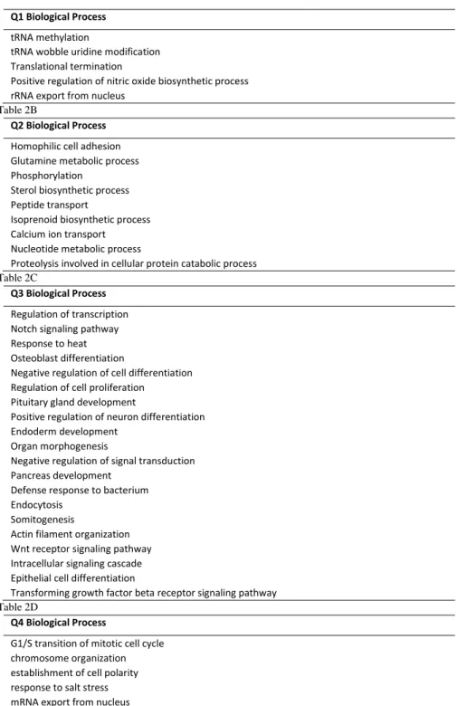
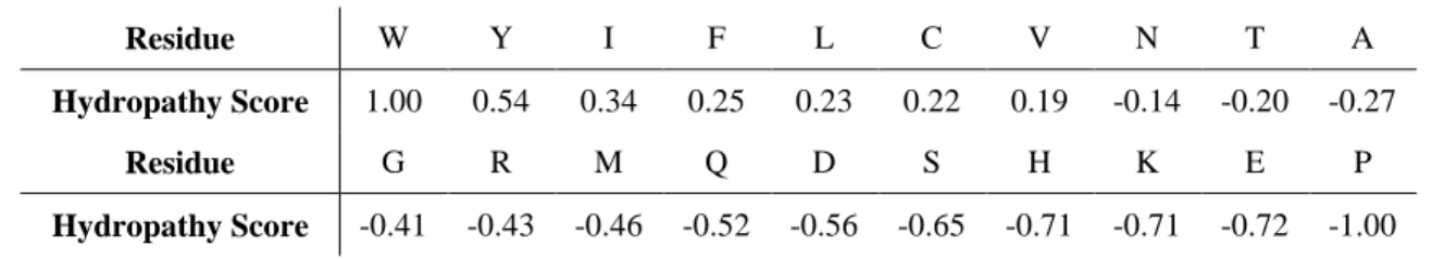
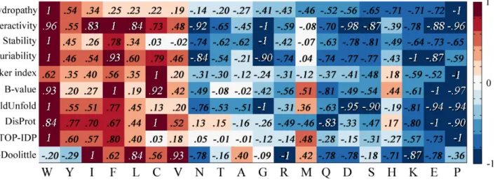
Table 2 lists those Biological Processes GO terms found to be distinctive for each quadrant. For Q1, four of the five distinctive GO terms deal with RNA. By the CH analysis, these proteins are highly charged, and this feature may be associated with RNA association. For the Q2 structured proteins (Table 2B), most of their GO terms are related to metabolic processes and transporters. These functions are typical for structured
proteins. For proteins in Q3, most of these GO terms are related to regulation or developmental pathways, including the Notch and Wnt pathways. As shown above, proteins in Q3 are likely to have both disordered and structured domains. Evidently these functions require both structured and disordered regions in the same proteins. Proteins in disorder quadrant (Q4 and table 1D) are mostly mitosis related.
Table 2 GO term analysis for four quadrants. Number of protein examples found for each GO term is listed on the right side.
Table 2A
Q1 Biological Process tRNA methylation
tRNA wobble uridine modification Translational termination
Positive regulation of nitric oxide biosynthetic process rRNA export from nucleus
Table 2B
Q2 Biological Process Homophilic cell adhesion Glutamine metabolic process Phosphorylation
Sterol biosynthetic process Peptide transport
Isoprenoid biosynthetic process Calcium ion transport Nucleotide metabolic process
Proteolysis involved in cellular protein catabolic process Table 2C
Q3 Biological Process Regulation of transcription Notch signaling pathway Response to heat Osteoblast differentiation
Negative regulation of cell differentiation Regulation of cell proliferation
Pituitary gland development
Positive regulation of neuron differentiation Endoderm development
Organ morphogenesis
Negative regulation of signal transduction Pancreas development
Defense response to bacterium Endocytosis
Somitogenesis
Actin filament organization Wnt receptor signaling pathway Intracellular signaling cascade Epithelial cell differentiation
Transforming growth factor beta receptor signaling pathway Table 2D
Q4 Biological Process
G1/S transition of mitotic cell cycle chromosome organization establishment of cell polarity response to salt stress mRNA export from nucleus
1.6 Discussion
Since ordered proteins have different types of substructures, it is reasonable to expect that IDPs may also have subtypes and that the different subtypes may have different functions. One previous study indicated that such disordered subtypes may exist157. However, the effort to subclassify IDPs such that each class has its own functional features still remains a difficult task.
Instead of relying on the training of existing data to build specific classifiers by common methods such as machine learning, we took an alternative approach. Different subtypes of IDPs should exhibit different biophysical features. Such features can be readily captured by applying two different prediction tools, CH and CDF, which use different biophysical characteristics for their calculations. We therefore developed a CH-CDF plot for IDP partition.
1.7 Structural Partitioning by the CH-CDF plot
Proteins partitioned by the CH-CDF plot show a very different PDB coverage rate. The structure quadrant (Q2) has many more proteins identified with at least one PDB protein than the disorder quadrant (Q4). The mixed quadrant (Q3) has a fraction of proteins with PDB hits almost comparable to those in the structure quadrant (Q2).
However, their coverage rate percentages are typically among 20%-30% range, while the ordered quadrant (Q2) are as high as 90%-100%. This suggests that mixed proteins (in Q3) have more ordered regions than those in the disorder quadrant (Q4).
Even though predicted to be structured, the proteins in the structure quadrant (Q2) have a significant fraction of examples with only 20% coverage (Figure 3, Q2). As indicated by the data in Table 1 and Figure 5, this result likely occurs because many mouse proteins have multiple structured domains. Thus, the entire protein is, overall, predicted to be structured by both the CH and CDF predictors, but if only one of the domains makes it into PDB, then such a protein could have a low coverage.
Some proteins in the mixed quadrant (Q3) and those in the disorder quadrant (Q4) have coverage percentage almost as high as 100%. After examining them individually, some of them are found to bind to ions, DNAs, RNAs, small molecules, etc. Such binding could potentially stabilize them, and lead to the formation of a crystal structure. However, there are indeed cases where they are monomers by themselves. We suspect that these proteins are close to the boundary of disorder and order, which we are in the process of testing.
One of our early hypotheses was that proteins with relatively low net charge and high hydropathy, e.g. predicted to be structured by CH, and yet predicted to be disordered by CDF, e.g. located in (Q3), might undergo hydrophobic collapse yet remain without stable structure. Such proteins would likely be native molten globules. An alternative hypothesis is that proteins in (Q3) simply contain mixtures of structured regions and disordered regions.
Our following experiments attempted to test the second hypothesis that (Q3) contains mostly proteins with both structured and disordered regions. We first showed that proteins in (Q3) have many more locally ordered sequence windows, indeed far more than the disordered quadrant (Q4), but less than the structure quadrant (Q2) (Table 1). We
then showed that the amino acid sequences in protein are predicted as mostly ordered if a PDB hit is identified for this region (Figure 5). When the sequence region is not matched with a PDB hit, it is most likely predicted to be disordered. So it seems that the quadrant (Q3) is likely to contain proteins containing relatively balanced contributions from
structured and disordered regions. For this reason here we have named the proteins in this quadrant mixed rather than collapsed disorder, which may have appeared in previous publications159,160. These observations don’t rule out the possibility that some of the proteins in (Q3) or even in (Q4) might be native molten globules. Further analysis and experiments are needed to identify such proteins and determine where they fall on the CH-CDF Plot.
1.8 The rare protein quadrant (Q1)
Proteins in this quadrant are predicted to be unstructured by CH plot, but ordered by CDF. The disordered prediction from CH plot implies that a protein has high charge and is hydrophilic. Thus, is should be rare for such a protein to be predicted to be structured by the CDF predictor; however, this is just what happens despite the high charge and hydrophilicity. So it is no wonder that the proteins in this quadrant are rare.
The density plot of PDB coverage percentage distribution for the proteins in (Q1) showed a similar pattern when compared to the structure quadrant (Q2) (Figure 3). The proteins in (Q1) also have many more proteins identified with a PDB hit than those in the disorder quadrant (Q4) (Figure 4). Therefore, one possibility is that these proteins are overall structured, with some high charged or hydrophilic residues, which is just the opposite of proteins in collapsed quadrant (Q3). The GO term analysis showed that 4 out
of 5 of the significant GO terms are related to nucleotide processing. Further analysis shows that many of the proteins in all four quadrants including (Q1) have net positive charges rather than net negative ones. We are in the process of determining whether the positively charged proteins in (Q1) are associated with RNA binding. One approach will be testing if this is the preferred quadrant for ribosomal proteins.
1.9 Disorder subtypes and IDP functions
We tested whether the protein compartmentalization by subtypes resulted in function partition as well. For this test, we did an analysis of GO terms to determine if some terms are biased relative to others in the various quadrants (see Methods for details).
Structured proteins exhibited significant biases towards enzymatic processes and transporters. Both of these processes are well known to be associated with structured proteins151–153.
Meanwhile, the disorder quadrant (Q4) is mainly biased towards GO terms with mitosis-related functions, which again agrees with previous observations151–153. On the other hand, the mixed quadrant (Q3) is highly involved in regulation pathways, which are important in development and differentiation. The recent publication on pluripotent stem cell-inducing proteins, which must be heavily involved in gene regulation, showed that these proteins are mostly localized in the mixed quadrant (Q3)160. The flexibility provided by disordered regions could be important in such signaling events. The
disordered regions could act as linkers connecting function domains. These regions could also directly bind to partners, functioning as Molecular Recognition Features (MoRFs). Such binding is usually accompanied by a disorder -> order transition. Because of their