How the ECB and the US fed set interest rates

HOHENHEIMER

DISKUSSIONSBEITRÄGE

How the ECB and the

US Fed Set Interest Rates

by

Ansgar Belke

and Thorsten Polleit

Nr. 269/2006

Institut für Volkswirtschaftslehre (520)

Universität Hohenheim, 70593 Stuttgart

Forthcoming in: Applied Economics* by

Ansgar Belke

_{Thorsten Polleit}

† _{University of Hohenheim, Stuttgart}

‡ _{Barclays Capital and HfB – Business School of Finance & Management, Frankfurt}

Abstract

Monetary policies of the ECB and US Fed can be characterised by “Taylor rules”, that is both central banks seem to be setting rates by taking into account the “output gap” and inflation. We also set up and tested Taylor rules which incorporate money growth and the euro-dollar exchange rate, thereby improving the “fit” between actual and Taylor rule based rates. In general, Taylor rules appear to be a much better way of describing Fed policy than ECB policy. Simulations suggest that the ECB’s short-term interest rates have been at a much lower level in the last two years compared with what a Taylor rule would suggest.

JEL code: E43, E58

Keywords: European Central Bank, Federal Reserve, Monetary policy, Taylor rule

Corresponding author: Prof. Dr. Ansgar Belke, University of Hohenheim, Department of Economics, Chair for International Economics (520E), 70593 Stuttgart, Germany, phone: ++49(0)711-459-3246, fax: ++49(0)711-459-3815, e-mail: [email protected]

I. Central bank reaction function: “Taylor rule”

The monetary policy strategy of the ECB is of particular interest for the analysis of business cycles but even more so for the ongoing debate on rules versus discretion in monetary policy.* In order to explain the interest rate decisions of the ECB, one may estimate Taylor rule (1993) type reaction functions, according to which an interest rate under the control of the ECB is made dependent on variables like the domestic inflation rate and the output gap.

In this contribution, we estimate several instrument policy reaction functions for the ECB in the period ranging from 1999 to 2005. The results might contribute to a better understanding of the bank’s interest rate setting behaviour. In particular, the result might help answering two questions, namely (i) whether the ECB has consistently followed a (stabilising) rule, and (ii) whether and how the ECB behaved differently than the US Fed Federal Reserve (Fed).

Due to the short history of EMU data, most papers on ECB monetary policy have up to now estimated a Bundesbank or a hypothetical ECB reaction function prior to 1999 and then, e.g. by testing its out-of-sample forecast properties, compared the implied interest rates with actual ECB rates.† There are only a few studies such as, for instance, Fourçans and Vranceanu (2002),

* _{See Carstensen and Colavecchio (2004). For the estimation of monetary policy}

reaction functions in general see, e.g., Huang and Lin (2006), Florio (2005) and Altavilla and Landolfo (2005). For an application to regime shifts in reaction functions see, for instance, Valente (2003).

†

See, e.g. Clausen and Hayo (2002), Faust et al. (2001), and Smant (2002) for the first approach and e.g. Clausen and Hayo (2002) and Gerlach-Kristen (2003) for the latter. For a good survey see Sauer and Sturm (2003).

Gerdesmeier and Roffia (2003), Ullrich (2003) and Surico (2003) which have actually estimated an ECB reaction function.

Most authors have so far chained up pre-EMU and post-EMU data to obtain long series. However, the implicit assumption of structural stability at the time of the EMU start inherent in these studies is hardly tenable according to our view. Moreover, it is questionable whether one can assume that the national central banks in the pre-EMU period followed on average a consistent strategy which can be compared without frictions with the strategy of the ECB (Belke and Gros, 2005). Hence, we base our analysis in this contribution purely on the euro area regime which started in January 1999.

The remainder of this paper proceeds as follows. In section II, we develop the theory of the Taylor rule and derive the empirical model. In section III, we compare official monetary policy with actual policy as measured by estimations of some variants of the Taylor rule. We present simulations for the ECB and the Fed and check for deviations of actual monetary policy from the central banks’ (Taylor) rules in section IV. Section V concludes.

II. Theory of the Taylor rule

In this section, we derive testable implications of the Taylor rule with a special focus on the ECB. Of course, analogous considerations apply to Taylor rules for characterising the Fed’s monetary policy.

We start from the usual baseline specification of the Taylor rule concept which looks as follows:

(1) it =ρ⋅it−1 +

(

) (

)

The variables included in this specification are the short-term interest rate it,

reflect the long-run weight of the variables output gap (y) and the inflation rate (π), respectively, while the parameter ρ describes the extent of interest rate smoothing chosen by monetary policy. Exactly following other studies in this field, the money market rate is used to approximate the relevant policy rate. As usual, we base our output gap and inflation rate variables on time series which are measured ex post for period t.

An important empirical question relates to the estimated weight on inflation, i.e. to the parameter β2. Since it is the real interest rate which actually drives

private decisions, the size of β2 needs to assure that – as a response to a rise in

inflation – the nominal interest rate is raised sufficiently to actually increase the real interest rate. This so-called ‘Taylor principle’ implies that the coefficient β2

has to be larger than 1 (Taylor, 1999b, and Clarida et al., 1998). If not, self-fulfilling bursts of inflation may be possible (see e.g., Bernanke and Woodford, 1997; Clarida et al., 1998; Clarida et al., 2000; Woodford, 2001). For monetary policy to have a stabilising impact on output, a less restrictive condition has to be fulfilled, i.e. β1 should be positive.

In practice, it is usually observed that, especially since the early 1990s, central banks worldwide tend to move policy interest rates in small steps without reversing their direction quickly (Amato and Laubach, 1999, Castelnuovo, 2003, and Rudebusch, 2002). To incorporate this pattern of interest rate smoothing, our equation (1) is viewed as the mechanism by which the target interest rate i* is determined. The actual interest rate partially adjusts to this target according to

(

)

= t

t i i

i ρ ρ , where ρ is the smoothing parameter. This results finally in

In addition to this baseline model, we consider either money growth or the nominal dollar-euro exchange rate as an additional argument contained in the ECB reaction function. The influence of the monetary pillar of the ECB monetary policy strategy is examined by the specification:

(2) i_t =ρ⋅i_t−1+

(

) (

)

which additionally includes the annual growth rate of money balances M3, mt. We include money growth to model the monetary pillar of the ECB strategy

which emphasizes the prominent role of M3 growth for interest rate decisions. This may reflect the leading indicator properties of money growth both for inflation (Altimari, 2001) and for the output gap (Coenen et al., 2001).

We also analyse whether ECB interest rate decisions are affected by changes in the nominal exchange rate of the dollar against the euro, exrt:

(3) i_t =ρ⋅i_t−1+

(

) (

)

According to its monetary policy strategy, the ECB claims to pay attention to a broad set of economic variables that may help to assess the presence of threats to price stability. We see two arguments which speak in favour of an inclusion of the exchange rate in the reaction function. First, while it is not clear whether central banks directly react and should react to exchange rate changes (Taylor, 2001), the ECB might have been particularly tempted to counteract devaluations in the first years of EMU in order to establish the notion of a strong euro as an equivalent successor of the deutschmark. Second, a direct influence of exchange rate changes in the instrument rule can pay off in terms of reduced inflation variance (Ball, 1999, Taylor, 1999b).

III. Empirical Evidence of the Taylor rule 1. Preliminaries

Many studies show that monetary policy in Germany‡ and the hypothetical euro area prior to 1999 followed the Taylor principle with β2 exceeding 1.§ With

respect to ECB policy, however, the preliminary consensus reached looks rather different. The results gained by Gerdesmeier and Roffia (2003) and Ullrich (2003) who use standard output gap measures based on Hodrick-Prescott-filtered industrial production contradict those brought forward both by Fourçans and Vranceanu (2002) who take the annual growth rate of industrial production as a measure of the business cycle and by the literature on Taylor rules for both Germany and the hypothetical euro area. While Fourçans and Vranceanu (2002) find the ECB to react strongly to variations in the inflation rate and much less to output variations, both Gerdesmeier and Roffia (2003) and Ullrich (2003) somewhat surprisingly identify small reactions to inflation and - both in relative and in absolute terms - strong responses to output deviations. Fourçans and Vranceanu (2002) arrive at coefficient estimates of β1=0.18 and β2=1.16 for the

sample 1999:4-2002:2. Gerdesmeier and Roffia (2003) estimate β1=0.30 and

β2=0.45 based on a sample 1999:1-2002:1. For a sample of 1999:1-2002:8,

‡ _{See, for instance, Clarida et al. (1998), Clausen and Hayo (2002), Faust et al. (2001),}

Peersman and Smets (1998) and Smant (2002).

§

See, e.g., Clausen, Hayo (2002), Gerlach-Kristen (2003), Gerlach, Schnabel (2000), Peersman, Smets (1998), and Ullrich (2003).

Ullrich (2003) comes up with β1=0.63 and β2=0.25.** Furthermore, Ullrich (2003)

observes a structural break between pre-1999 and post-1999 monetary policy in the euro area.

2. The data issue

Following most of the literature, we use ex-post realized data and apply the generalized method of moments (GMM) to estimate the ECB and the Fed reaction function. In order to compare a Taylor Rule with actual monetary policy, we need to find proxies for the stance of monetary policy, inflation and the output gap. We conduct the GMM estimations both for quarterly and monthly data. All data are seasonally adjusted. Data are taken from Bloomberg and Thomson Financial.

The sample period for our estimations of the ECB and Fed interest setting behaviour is 1999Q1 to 2005Q02. We measure actual monetary policy by the three-month money market rates (ISR_EU and ISR_US). Euro area inflation is measured by the year-on-year percentage change in the harmonised index of consumer prices for the euro area (D4LNCPI_EU). US inflation is calculated on the basis of the consumer price index (D4LNCPI_US). Money growth is measured by the year-on-year percentage change in M3 for the euro area (D4LNM3_EU), and by the year-on-year percentage change in M2 for the US (D4LNM2_US). The output gap (OUTPUTGAP_EU and OUTPUTGAP_US) is calculated by the first difference between real GDP in logs and the

** _{A further example is Surico (2003a) who comes up with the following estimates:}

Prescott filtered log real GDP with the smoothing parameter set at λ = 1600).†† As exchange rate variable we used the annual growth rate of the nominal dollar exchange rate vis-à-vis the euro (GROWTH_EUROUSD), i.e. the first difference of order 4 of the log exchange rate (Taylor, 2001, p. 6). Since the null hypothesis of non-stationarity cannot be rejected for the levels of our exchange rate variable but can be rejected for the first differences at the usual 5 percent level, we used first differences of the exchange rate variable in our regressions.‡‡ As usual, we applied the first difference of order 4 in strict analogy with our measure of the inflation rate. An increase of the exchange rate variable indicates an appreciation of the euro.

As far as the output gap specification is concerned, we strictly follow Clarida

et al. (1998) and Faust et al. (2001) and finalize our analysis with the complementary use of monthly data. In this case of monthly data, we use the industrial production index for the euro area and apply a standard Hodrick-Prescott filter (with the smoothing parameter set at λ = 14,400) to calculate the

†† _{However, in the simulations part of this paper, we complementarily use monthly data}

(Belke and Gros, 2005). Since our measure of the output gap based on industrial production is much more volatile than Taylor’s (1993) original GDP-based output gap, the results might be biased and we mainly focus on the results based on GDP series and quarterly data, as is also sometimes preferred in the literature (see, e.g. the survey by Ullrich, 2003).

‡‡

We used a wide spectrum of unit root tests, among others, e.g., the ADF-test, the Elliott-Rothenberg-Stock DF-GLS test and the Kwiatkowski-Phillips-Schmidt-Shin test. The results are available on request.

output gap as the deviation of the logarithm of actual industrial production from its trend.§§

In the case of monthly data, we base our analysis of the ECB behaviour on the period from January 1999 to August 2005. The analysed time period for the US comprises the “Greenspan era”, starting in August 1987. As exchange rate variable we used the annual growth rate of the nominal dollar exchange rate vis-à-vis the euro (GROWTH_USEUR), i.e. the first difference of order 12 of the log exchange rate. An increase of the exchange rate variable indicates an appreciation of the euro.

3. The estimation issue

The GMM approach essentially consists of an instrumental variables estimation of equation (1) and becomes necessary because at the time of an interest rate decision, the ECB cannot observe the ex post realized contemporaneous right-hand side variables in equations (1) to (3). Hence, it bases its decisions on information which comprises lagged variables only. The weighting matrix in the objective function is chosen in order to allow the GMM estimates to be robust to possible heteroskedasticity and serial correlation of unknown form in the error terms (for a recent application see Carstensen and Colavecchio, 2004).

The chosen instruments need to be predetermined at the time of an interest rate decision. Hence, they have to be dated on period t-1 or earlier. They should help to predict the contemporaneous variables which are still unobserved at time t.

§§

Despite the increasing share of services in the overall economy, it is still commonly assumed that the industrial sector is the ‘cycle maker’ and that it leads significant parts of the economy. See Sauer and Sturm (2003).

For exactly this purpose, we include the first four lags of the nominal interest rate, inflation, the output gap, money growth, and the euro-dollar exchange rate. The former three variables are typically used as instruments in related work (Sauer and Sturm, 2003, Gerdesmeier and Roffia, 2003, and Ullrich, 2003). We also include money growth and the nominal euro-dollar exchange rate. The choice of a relatively small number of lags for the instruments is intended to minimize the potential small sample bias that may arise when too many over-identifying restrictions are imposed. To confirm that we have chosen an appropriate instrument set, we run a first stage regression of inflation and other variables of equation (1) to (3) on the instrumental variables and perform an F-test for their joint significance (Kamps and Pierdzioch, 2002).

A second important property of the instrumental variables is their exogeneity with respect to the central bank decisions and, hence, their uncorrelatedness with the disturbances which reflect deviations from the policy rule that are unpredictable ex ante. To test this property, we perform a standard J-test for the validity of the over-identifying restrictions (Hansen, 1982, and Tables 1 and 2). We dispense with the robustness checks by means of the ordinary OLS procedure which are widely used in the literature because otherwise the regressors would unlikely be weakly exogenous.

4. Empirical results for ECB policy

Table 1 presents a review of three different Taylor rule estimations based on our equations (1) to (3), using quarterly data. Column (3, equation (1)) shows the baseline scenario of equation (1). The degree of interest rate smoothing and the ECB’s response to inflation is rather small, whereas the weight of the output gap is large (and significantly larger than for inflation).

Compared to the original Taylor rule which postulates weights of 0.5 both for the output gap and inflation, respectively, the influence of the business cycle situation on the decisions of the ECB seems to be strong. However, the inflation weight proves to be smaller than according to the original Taylor rule and falls considerably below 1. Hence, the so-called Taylor principle β2>1 which would

guarantee that an increase in the nominal interest rate causes an increase in the real interest rate with the desired dampening impact on inflation is clearly not fulfilled. However, note that our findings are in line with the few other available studies.

- Table 1 here -

Adding money growth and the exchange rate change to the Taylor rule specification (column 4, equation (2)), leads to a slightly different picture. Independent from the significance of the output gap and the inflation rate, we are able to establish a significant impact of money on the interest rate decisions. Moreover, the coefficient of money growth is positive as expected from theory. Presumably, this result is caused by the fact that the ECB considered the high money growth rates in the aftermath of the stock market downswing as portfolio adjustments that did make interest rate responses necessary.*** At the same time and most remarkably, the coefficient of inflation changes becomes negative. One explanation for this quite striking result might be that the ECB pursued its

***

For a detailed analysis of the effects of the stock market downswing and the accompanying financial uncertainty on EMU money demand and on measures of excess liquidity derived from money demand, see Carstensen (2003) and Greiber and Lemke (2005).

inflationary course by means of reacting to higher money growth rather than to actual inflation.

Another explanation might be that the ECB might not have responded strongly to actual inflation due to uncertainty and data release lags. Since inflation expectations on the part of the ECB (operationalised by the bank’s near-term inflation outlook as published in the Bulletins) tended to fall short of actual future inflation in our sample, it should make a difference for the estimates which variables are used – actual or expected ones.††† Finally, the time profile of the lag structure in the relation between money growth and consumer price inflation works reasonably well as an explanation – as shown by an additional investigation of the correlations between the respective time series. Although both parameters for inflation and for money growth appear to be very close, a simple Wald test of coefficient restrictions (whose results are available on request) reveals that the sum between both coefficient estimates is significant, i.e. we have to reject the null hypothesis that the estimates are numerically the same in absolute values. Hence, there is no need to look for a special explanation of numerically equal parameter estimates.

†††

Giannone, Reichlin and Sala (2002), p. 11, deliver a third competing argument. They argue that the reaction function used here is not conditioned on shocks like demand or technology shocks but on the variables themselves. The use of a reaction function not conditioned on shocks might result in a coefficient smaller than unity depending on the ratio of inflation variance caused by demand to inflation variance caused by technology. A low value of this ratio causes a small coefficient. For a similar argument see also Ullrich (2003), p. 10.

In our final specification (column (5), equation (3)), the inflation variable even becomes insignificant. However, the coefficient of the output gap, albeit smaller, stays highly significant. Again, also in specification 3 the high significance and the high value of the estimated coefficient of the output gap in the ECB reaction function deserves special attention, even though it possesses a coefficient lower than the other tabulated specifications. Thus, there is again clear evidence of a business cycle orientation of the ECB.

Even though the coefficient of the exchange rate is relatively small compared to the ones of the other explanatory variables, it is highly significant and displays the expected negative sign. As discussed in Taylor (2001), an appreciation of the euro leads to a relaxation of monetary policy. Moreover, our point estimates are in the range analysed by Taylor (1999b). According to our estimates, a one percent devaluation of the euro leads to a long-run interest increase of four basis points. The significance of the coefficient of the exchange rate – although it is quite small – suggests that including the exchange rate leads to a stable specification (3) which describes the monetary policy rule of the ECB pretty well. By this, we empirically corroborate the rule of thumb that – as a monetary policy rule - a substantial appreciation of the exchange rate furnishes a prima facie case for relaxing monetary policy (Obstfeld and Rogoff, 1995, pp. 93, and section II).

One interpretation of this rule of thumb would be that the coefficient of the exchange rate change is less than zero. Then a higher than normal exchange rate would call on the central bank to lower the short-term interest rate, which presumably would represent a relaxing of monetary policy. Or, the appreciation of the exchange rate today (period t, say) will increase the probability that the central bank will lower the interest rate in the future (period t+1, say). With a rational expectations model of the term structure of interest rates, these expectations of

lower future short term interest rates will tend to lower long-term interest rates today. Thus the appreciation of the exchange rate, through the effects of exchange rate transmission and the existence of a policy rule, will result in a decline in interest rates today. However, our results do not support the competing view that policy makers should heed the Obstfeld-Rogoff warning that substantial departures from PPP, in the short run and even over decades make such a policy reaction to the exchange rate undesirable.

Let us finally turn to the issue of interest rate smoothing. Note that our estimates of ρ, which range from 0.65 to 0.75, are quite high. However, coefficients are not so close to 1 so that the estimation uncertainty of the long-run weights would become really large. In fact, our results are in line with Gerdesmeier and Roffia (2003) who estimate ρ to be 0.72 and Fourçans and Vranceanu (2002) who arrive at an estimate of ρ=0.73.

The findings above appear to be robust in the sense that the J-statistic testing the over-identifying restrictions is insignificant across all specifications tested. In Table 1, we use the J-statistic to test the validity of over-identifying restrictions when we have (as in our case) more instruments than parameters to estimate. Under the null-hypothesis, that is the over-identifying restrictions are satisfied, the J-statistic multiplied by the number of regression observations is asymptotically distributed with degrees of freedom equal to the number of over-identifying restrictions (Favero, 2001). According to the results tabulated in the second last row of Table 1, all our models are correctly specified because all p-values are higher than their critical counterparts.

Overall, the results displayed in Table 1 are conclusive. All regressions show that interest rate policy from 1999 on did not follow the Taylor principle as β2

does not exceed 1 consistently. The inflation parameter for the ECB period (β2) is

usually lower than the output parameter (β1) and does not exceed one. Hence,

from this pattern one might even conclude that the ECB tended to accommodate changes in inflation. This is also suggested by the standard specification in column 3 of Table 1 which reports a positive and significant coefficient for inflation.

The results presented above accentuate those of Gerdesmeier and Roffia (2003) and Ullrich (2003), who suggest that the ECB reacts to a rise in expected inflation by raising nominal short-term interest rates by a relatively small amount and thus letting real short-term interest rates decline. Hence, instead of continuing the Bundesbank’s inflation stabilising policy, the ECB appears to have followed a policy rather comparable to the pre-Volcker era of the Fed, for which e.g. Taylor (1999a) and Clarida et al. (2000) have found values for β2 well below one.‡‡‡

5. Estimation results for Fed policy

Table 2 presents a review of three different Taylor rule estimations based on equations (1) to (3) for the US, again using quarterly data.

The results for the basic specification are displayed in Table 2 (column (3), equation (1)). Using ex post measured variables in the baseline specification (1) leads to a rather strong interest rate smoothing, a large weight of the output gap and an even larger one of inflation. Compared to the original Taylor rule with weights of 0.5 both for the output gap and inflation, respectively, the impact of

‡‡‡ _{Taylor (1999a) arrives at values of β1 = 0.25 and β2 = 0.81 with ex-post data for}

the US for that period, while Orphanides (2001) estimates a forward-looking rule with real-time data and reports β1= 0.57 and β2 =1.64.

inflation on Fed decisions is relatively strong. However, the weights of inflation and of the output gap are not too different. The inflation weight is larger than in the original Taylor rule and considerably above 1. Hence, the so-called Taylor principle β2>1 is clearly fulfilled. Hence, an increase in the nominal interest rate

tends to cause an increase in the real interest rate and a dampening of inflation.

- Table 2 here -

Adding money growth to the baseline variables yields (column (4), equation (2)), which has a stronger degree of interest rate smoothing than before. This does not change the pattern of the results for inflation and the output gap at all. However, in contrast to our estimates for the ECB, the sign of the coefficient of M2 growth is negative. Hence, higher M2 growth tends to lead to lower realisations of the policy variable.

If we finally include dollar-euro exchange rate changes in our Taylor rule specification (column (5) of Table 2), the coefficient of inflation remains highly significant. The coefficient of the output gap is even larger and again highly significant. Even though the coefficient of the exchange rate is relatively small compared to the ones of the other explanatory variables, it is clearly significant and has the expected positive sign (see section II). An appreciation of the euro (a rising exchange rate) leads to a more restrictive monetary policy of the Fed. According to our estimates, a one percent devaluation of the dollar leads to a long-run interest increase of twelve basis points. This interest rate reaction is three times as high as in the ECB case.

At last, we should make some comments on the estimated extent of the Fed’s interest rate smoothing behaviour (row 2 of Table 2). The parameter ρ is estimated to be significantly larger than in the euro area and falls into a range between 0.84 and 0.91. From an economic point of view, our evidence on interest

rate smoothing can be interpreted as follows. Since it captures the impact of the lagged interest rate on the current interest rate decision i becomes more and more important as ρ tends to one. Consequently, the relative importance of other explanatory variables should diminish. It may even be the case that they are not suitable anymore to explain the long run patterns of the policy variable (see, e.g., Carstensen and Colavecchio, 2004, p. 11). However, we observe exactly the opposite in the case of the Fed. The additional variables are highly significant and have coefficients which are large in absolute and relative terms. Overall, the smoothing parameter estimates a bit more away from 1 are obtained in the specifications 1 and 3 where the money growth indicator is not included.

IV.

Simulations

To shed light on the question as to whether the central bank complied with the Taylor rule in the more recent past, we make use of one-period-ahead forecasts. By doing so, we should be able to quantify the difference between the actual and the fitted, or Taylor, interest rate. We make use of static one-step-ahead forecasts based on our specifications of the Taylor reaction functions including interest smoothing behaviour.

In this context, (a) in-sample and (b) out-of-sample forecasts will be produced. Case (a) allows to investigate whether the central bank sets interests rates according to a Taylor rule which is estimated based on data for the whole available sample period. Case (b) shall provide insights as to whether the central banks stuck to their rule, which was estimated for a sub-period, throughout the total period under review.

While our in-sample forecasts (case (a)) are based on exactly the same estimations and especially the same estimation period which were presented in

Tables 1 and 2, our out-of-sample forecasts (case (b)) necessitate the re-estimation of the same specifications for a shorter time-horizon. This ex-ante forecasting or post-sample prediction exercise helps forecasting observations that do not appear in the data set used to estimate the forecasting equation. Since case (b) would have resulted in a serious lack of degrees of freedom due to insufficient data points, we decided to make use of monthly data if we enact out-of-sample forecasts.§§§

Figures 1 and 2 illustrate the results of the in-sample forecasts of monetary policy according to a Taylor rule which is estimated over the whole available sample independent on the start of the forecast period (case (a)). Figures 3 and 4 exhibit the prediction of a Taylor rule over the whole sample when this Taylor rule is estimated only up to the start of the out-of-sample forecast period (case (b)). Each Figure contains three graphs which depict the course of actual monetary policy together with the Taylor rule estimated by equations (1) to (3).

Our first choice for setting the start date of the forecast period is (the 11th) September 2001, because this started a period of unprecedented political and financial market instability. The second choice would be the turn-of-year 2000/01, with which came the meltdown of stock market valuations (Belke and Gros, 2005). The exact dates of the chosen sample splits are recorded in the tables.

- Figure 1, 2, 3 and 4 here -

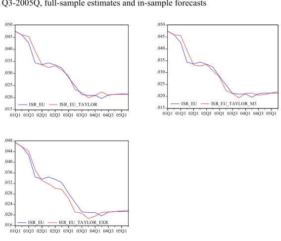
As far as the in-sample forecasts for the euro area are concerned, the estimated realisations of the central bank rate follow closely the actual interest

§§§

Inoue and Kilian (2002) show that in-sample tests of predictability are at least as credible as the results of out-of-sample tests. Hence, there is no reason to emphasize only one type of forecasts a priori.

rate. This should be of little surprise, given the rather high R-squared of the estimations in Tables 1 and 2. In the most recent quarters in 2005, however, the Taylor rate slightly exceeded the actual ECB rate (the opposite is the case for the first two quarters of 2005 with regard to the Fed). This would imply that euro interest rates are currently slightly too low as compared with the implicit Taylor rule.

Next, according to the Taylor specifications including money growth, both monetary policies have been too expansionary during the third and the fourth quarter of 2001 and the first and the second quarter of 2004. A similar pattern emerges for specifications (2) and (3). In contrast, if one considers the specification including the exchange rate, euro area monetary policy appeared to have slightly too strict from the first quarter of 2002 until the first quarter of 2004. Let us now turn to our out-of-sample forecasts of the policy variable for the ECB and the Fed.

Note again that out-of-sample forecasting represents a particularly interesting exercise, as it allows detecting deviations of actual monetary policy rates from normative Taylor rate levels. Since it is generally agreed that evaluating forecasts must be done exclusively on their ex ante performance, we mainly comment on Figures 3 and 4.

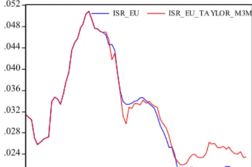
As far as the euro area is concerned, one finds a significant negative deviation of the actual interest rate from the estimated interest rate which corresponds to the (Taylor) rule from the midst-of-2003 on up to August 2005. This is striking especially because we also included the estimated extent of interest rate smoothing in the normative Taylor interest rate and, by this, corrected for stickiness in interest rate setting in times of uncertainty. Overall, we conclude that ECB monetary policy has been to be too expansionary already since two

years. The negative deviations of actual rates from the rule might be interpreted as a clear sign that the bank has significantly downgraded the role of money in its policy strategy and actual policy making since May 2003.

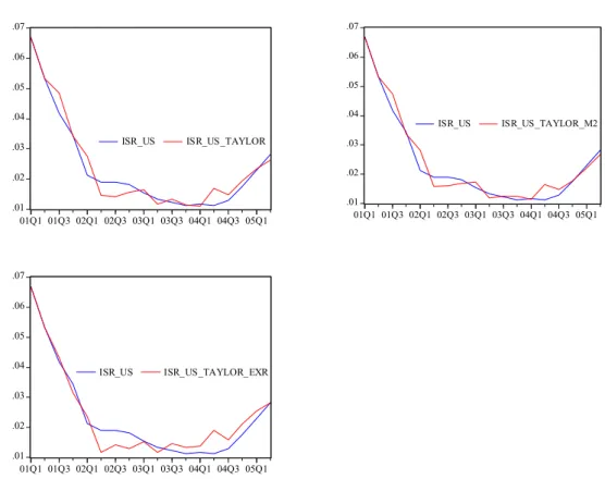
Fed actions appear to have been significantly different from that of the ECB. In fact, the Fed seems to have strictly followed its Taylor rule since 2000/01. Such a conclusion alters only if the change of the euro-dollar exchange rate is included in the Taylor rule specification. Here, the Fed did not react to the depreciation of the dollar as sharply as it did prior to 2000/2001. One explanation for this pattern might be that, given its multi-indicator approach, the Fed might have tried to help reducing the current account deficit by short-term rate changes. This could also explain why the fit between the actual and Taylor rate as shown in Figure 4, third graph, is not as perfect as depicted in Taylor (1993).

In general, the standard Taylor rule, with the Taylor’s normative weights, appears to be a much better way to characterise the rate setting behaviour of the Fed than that of the ECB. Moreover, the Fed has shown a stronger (preference for) interest rate smoothing under the Taylor rule compared with the ECB. That might explain why, following the crisis of 2000/2001, the Fed’s rates have remained in line with the Taylor rate whereas the ECB has deviated from its pre-crisis Taylor rule policy behaviour.

V. Concluding Remarks

According to the findings presented in this paper, the interest rate setting behaviour of the ECB and the Fed in the period 1999 to 2005 and 1987 to 2005, respectively, can be pretty well characterised by some form of Taylor rule.

However, the standard Taylor rule appears to be a much better tool for modelling the behaviour of the Fed than that of the ECB.****

The empirical estimates for the euro area suggest that the ECB put a larger weight on the output gap relative to inflation. Such a conclusion is shared by other authors. Faust et al. (2001) argue that the ECB puts too high a weight on the output gap relative to inflation, especially in comparison to the Bundesbank. However, the low weight which the ECB has assigned to inflation might be due to the fact that inflation was fairly low in the sample period. Moreover, the estimates also show that money growth appear to have played an important role in the ECB’ rate setting. Moreover, the exchange rate had a small, albeit significant effect as well.

The test results indicate that the Fed has been following the estimated Taylor rule in a rather stable manner during the Greenspan era. This does not change if money growth is included as an additional variable in the Taylor rule, but it becomes somewhat less obvious when the change of the euro-dollar exchange rate is taken into account. As a particularly interesting side-aspect, money growth seems to have played an important role in Fed rate decisions as well.

Comparing the Taylor rule estimations of the two central banks, Fed displayed a much greater tendency for interest rate smoothing compared with its counterpart in the euro area. This might explain why, following the crisis of 2000/2001, the Fed’s rates have remained fairly in line with the Taylor rate (even

****

See, however, Österholm (2005) who conjectures that the Taylor rule appears to be a questionable tool for evaluation of the Federal Reserve during the investigated samples.

in view of a series of unprecedented interest rate cuts), whereas the ECB has deviated from its pre-crisis Taylor rule policy behaviour.

In fact, the findings do not suggest that the ECB has followed a stable rate setting pattern stabilizing throughout the sample period, whereas the Fed appears to have adhered to its rate setting behaviour. In fact, the ECB seems to have pursued too expansionary a policy after 2000/01.

Looking at contemporaneous Taylor rules, our results suggests that the ECB has de facto even accommodated changes in inflation and, hence, might have even followed a pro-cyclical, e.g. destabilising, policy. In contrast to the Fed, the ECB’s nominal policy rate changes were not large enough to actually influence real short term interest rates. Such an interpretation gives rise to the conjecture that the ECB follows a policy quite similar to the pre-Volcker era of US monetary policy, a time also known as the “Great Inflation” (Taylor, 1999a).

However, in view of the results above some words of caution might be in order. In general and in relation to data used in the applications, the number of the observations is rather small (only 26 - 1999Q1 to 2005Q2). Therefore, the estimations risk to be not robust. It is important to recognize this drawback in the analysis. We addressed this caveat in the paper for instance when we enhanced the frequency of the data set, i.e. applied monthly instead of quarterly data.

However, one should always be aware of the fact that time series properties are more a question of the time span (sample issue) than of the numbers of observations investigated. Hence, we will be able to come up with more satisfactory results in terms of degrees of freedom only when some further time will have elapsed. Nevertheless, it is time now to follow pioneers in the field (see section III.1) and to actually estimate an ECB reaction function. We feel all the more legitimised to do so because (a) our time span clearly goes beyond those

samples used in the above mentioned studies by nearly 100 percent and (b) we follow those studies by complementarily using monthly data in order to escape the problem of limited degrees of freedom (although one should be aware that this is only a limited device to assess time series properties more accurately).

More specifically, Clarida et al. (2000, p. 154) argues that a short sample with little variability in inflation, especially with only small deviations from the target rate, might lead to too low an estimate of the inflation parameter. So far, data are only available for less than two completed business cycles and the actual inflation rate is close to the target the ECB has set itself. In that sense, recent inflation rates are not at all comparable to those during the 1970s. It might also be the case that the ECB would act much more aggressively against larger deviations of inflation from its own goal than can be seen in the data so far. As suggested by e.g. Clarida and Gertler (1996), central banks react differently to expected inflation above trend as compared to expected inflation below trend. They show that the Bundesbank clearly reacted in the former case, whereas in the latter case they hardly responded. Given data limitations, it is too early for us to tell whether or not the same holds for the ECB.

References

Altavilla, C. and Landolfo, L. (2005) Do Central Banks Act Asymmetrically? Empirical Evidence from the ECB and the Bank of England, Applied Economics, 37, 507-519.

Altimari, S. N. (2001) Does Money Lead Inflation in the Euro Area?, ECB Working Paper, 63, European Central Bank, Frankfurt/Main.

Amato, J. D. and T. Laubach (1999) The Value of Interest-rate Smoothing: How the private sector helps the Federal Reserve, Federal Reserve Bank of Kansas City Economic Review, 84 (3), 47-64.

Ball, L. (1999) Policy Rules for Open Economies, in Monetary Policy Rules (Ed.) J. B. Taylor, University Press, Chicago, 127-144.

Belke, A. and Gros, D. (2005) Asymmetries in Transatlantic Monetary Policy-making: Does the ECB Follow the Fed?, forthcoming in Journal of Common Market Studies, 43 (5), December.

Bernanke, B. and Woodford M. (1997) Inflation Forecasts and Monetary Policy,

Journal of Money, Credit, and Banking, 24, 653-684.

Carstensen, K. (2003) Estimating the ECB Policy Reaction Function, forthcoming in German Economic Review.

Carstensen, K., and Colavecchio R. (2004) Did the Revision of the ECB Monetary Policy Strategy Affect the Reaction Function?, Kiel Working Papers, 1221, Kiel Institute for World Economics, Kiel.

Castelnuovo, E. (2003) Describing the Fed’s Conduct with Taylor Rules: Is Interest Rate Smoothing Important?, ECB Working Paper, 232, European Central Bank, Frankfurt/Main.

Clarida, R. and Gertler, M. (1996) How the Bundesbank Conducts Monetary Policy, NBER Working Paper, 5581, NBER, Cambridge, MA.

Clarida, R., Galí, J. and Gertler M. (1998) Monetary Policy Rules in Practise: Some International Evidence, European Economic Review, 42, 1033-1067. Clarida, R., Galí, J. and Gertler M. (1999) The Science of Monetary Policy: a

New Keynesian Perspective, Journal of Economic Literature, 37 (4), 1661-1707.

Clarida, R., Galí, J. and Gertler M. (2000) Monetary Policy Rules and Macroeconomic Stability: Evidence and Some Theory, Quarterly Journal of Economics, 115, 147-180.

Clausen, V. and Hayo B. (2002) Monetary Policy in the Euro Area – Lessons from the First Years, ZEI Working Paper, B 02-09.

Coenen, G., Levin A. and Wieland V. (2001) Data Uncertainty and the Role of Money as an Information Variable for Monetary Policy, ECB Working Paper,

84, European Central Bank, Frankfurt/Main.

Faust, J., Rogers, J. H. and Wright J. H. (2001) An Empirical Comparison of Bundesbank and ECB Monetary Policy Rules, International Finance Discussion Papers, 705, Board of Governors of the Federal Reserve System. Favero, C. (2001) Applied Macroeconometrics, Oxford University Press, Oxford. Favero, C., Freixas, X., Persson, T. and Wyplosz, C. (2000) One Money, Many

Countries. Monitoring the European Central Bank 2, Center for Economic Policy Research, London.

Florio, A. (2005) Asymmetric Monetary Policy – Empirical Evidence for Italy,

Applied Economics, 37, 751-764.

Fourçans, A. and Vranceanu, R. (2002) ECB Monetary Policy Rule: Some Theory and Empirical Evidence, ESSEC Working Paper, 02008, forthcoming in

European Journal of Political Economy.

Gali, J. (2002) Monetary Policy in the Early Years of EMU, In EMU and Economic Policy in Europe: the Challenges of the Early Years (Eds.) M. Buti and A. Sapir, Edward Elgar, Cheltenham.

Gerdesmeier, D. and Roffia, B. (2003) Empirical Estimates of Reaction Functions for the Euro Area, ECBWorking Paper, 206, European Central Bank, Frankfurt am Main.

Gerlach, S. and Schnabel, G. (2000) The Taylor Rule and Interest Rates in the EMU Area, Economics Letters, 67, 165-171.

Gerlach-Kristen, P. (2003) Interest Rate Reaction Function and the Taylor Rule in the Euro Area, ECB Working Paper, 258, European Central Bank, Frankfurt am Main.

Giannone, D., Reichlin, L. and Sala, L. (2002), Tracking Greenspan: Systematic and Unsystematic Monetary Policy Revisited, CEPR Discussion Paper, 3550, London.

Greiber, C. and Lemke W. (2005) Money Demand and Macroeconomic Uncertainty, Bundesbank Discussion Paper, Economic Studies, 26/2005, Frankfurt am Main.

Hansen, L. P. (1982) Large Sample Properties of Generalized Method of Moments Estimators, Econometrica, 50, 1029-1054.

Huang, H.-C. and Lin, S.-C. (2006) Time-varying Discrete Monetary Policy Reaction Functions, Applied Economics, 38, 449-464.

Inoue, A. and Kilian, L. (2002) In-sample or Out-of-sample Tests of Predictability: Which One Should We Use?, ECB Working Paper, 195, European Central Bank, Frankfurt/Main.

Kamps, C. and Pierdzioch C. (2002) Geldpolitik und vorausschauende Taylor-Regeln – Theorie und Empirie am Beispiel der Deutschen Bundesbank,

Kieler Arbeitspapiere, 1089, Institut für Weltwirtschaft, Kiel.

Obstfeld, M. and Rogoff, R. (1995) The Mirage of Fixed Exchange Rates, Journal of Economic Perspectives, 9, 73-96.

Österholm, P. (2005) The Taylor Rule and Real-time Data – a Critical Appraisal,

Orphanides, A. (2001) Monetary Policy Rules, Macroeconomic Stability and Inflation: A View from the Trenches, Federal Reserve Board, Finance and Economics Discussion Series, 2001-62.

Peersman G. and Smets, F. (1998) Uncertainty and the Taylor Rule in a Simple Model of the Euro-area Economy, Ghent University Working Paper.

Rudebusch, G. D. (2002) Term Structure Evidence on Interest-rate Smoothing and Monetary Policy Inertia, Journal of Monetary Economics, 49, 1161-1187. Sauer, S. and Sturm, J.-E. (2003) Using Taylor Rules to Understand ECB

Monetary Policy, CESifo Working Paper, 1110, Center for Economic Studies, University of Munich.

Smant, D. J. C. (2002) Has the European Central Bank Followed a Bundesbank Policy? Evidence from the Early Years, Kredit und Kapital, 35 (3), 327-43. Surico, P. (2003) How Does the ECB Target Inflation?, ECB Working Paper, 229,

European Central Bank, Frankfurt am Main.

Surico, P. (2003a) Asymmetric Reaction Functions for the Euro Area, Oxford Review of Economic Policy, 19 (1), 44-57.

Taylor, J. B. (1993) Discretion versus Policy Rules in Practice, Carnegie-Rochester Conference Series on Public Policy, 39, 195-214.

Taylor, J. B. (1999a) A Historical Analysis of Monetary Policy Rules, in

Monetary Policy Rules, (Ed.) J. B. Taylor, University of Chicago, Chicago. Taylor, J. B. (1999b) The Robustness and Efficiency of Monetary Policy Rules as

Guidelines for Interest Rate Setting by the European Central Bank, Journal of Monetary Economics, 43, 655-679.

Taylor, J. B. (2001) The Role of the Exchange Rate in Monetary Policy Rules,

Ullrich, K. (2003) A Comparison Between the Fed and the ECB: Taylor Rules,

ZEW Discussion Paper, 03-19, Mannheim.

Valente, G. (2003) Monetary Policy Rules and Regime Shifts, Applied Financial Economics, 13, 525-535.

Woodford, M. (2001) The Taylor Rule and Optimal Monetary Policy, American Economic Review, 91, 232-237.

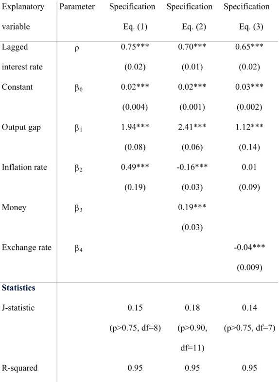
Table 1: Empirical Taylor reaction functions of the ECB GMM estimations, Quarterly data, 1999Q1-2005Q2 Explanatory variable Parameter Specification Eq. (1) Specification Eq. (2) Specification Eq. (3) Lagged interest rate ρ 0.75*** (0.02) 0.70*** (0.01) 0.65*** (0.02) Constant β0 0.02*** (0.004) 0.02*** (0.001) 0.03*** (0.002) Output gap β1 1.94*** (0.08) 2.41*** (0.06) 1.12*** (0.14) Inflation rate β2 0.49*** (0.19) -0.16*** (0.03) 0.01 (0.09) Money β3 0.19*** (0.03) Exchange rate β4 -0.04*** (0.009) Statistics J-statistic 0.15 (p>0.75, df=8) 0.18 (p>0.90, df=11) 0.14 (p>0.75, df=7) R-squared 0.95 0.95 0.95

Notes: Standard errors are given in parentheses below the estimated values (*/**/*** indicating significance on the 10/5/1 percent level), p-values are given in parentheses below the J-test statistics (df = degrees of freedom). For the GMM estimation the first four lags of the short-term interest rate, the inflation rate, the output gap, the money growth rate (if implemented), and the rate of change of the dollar-euro exchange rate (if implemented) are used as instruments (see, e.g., Kamps and Pierdzioch, 2002, Carstensen and Colavecchio, 2004).

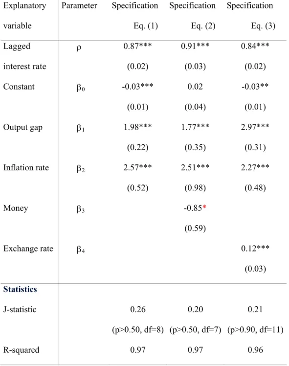
Table 2: Empirical Taylor reaction functions of the Fed GMM estimations, Quarterly data, 1999Q1-2005Q2 Explanatory variable Parameter Specification Eq. (1) Specification Eq. (2) Specification Eq. (3) Lagged interest rate ρ 0.87*** (0.02) 0.91*** (0.03) 0.84*** (0.02) Constant β0 -0.03*** (0.01) 0.02 (0.04) -0.03** (0.01) Output gap β1 1.98*** (0.22) 1.77*** (0.35) 2.97*** (0.31) Inflation rate β2 2.57*** (0.52) 2.51*** (0.98) 2.27*** (0.48) Money β3 -0.85* (0.59) Exchange rate β4 0.12*** (0.03) Statistics J-statistic 0.26 (p>0.50, df=8) 0.20 (p>0.50, df=7) 0.21 (p>0.90, df=11) R-squared 0.97 0.97 0.96

Figure 1: Short-term interest rate and Taylor rate in the euro area 2001Q3-2005Q, full-sample estimates and in-sample forecasts

.015 .020 .025 .030 .035 .040 .045 .050 01Q1 01Q3 02Q1 02Q3 03Q1 03Q3 04Q1 04Q3 05Q1 ISR_EU ISR_EU_TAYLOR _.015 .020 .025 .030 .035 .040 .045 .050 01Q1 01Q3 02Q1 02Q3 03Q1 03Q3 04Q1 04Q3 05Q1 ISR_EU ISR_EU_TAYLOR_M3 .016 .020 .024 .028 .032 .036 .040 .044 .048 01Q1 01Q3 02Q1 02Q3 03Q1 03Q3 04Q1 04Q3 05Q1 ISR_EU ISR_EU_TAYLOR_EXR

Note: One-Period-ahead in-sample forecasts based on GMM estimates. For details see footnotes to Table 1.

Figure 2: Short-term interest rate and Taylor rate in the US 2001Q3-2005Q2, full-sample estimates and in-full-sample forecasts

.01 .02 .03 .04 .05 .06 .07 01Q1 01Q3 02Q1 02Q3 03Q1 03Q3 04Q1 04Q3 05Q1 ISR_US ISR_US_TAYLOR .01 .02 .03 .04 .05 .06 .07 01Q1 01Q3 02Q1 02Q3 03Q1 03Q3 04Q1 04Q3 05Q1 ISR_US ISR_US_TAYLOR_M2 .01 .02 .03 .04 .05 .06 .07 01Q1 01Q3 02Q1 02Q3 03Q1 03Q3 04Q1 04Q3 05Q1 ISR_US ISR_US_TAYLOR_EXR

Note: One-Period-ahead in-sample forecasts based on GMM estimates. For details see footnotes to Table 1.

Figure 3: Short-term interest rate and Taylor rate in the euro area 2001M05-2005M08, Out-of-sample forecasts based on GMM estimates

.020 .024 .028 .032 .036 .040 .044 .048 .052 1999 2000 2001 2002 2003 2004 2005

ISR_EU ISR_EU_ TAYLOR_M

.020 .024 .028 .032 .036 .040 .044 .048 .052 1999 2000 2001 2002 2003 2004 2005

ISR_ EU ISR_ EU_ TA YLOR_ M3M

.020 .024 .028 .032 .036 .040 .044 .048 .052 1999 2000 2001 2002 2003 2004 2005 ISR_ EU ISR_EU_TAYLOR_EXM

Note: Out-of-sample forecasts based on GMM estimates. Estimation period is 1999M01 2001M04 for the first two figures and 1999M01 2001M05 for the last figure. For the first two figures, the forecast period amounts to 2001M05-2005M08, and for the last figure it is 2001M06-2005M08. For further details see footnotes to Table 1.

Figure 4: Short-term interest rate and Taylor rate in the US 2001M01-2005M08, out-of-sample forecasts based on GMM estimates

.01 .02 .03 .04 .05 .06 .07 1999 2000 2001 2002 2003 2004 2005 ISR_US ISR_US_TAYLOR_M .01 .02 .03 .04 .05 .06 .07 1999 2000 2001 2002 2003 2004 2005

ISR_US ISR_ US_ TAYLOR_M2M

.01 .02 .03 .04 .05 .06 .07 1999 2000 2001 2002 2003 2004 2005 ISR_US ISR_US_TAYLOR_EXM

Note: Out-of-sample forecasts based on GMM estimates. Estimation period lasts from the start of the Greenspan area August 1987 until the start of the crisis of 2000/2001 in December 2000. For details see footnotes to Table 1.

DISKUSSIONSBEITRÄGE AUS DEM INSTITUT FÜR VOLKSWIRTSCHAFTSLEHRE

DER UNIVERSITÄT HOHENHEIM

Nr. 220/2003 Walter Piesch, Ein Überblick über einige erweiterte Gini-Indices

Eigenschaften, Zusammenhänge, Interpretationen

Nr. 221/2003 Ansgar Belke, Hysteresis Models and Policy Consulting

Nr. 222/2003 Ansgar Belke and Daniel Gros, Does the ECB Follow the FED? Part II

September 11th _{and the Option Value of Waiting}

Nr. 223/2003 Ansgar Belke and Matthias Göcke, Monetary Policy (In-) Effectiveness under Uncertainty

Some Normative Implications for European Monetary Policy

Nr. 224/2003 Walter Piesch, Ein Vorschlag zur Kombination von P – und M – Indices in der Disparitätsmessung

Nr. 225/2003 Ansgar Belke, Wim Kösters, Martin Leschke and Thorsten Polleit, Challenges to ECB Credibility

Nr. 226/2003 Heinz-Peter Spahn, Zum Policy-Mix in der Europäischen Währungsunion

Nr. 227/2003 Heinz-Peter Spahn, Money as a Social Bookkeeping Device

From Mercantilism to General Equilibrium Theory

Nr. 228/2003 Ansgar Belke, Matthias Göcke and Martin Hebler, Institutional Uncertainty and European Social

Union: Impacts on Job Creation and Destruction in the CEECs.

Nr. 229/2003 Ansgar Belke, Friedrich Schneider, Privatization in Austria and other EU countries: Some theoretical

reasons and first results about the privatization proceeds.

Nr. 230/2003 Ansgar Belke, Nilgün Terzibas, Die Integrationsbemühungen der Türkei aus ökonomischer Sicht.

Nr. 231/2003 Ansgar Belke, Thorsten Polleit, 10 Argumente gegen eine

Euro-US-Dollar-Wechselkursmanipulation

Nr. 232/2004 Ansgar Belke, Kai Geisslreither and Daniel Gros, On the Relationship Between Exchange Rates and

Interest Rates: Evidence from the Southern Cone

Nr. 233/2004 Lars Wang, IT-Joint Ventures and Economic Development in China- An Applied General

Equilibrium Analysis

Nr. 234/2004 Ansgar Belke, Ralph Setzer, Contagion, Herding and Exchange Rate

Instability – A Survey

Nr. 235/2004 Gerhard Wagenhals, Tax-benefit microsimulation models for Germany: A Survey

Nr. 236/2004 Heinz-Peter Spahn, Learning in Macroeconomics and Monetary Policy:

The Case of an Open Economy

Nr. 237/2004 Ansgar Belke, Wim Kösters, Martin Leschke and Thorsten Polleit,

Nr. 239/2004 Hans Pitlik, Zur politischen Rationalität der Finanzausgleichsreform in Deutschland

Nr. 240/2004 Hans Pitlik, Institutionelle Voraussetzungen marktorientierter Reformen der Wirtschaftspolitik

Nr. 241/2004 Ulrich Schwalbe, Die Berücksichtigung von Effizienzgewinnen in der Fusionskontrolle –

Ökonomische Aspekte

Nr. 242/2004 Ansgar Belke, Barbara Styczynska, The Allocation of Power in the Enlarged ECB Governing

Council: An Assessment of the ECB Rotation Model

Nr. 243/2004 Walter Piesch, Einige Anwendungen von erweiterten Gini-Indices Pk und Mk

Nr. 244/2004 Ansgar Belke, Thorsten Polleit, Dividend Yields for Forecasting Stock Market Returns

Nr. 245/2004 Michael Ahlheim, Oliver Frör, Ulrike Lehr, Gerhard Wagenhals and Ursula Wolf, Contingent

Valuation of Mining Land Reclamation in East Germany

Nr. 246/2004 Ansgar Belke and Thorsten Polleit, A Model for Forecasting Swedish Inflation

Nr. 247/2004 Ansgar Belke, Turkey and the EU: On the Costs and Benefits of Integrating a Small but

Dynamic Economy

Nr. 248/2004 Ansgar Belke und Ralph Setzer, Nobelpreis für Wirtschaftswissenschaften 2004 an Finn E. Kydland

und Edward C. Prescott

Nr. 249/2004 Gerhard Gröner, Struktur und Entwicklung der Ehescheidungen in Baden-Württemberg und Bayern

Nr. 250/2005 Ansgar Belke and Thorsten Polleit, Monetary Policy and Dividend Growth in Germany:

A Long-Run Structural Modelling Approach

Nr. 251/2005 Michael Ahlheim and Oliver Frör, Constructing a Preference-oriented Index of Environmental

Quality

Nr. 252/2005 Tilman Becker, Michael Carter and Jörg Naeve, Experts Playing the Traveler’s Dilemma

Nr. 253/2005 Ansgar Belke and Thorsten Polleit, (How) Do Stock Market Returns React to Monetary Policy?

An ARDL Cointegration Analysis for Germany

Nr. 254/2005 Hans Pitlik, Friedrich Schneider and Harald Strotmann, Legislative Malapportionment and the

Politicization of Germany’s Intergovernmental Transfer Systems

Nr. 255/2005 Hans Pitlik, Are Less Constrained Governments Really More Successful in Executing

Market-oriented Policy Changes?

Nr. 256/2005 Hans Pitlik, Folgt die Steuerpolitik in der EU der Logik des Steuerwettbewerbes?

Nr. 257/2005 Ansgar Belke and Lars Wang, The Degree of Openness to Intra-Regional Trade –

Towards Value-Added Based Openness Measures

Nr. 258/2005 Heinz-Peter Spahn, Wie der Monetarismus nach Deutschland kam. Zum Paradigmenwechsel der

Geldpolitik in den frühen 1970er Jahren

Nr. 259/2005 Walter Piesch, Bonferroni-Index und De Vergottini-Index. Zum 75. und 65. Geburtstag zweier fast

vergessener Ungleichheitsmaße

Nr. 262/2005 Ansgar Belke and Lars Wang, The Costs and Benefits of Monetary Integration Reconsidered: How to Measure Economic Openness

Nr. 263/2005 Ansgar Belke, Bernhard Herz and Lukas Vogel, Structural Reforms and the Exchange Rate Regime

A Panel Analysis for the World versus OECD Countries

Nr. 264/2005 Ansgar Belke, Bernhard Herz and Lukas Vogel, Structural Reforms and the Exchange Rate Regime

A Panel Analysis for the World versus OECD Countries

Nr. 265/2005 Ralph Setzer, The Political Economy of Fixed Exchange Rates: A Survival Analysis

Nr. 266/2005 Ansgar Belke and Daniel Gros, Is a Unified Macroeconomic Policy Necessarily Better for a

Common Currency Area?

Nr. 267/2005 Michael Ahlheim, Isabell Benignus und Ulrike Lehr, Glück und Staat –

Einige ordnungspolitische Aspekte des Glückspiels

Nr. 268/2005 Ansgar Belke, Wim Kösters, Martin Leschke und Thorsten Polleit, Back to the rules