Behavioral Simulation Methods in Tax Policy Analysis

(1)

This PDF is a selection from an out-of-print volume from the National Bureau

of Economic Research

Volume Title: Behavioral Simulation Methods in Tax Policy Analysis

Volume Author/Editor: Martin Feldstein, ed.

Volume Publisher: University of Chicago Press

Volume ISBN: 0-226-24084-3

Volume URL: http://www.nber.org/books/feld83-2

Publication Date: 1983

Chapter Title: National Savings, Economic Welfare, and the Structure of Taxation

Chapter Author: Alan J. Auerbach, Laurence J. Kotlikoff

Chapter URL: http://www.nber.org/chapters/c7716

Chapter pages in book: (p. 459 - 498)

(2)

13

National Savings, Economic

Welfare, and the

Structure of Taxation

Alan J. Auerbach and Laurence J. Kotlikoff

13.1 Introduction

In the course of the last century, the United States rate of net national savings as conventionally defined declined dramatically from over 20% in the 1880s to less than 8% in the 1970s. Over this same period, government expenditure rose from 7% to 22% of GNP, the size of the federal debt measured at book value excluding social security varied enormously from under 10% to over 90% of G N P in particular years, and the level and structure of taxes changed significantly. While economic theory provides qualitative predictions of the effects of these changes in government policy on national savings, the quantitative importance of these changes is little understood. This paper develops a perfect foresight general equilibrium simulation model of life-cycle savings that may be used to investigate the potential impact of a wide range of government policies on national savings and economic welfare. While the strict life- cycle model of savings has been questioned at both the theoretical (Barro 1974) and empirical (Kotlikoff and Summers 1981) levels, the strict (no bequests) life-cycle model provides an important benchmark to consider the range of savings and welfare responses to government policy in general and deficit policy in particular.

The simulation model can provide quantitative answers to a number of long-standing questions concerning the government’s influence on capital formation. These include the degree of crowding out of private invest-

Alan J . Auerbach is with the Department of Economics, Harvard University, and the National Bureau of Economic Research. Laurence J. Kotlikoff is with the Department of Economics, Yale University, and the National Bureau of Economic Research.

The authors are grateful to Jon Skinner, Christophe Chamley, and Lawrence Summers for helpful comments, to Maxim Engers, David Reitman, Jon Skinner, and Thomas Seal for excellent research assistance, and to the NBER for financial support.

(3)

460 Alan J. AuerbachILaurence J. Kotlikoff

ment by debt-financed increases in government expenditure, the dif- ferential effect on consumption of temporary versus more permanent tax cuts, the announcement effects of future changes in tax and expenditure policy, and the response to structural changes in the tax system, including both the choice of the tax base and the degree of progressivity. The model tracks the values of all economic variables along the transition path from the initial steady-state growth path t o the new steady-state growth path. Hence the model can be used to compute the exact welfare gains or losses for each age cohort associated with tax reform proposals. Finally, the simulation experiments can usefully instruct the specification of time series consumption regression models that purport to estimate how government policy alters national savings.

This paper describes the technical structure of the simulation model and the solution algorithm used to compute perfect foresight life-cycle growth paths. Four examples of potential applications of the model are briefly examined. These are an analysis of the welfare costs of capital income taxation, the incidence of the progressive income tax, the effect of fiscal policy on national savings, and the savings response of the private sector t o early announcements of future tax policy changes.

The principal findings from these applications of the model are: 1. The excess burden associated with the taxation of capital income provides some limited scope for improving the welfare of all current and future cohorts when lump-sum taxes and transfers are available. How- ever, given that lump-sum taxes and transfers are not available policy tools, “tax reform” proposals are likely to significantly reduce the welfare of some cohorts and significantly raise the welfare of others unless annual tax rates and their associated deficit levels are chosen with extreme care. 2. The intercohort allocation of the tax burden of government expenditure is a significantly more important determinant of national savings than is the structure of taxation.

3 . The long-run effect on the capital output ratio of switching from a progressive to a proportional income tax with no change in the stock of government debt is roughly 13%.

4. Short-run crowding out of private investment by balanced budget increases in government expenditure is on the order of 50 cents per dollar, while long-run crowding out is 20 cents per dollar of government expenditure.

5 . Temporary as well as more permanent tax cuts can lead to increases rather than decreases in national savings in the first few years following the enactment of the tax cut. This depends both on which taxes are cut and on which taxes are subsequently raised to finance interest payments on the associated deficit.

(4)

461 National Savings, Economic Welfare, and the Structure of Taxation

affect the national savings rate in periods prior to implementation of the legislation.

The welfare costs of capital income taxation, the effects of government deficit policy on capital formation, and the long-run incidence of alternative tax instruments are the focus of a growing body of economic literature. While understanding of these issues has been greatly enhanced in recent years, the literature remains seriously deficient with respect to a number of theoretical and empirical concerns. The next section of this paper provides a selected and brief review of this literature and points out those deficiencies that can be addressed with the model developed here. Section 13.3 develops life-cycle optimization conditions for both proportional and progressive wage, interest income, and consumption tax structures. The simulation methodology is described in this section as well. Section 13.4 examines the welfare costs of capital income taxation, distinguishing pure efficiency issues associated with the structure of taxation from the issue of intercohort redistribution. Section 13.5 discusses the effect of progressive taxation on national savings and describes the economic transition from a progressive income tax to a progressive consumption tax. Section 13.6 investigates the long- and short-run savings impact of alternative government fiscal policies including temporary and more permanent tax cuts, changes in the level of government expenditure, and early announcements of future changes in tax policy. Section 13.7 summarizes the paper and suggests areas for future research. 13.2 Selected Literature Review

The long-run welfare implications of deficit policy and the choice of the tax base have been the focus of numerous recent articles (Feldstein 1974; Boskin 1978; Auerbach 1979; Kotlikoff 1979; Summers 1981; and Brad- ford 1980). These analyses have emphasized the welfare of cohorts living in the new steady state that results from alterations in government policy; little attention has been paid to the welfare of generations alive during the transition to the new steady state. This long-run focus has obscured the true scope for Pareto-efficient tax reform; to the unwary reader it may also convey the incorrect impression that deficit policy by itself is inefficient rather than simply redistributive. As this paper demonstrates, changes in government tax and expenditure policies may entail significant redistribution between cohorts alive today and in the indefinite future. The incidence of these policies can be understood only by examining changes in the welfare of all cohorts-transition cohorts as well as cohorts living in the distant future when the economy converges to a new steady state. The pure efficiency gains from “tax reform” cannot be isolated by looking at changes in the welfare of only a selected group of cohorts, since

(5)

462 Alan J. AuerbachILaurence J. Kotlikoff

welfare changes may reflect redistribution from other cohorts as opposed to the elimination of excess burdens in the tax system.

Summers’s stimulating study represents the sole attempt to explicitly examine the welfare of transition cohorts. His simulation analysis sug- gested that proportional wage and consumption taxation can have markedly different long-run impacts despite the fact that the long-run structure of these two tax systems are identical. Summers demonstrated that the requirement that the government’s budget be balanced at each point in time implied a quite different intercohort distribution of the tax burden of financing government expenditure under the wage versus the consumption tax. While the long-run tax structures are identical under the two tax systems, the actual long-run tax rates are not.

Summers’s analysis, while suggestive of many of the findings presented here, is based on the assumption of myopic rather than rational expectations; the transition path of myopic life-cycle economies with respect to the size of the capital stock and the level of utility is likely to differ significantly from the perfect foresight rational expectations paths ana- lyzed here. In general, myopic expectation paths will exhibit too rapid a convergence to the new steady state since future general equilibrium changes in gross wage rates and rates of return are not taken into account in today’s consumption decisions; these future expected general equilibrium changes tend to dampen initial behavioral responses to exogenous changes in government policy parameters.

In addition to explicit steady state modeling, there have been a number of recent calculations of the efficiency costs of capital income taxation (Feldstein 1978; Boskin 1978; Green and Sheshinski 1979; and King 1980). While pointing out a number of the key determinants of the potential inefficiencies associated with the taxation of capital income, these analyses are deficient in four respects:

1. The calculations are partial equilibrium, assuming that gross factor returns are not affected by compensated changes in the structure of taxation; this may be a convenient expositional device but gives incorrect estimates of excess burden.

2. Very simple models of life-cycle behavior are used, in which individuals live and consume for two periods, working in the first period only. Once again, this simplification may be useful for some purposes but is certainly a poor description of actual life-cycle behavior. One problem is that the first-period labor supply assumption implies that changes in the interest rate have no impact on the present value of resources. Summers (1981) found that the size of the uncompensated elasticity of savings with respect to the interest rate depends critically on the magnitude of future labor earnings. The compensated elasticity of consumption is presumably also quite sensitive to the inclusion of future labor earnings.

(6)

3. These “triangle” calculations ignore the fact that any actual transition from one tax system to another must begin when some individuals are partway through life. While these calculations make some sense under the assumption that cohort-specific tax schedules could be introduced in switching from one tax regime to another, they make little sense under the realistic assumption that cohort-specific tax instruments are not available. The scope for Pareto-efficient tax reform may be greatly reduced when the set of alternative tax instruments is restricted to realistic, noncohort specific tax schedules.

4. These analyses study transitions between systems of proportional taxation, while both current and prospective tax systems are in fact progressive. It is not clear that a switch from a progressive income tax to a progressive tax on annual consumption would improve efficiency, even if such were the case for a switch from a proportional income tax to a proportional consumption tax. If individual consumption profiles rise with age, a progressive consumption tax implies rising marginal rates of tax on future relative to current consumption, thus mimicking a tax on capital income. Moreover, if the progressivity of each tax is chosen according to a desire to maintain a certain degree of equality in society, tax rates may be substantially more progressive under an annual consumption tax than under an income tax.

Each of these deficiencies may have an important effect on the measurement of the potential gains to society in switching from the current tax system to one that fully exempts capital income from taxation. Empirical investigations of the effects of government policy on capital formation have relied primarily on time series regression models. Feld- stein’s (1974) and Barro’s (1978) analyses of the effects of social security on savings and Boskin’s (1978) estimation of the “interest elasticity of saving” provide examples of standard time series procedures. Variables over which the government has some control such as the level of social security benefits or the current net rate of return are used in a regression explaining aggregate consumption. In addition to social security variables and the net interest rate, the candidates for “exogeneous” variables have included current disposable income, the stock of private wealth, the level of the government deficit, and the level of government expenditure.

As tests of the effects of government policy on savings in a life-cycle model, these regressions are subject to a number of criticisms.

1. The theoretical coefficients of the variables included in these regressions are functions not only of preferences but also of current and future values of capital income and consumption tax rates as well as current and future gross rates of return. Hence, even if government policy remains constant over the period of estimation, the coefficients cannot be expected to remain stable since values of the gross rate of return as well as

(7)

464 Alan J. Auerbach/Laurence J. Kotlikoff

tax rates will vary over time as the economy proceeds along its general equilibrium growth path toward a steady state.

2. Since the coefficients incorporate current and future tax rates as well as underlying intertemporal consumption preferences, the estimated coefficients cannot be used to analyze changes in government policy that will necessarily alter the time path of future tax rates and gross rates of return. This is the Lucas critique and is particularly applicable to Boskin’s (1978) study, which contemplates switching from our income tax regime to a completely different tax regime, namely a consumption tax.

3 . Total consumption is the aggregate of consumption of cohorts of different ages. Since in a life-cycle model the marginal propensity of cohorts to consume out of their total net future resources differs by age, the coefficients in the aggregate consumption regression will be unstable if the distribution of future resources changes over time. This is clearly the case for the private net worth variable in the social security regressions.

4. The regressions use proxy variables such as disposable income instead of the present value of net human wealth in the actual estimation. Since disposable income is correlated with each of the other variables in the regressions this problem of errors in the variables is likely to impart bias in each coefficient of the regression.

5 . Despite the fact that some variables included in the regression do not affect aggregate consumption linearly, linearity is forced on the data. Each of these critiques can be explored with the simulation model developed here. We intend to simulate particular policy alternatives and thereby produce “simulated” data. These data will then be used in regressions following the specifications found in the literature. The estimated coefficients will provide an indication of what economic theory actually predicts about these coefficients in a truly controlled experiment. For example, the estimated coefficients on social security wealth obtained from these regressions might well prove to be negative, while the data were obtained from a model in which social security dramatically lowers the capital stock.

13.3 The Model and Its Solution

We model the evolution over time of an economy composed of government, household, and production sectors. The household sector is, at any given time, made up of fifty-five overlapping generations of individuals. Each person lives for fifty-five years, supplying labor inelastically for the first forty-five of these years and then entering retirement.’ Members of a

1. Chamley (1980, 1981) provides a careful and extensive discussion of the welfare implications of the tax structure and public debt in an intertemporal model of altruistic behavior.

2. This is intended to model a typical household that “appears” at age twenty, retires at sixty-five, and dies at seventy-five.

(8)

given generation may differ in their endowments of human capital but are assumed to be identical in all other respects. To reflect observed wage profiles, the human capital endowment of each individual grows at a fixed rate h . The population as a whole grows at rate n.

As stated above, each household is a self-contained unit, engaging in life-cycle consumption behavior with no bequests. Because labor is supplied inelastically, the labor-leisure choice is not considered. We assume the lifetime utility of each household takes the form

where C, is the household’s consumption at the end of its tth year, and p and y are, respectively, taste parameters characterizing its pure rate of time preference (degree of “impatience”) and the inverse of the partial elasticity of substitution between any two years’ consumption. A large value of p indicates that the individual will consume a greater fraction of lifetime resources in the early years of life and would lead to a lower aggregate rate of savings. A large value of y indicates a strong desire to smooth consumption in different periods. In the extreme, when y equals infinity, the household possesses Leontief indifference curves and there is no substitution effect on consumption behavior.

The individual maximizes lifetime utility (1) subject to a budget constraint, the exact specification of which depends on the particular tax system in force. For a progressive income tax, the individual’s lifetime budget constraint is

where ti and w, are the gross payments to capital and labor at the end of year t ,

e,

is the labor supplied in year t , and TYt is the average tax rate on income faced by the household in year t.

By constructing a Lagrangean from expressions (1) and ( 2 ) , and dif- ferentiating with respect to each Ct, we obtain the first-order conditions:

where A is the Lagrange multiplier of the lifetime budget constraint, (4)

(9)

466 Alan J. AuerbachJLaurence J. Kotlikoff

and T~~ is the marginal income tax rate in year t . To understand these first-order conditions, consider first the proportional tax case, where marginal and average tax rates are the same. In this case, 8, = 1, and (3) dictates that the marginal utility of consumption in year t should equal the marginal utility of lifetime resources A times the implicit price of a dollar of year t consumption in year one dollars. With progressive taxes, Or is less than one and represents a reduction in the implicit price of year t consumption. This additional term reflects the fact that an increase in consumption in year twill reduce income from assets in all future years and thus reduce all future average tax rates.3

Combination of condition (3) for successive values off implies

This "transition equation" indicates how preferences and the tax structure interact to determine the shape of life-cycle consumption patterns. First, note that, as y grows, time preference and tax factors play a smaller role in determining the ratio of C, to C,- 1; at y = m, C, = C, - regardless of other parameter values. For finite values of y, the rate of consumption growth increases with an increase in the net interest rate and decreases with an increase in the rate of pure time preference.

It is important to remember that equation ( 5 ) determines only the shape of the consumption growth path, not its level. To obtain the latter, we apply (5) recursively to relate C , to C1 for all t , then substitute the resulting expression for C, into the budget constraint (2) to obtain the following expression for C1 in terms of lifetime resources:

is the proportion of lifetime resources consumed in the first year. ing to (2) is

For a progressive consumption tax, the budget constraint correspond-

s

[

I;

(1

+

4

-lw,e,

I = 1 s = 2

2 r = 1

2

[

s = 2 I!I (1 ++1 +7,,)Cr,

3 . The term 8, corrects for the present-value change in taxes assessed on the stream of income arising from a change in average tax rates. In a one-period setting, letting f stand for taxes and y for income, yA(T/y) = (AUAy - T/y)Ay.

(10)

where Tct is the average tax rate on consumption in year t. The conditions corresponding to (5) and (6) are

( 5 ' ) and (6')

(T,, is the marginal tax rate on consumption in year t ) . A comparison of

( 5 ) and (5') indicates that, in its influence on the consumption path, a progressive consumption tax with marginal rates increasing over time has a similar influence on the shape of the consumption path as a progressive income tax. If the progressive consumption tax is levied on annual rather than lifetime consumption, then

is

a function of C,. From (5') it is clear that T ~ ~ ? Tas ~r , z p . ~ - ~Hence the steeper the growth of consumption in

the absence of taxes, the greater will be the relative taxation of future consumption under an annual progressive consumption tax.

Explicit presentation of the optimizing behavior of households under other tax systems is omitted since the derivation of these results from those just presented follows in a straightforward manner.

The economy's single production sector is characterized by the Cobb- Douglas production function:

(7) x = A K ; ( ( l +g)'L,)'-',

where

x,

K,, and L, are output, capital, and labor at time t , A is a scaling constant, g is an exogenous productivity growth rate, and E is the capital share of output, assumed throughout the paper to equal 0.25. Lt is simply equal to the sum of labor endowments of all individuals in the work force. K , is generated by a recursive equation that dictates that the change in the capital stock equals private plus public savings. Competitive behavior on the part of producers ensures that the gross factor returns

r,

and

w,

are equated to the marginal products of capital and labor at time t :

(11)

468 Alan J. AuerbachILaurence J. Kotlikoff

implies that the market value of capital goods always equals their repro- duction cost; i.e. adjustment of capital to the desired levels is instan- taneous.

The government in our model needs to finance a stream of consumption expenditures, labeled G,, that grows a t the same rate as population plus productivity. For simplicity, the impact of government expenditures on individual utility is not considered in the analysis. Aside from various taxes, the government has at its disposal one-period debt which is a perfect substitute for capital in household portfolios. This enables the government to save (run surpluses) and dissave (run deficits) without investing directly. If A g , is defined as the value of government's assets (taking a negative value if there is a national debt), government tax revenue at the end of period t is

(9)

where

Fyr

and

Fc,

are the aggregate average tax rates on income and consumption, respectively, calculated as weighted averages of individual average tax rates. Given the government's ability to issue and retire debt, its budget constraint relates the present value of its expenditures to the present value of its tax receipts plus the value of its initial assets: (10) A g o + r = O

[

s = O

h

( l + r , ) ] - ' R l

= r = O

?

[

s = O

h

( 1 + 4 ) ] - ' G r .

(Note that G, corresponds to a different concept from that reported in the National Income Accounts, which includes government purchase of capital goods.)

The solution method used to compute the perfect foresight general equilibrium path of the economy depends on the type of policy change being examined. In general, one may distinguish two cases. In the first, the ultimate characteristics of the economy are known, and the final steady state t o which the economy converges after the policy change is enacted may be described without reference to the economy's transition path. An example of such a policy change is the replacement of a system of income taxation with a tax on consumption, subject to year-by-year budget balance. The configuration of taxes and the government debt in the final steady state is known here. Thus it is possible to solve for the final steady state and then use our knowledge of the initial and final steady states to solve for the economy's transition path.

The second class of problems is one where a policy involves specific actions during the transition and the final steady state cannot be identified independently from the actual transition path. For example, under a

(12)

policy which specifies a ten year cut in income taxes, compensated for by concurrent increases in the national debt, with the debt per capita held constant thereafter and a new constant rate of income tax ultimately established, it is impossible to solve for this new rate without also know- ing the level of per capita debt which is established in the transition. Here, it is necessary to solve for the final steady state and transition path simultaneously.

The actual solution for the economy’s behavior over time always begins with a characterization of the initial steady state, given initial tax structure and government debt. We assume that individuals of different generations alive during this steady state correctly perceive the tax sched- ule and factor prices they will face over time, and behave optimally with respect to these conditions. We utilize a Gauss-Seidel iteration technique to solve for this equilibrium, starting with an initial guess of the capital-labor ratio ( K I L ) , deriving from each iteration a new estimate used to update our guess and continuing the procedure until a fixed point is reached. Given the method of deriving new estimates of KIL, such a fixed point corresponds to a steady-state equilibrium.

The iteration step is slightly different for each type of tax system, but the following description of how it proceeds for a progressive income tax should be instructive. (In this example, we assume each generation is composed of one representative individual. In the actual simulations, we sometimes allow cohorts to have heterogeneous members.) A schematic representation is provided in figure 13.1. In the first stage, a guess is made of the capital-labor ratio (equivalent to a guess of the capital stock, since labor supply is fixed). Given the marginal productivity equations (8a) and (8b), this yields values for the wage w and interest rate r . Combining these values with initial guesses for the paths of marginal and average tax rates over the life cycle, we apply equations (3) and ( 6 ) to obtain the life-cycle consumption plan of the representative individual C . From the definition of savings, this yields the age-asset profile A , which may be aggregated (subtracting any national debt assumed to exist) to provide a new value of the capital stock and capital-labor ratio. The age-asset profile, along with the estimates of w and r , also provides a solution for the age-income profile, which, in turn, dictates the general level at which taxes must be set (typically one parameter is varied in the tax function) to satisfy the government budget constraint and hence the new values of marginal and average tax rates faced over the life cycle, T~ and 7,,, respectively. When the initial and final values of KIL and the tax rates are the same, this implies that the steady state has been reached.

Solution for the final steady state, when this may be done separately (the first case discussed above), proceeds in a similar manner. In such a case, the transition is solved for in the following way. We assume the transition to the new steady state takes 150 years, then solve simul-

(13)

---

c---- 1

-

c

Definition A Aggregation!- K/L K/L

I

Function w,r Behavior W n a I -

-

a

A

I

L----J

Fig. 13.1 Iteration procedure: progressive income tax.

I

1 ’

- 1

I

Revenue

I

- I

Income Definition Y

-

Constraint

I

r T

v_

1-

- I

- Y p - Y

!

z y z y

I

(14)

taneously for equilibrium in each of the 150 years of the transition period under the assumption that everyone believes that after year 150 the new steady state will obtain. This solution method is necessary because each household is assumed to take the path of future prices into account in determining its behavior. Hence the equilibrium that results in later years will affect the equilibrium in earlier years. Specifically, we assume that individuals born after the transition begins know the transition path immediately and that those born before the beginning of the transition behaved up to the time of the change in government policy as if the old steady state would continue forever. At the time of the announcement of a new policy to be instituted either immediately or in the near future, existing cohorts are “born again”; they behave like members of the new generation except that their horizon is less than fifty-five years, and they possess initial assets as a result of prior accumulation. An iteration technique is used again, but here we must begin with a vector of capital stocks (one value for each year) and two matrices of tax rates (two vectors for each year). Further, we cannot simply solve for the behavior of a representative cohort, but rather must calculate the behavior of each cohort alive during the transition. This procedure, while conceptually no more difficult than that used to find the steady states, requires consider- ably more computation. As the ultimate paths converge to the final steady state well before year 150, the assumption about conditions after year 150 does not influence our results.

When the final steady state may not be calculated independently from the transition path, the two stages are combined. Rather than calculate the final steady state, we simply calculate an “augmented” transition path lasting 205 years, where the final 55 years are constrained to have the characteristics of a steady state.

13.4 The Welfare Costs of Capital Income Taxation

The ultimate impact on the economy of a change in government policy depends on three key factors. First, the intercohort allocation of the total tax burden of financing government expenditures will determine the level of tax rates and have important income effects on the consumption of particular cohorts. Second, the tax structure (choice of tax base) offers the vector of prices each generation faces. Third, preferences determine each household’s response to a change in incentives. In the case of a heterogeneous population, the intragenerational distribution of the tax burden may also be an important determinant of the growth path of the economy.

Typically, the impact of tax policy has been studied most closely in partial equilibrium, static models in which the welfare of a representative individual is evaluated under alternative tax regimes. As discussed

(15)

472 Alan J. AuerbachILaurence J. Kotlikoff

above, this approach does not permit a study of the inefficiency involved during the transition from one steady state to another, nor does it tell us about the intergenerational transfers that may accompany the transition. For such issues to be studied, one must use a model in which overlapping generations exist and the change in tax regime is not considered as an exercise in comparative statics but rather as an explicit policy change that evolves over time.

The classic study of the static type just discussed is that of Feldstein (1978), who examines the welfare gain from switching to a consumption tax or a tax on labor income alone from one on labor and interest income. As Feldstein points out, the choice between taxing labor income and taxing consumption at a constant rate sufficient to produce an equal present-value revenue yield has no effect on the path of individual behavior. Thus, if government uses debt finance to undo any differences in the timing of tax collections, there is no difference in national savings either, since both private and public consumption are identical under the two systems. All that differs is the distribution of savings between the household and government sectors, with the government saving more under a wage tax because of the earlier receipt of tax revenues.

When there is only one generation under study, it is impossible to imagine a change in individual lifetime tax burden without a concomitant change in government expenditures. However, once several generations are considered simultaneously, it is possible to allow tax burdens to be shifted across generations as the structure of taxation changes. For example, a switch from wage taxation to consumption taxation which requires not equal present-value yield per generation but rather year-by-year budget balance will change the tax burden of each generation in the transition to the new long-run steady state. To see why this is so, consider a simple model in which there is no growth in population or government expenditures and each individual lives for two periods, working only in the first and consuming only in the second. In the long run, if there is no government debt or deficit, the tax paid on consumption by each individual in his second year must equal the amount which would be paid in the first year under a wage tax. As long as the interest rate is positive, this involves a lower present value of taxes and, because relative prices are the same under the two systems, a gain in long-run utility. This result carries through to a more general model, with individuals living, working, and consuming for several years, as long as wages occur earlier in life, on average, than does consumption. Thus Summers (1981) found that, holding government revenue per year fixed, steady-state utility is substantially higher under a consumption tax than under a wage tax.

But this gain is not due to increased efficiency, since by such a criterion the two systems are equal (and completely nondistortionary with a fixed labor supply). What is occurring is a transfer from transitional genera-

(16)

tions to those in the steady state. In the simple example used above, if there were an immediate switch to a consumption tax, all generations would be better off except the first, which would pay its taxes twice and therefore be worse off. As long as the economy is not on a path which is “dynamically inefficient” in the sense that conducting such a chain transfer in reverse would make all generations better off (as would be true if the growth rate of annual tax revenues exceeded the interest rate), such steady-state differences d o not provide a fair comparison, because implicit in them is an intergenerational realignment of the tax burden.

One could respond to this problem by requiring that government debt policy be used to neutralize any such intergenerational transfers, but this may still fall short of equating the effect of consumption and wage taxation on all generations. Consider again a simple example with individuals laboring in their first period and consuming in their second, and suppose the economy initially faces a wage tax. A complete neutraliza- tion of a switch to a consumption tax would require an exemption of the first generation from consumption taxation (they have already paid the wage tax under the old system) with revenues in that year being paid for by deficit finance. Thereafter, each period’s consumption tax receipts would redeem the previous period’s debt.

However, if, for example, we extended the model to allow individuals to consume in both periods, this policy would no longer suffice, for exempting the older generation from consumption taxes would exempt the younger generation’s first-period consumption as well. Thus a complete separation of tax structure from intergenerational transfers would appear to require not only an unconstrained use of debt policy but the ability to assess age-specific tax rates as well. In the absence of such instruments, it may be impossible to go from one tax system to an “equivalent” one without having real effects on the welfare of individuals in the transition.

Constraints on the set of tax instruments limit our ability not only to move between structurally equivalent tax systems without changing the distribution of cohort welfare but also to move to a priori less distortion- ary tax structures in a Pareto-efficient manner. Indeed, use of the limited set of tax instruments themselves may generate distortions along the transition path. One example here is transition to a consumption tax, to the extent that annual consumption tax rates change during the transition. These tax rate changes will introduce distortions in the intertemporal consumption choice of affected cohorts. In such a case, it may be possible to improve the welfare of all generations, but it is not obvious what the appropriate government policy is to accomplish this, given the limitation on generation-specific tax rates. In this case, requiring that the present value of taxes be unaffected by the change in tax structure does not provide a guide to choosing a Pareto-efficient tax transaction since

(17)

474 Alan J. AuerbachILaurence J. Kotlikoff

interest rates will be changing over the transition and there is no “cor- rect” interest rate to use in the present value calculations.

We turn now to the results of some simple simulations to demonstrate some of the points just made.

In the following example, we consider the transition paths of an economy that starts at an initial steady state with a proportional wage tax of 0.2 and a proportional interest income tax of 0.4 and switches to either a pure consumption tax or a pure wage tax. The government’s budget is assumed to be balanced each year; hence annual revenues are the same in both transitions. Individual utility parameters p and y are set at 0.02 and 1, respectively. The population grows at a rate n = 0.01, while individual human capital is assumed to grow at an annual rate of h = 0.007. In addition, we assume a constant productivity growth rate of g = 0.02. The tax rates on capital and labor and the parameters n , h , andg are chosen to accord with empirically observed magnitudes, while p and y provide reasonable results for the age-consumption profile and capital-output ratio in the initial steady state. Nevertheless, the results should be seen as illustrative and specific magnitudes viewed with some care.

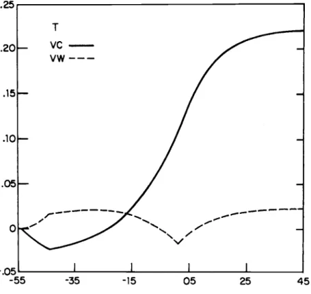
Some steady-state results of the simulation are summarized in table 13.1. From a capital-output ratio of 2.92 and a savings rate of 10% under the income tax, the economy goes to a moderately higher value of each under a wage tax (3.97 and 13.5%, respectively), but the shift to a consumption tax goes much further: the capital-output ratio is more than double under a consumption tax. It appears from these results that the change in efficiency of a tax structure may be less important in determining the characteristics of the ultimate steady state than the coincident intergenerational transfers. To see the effect of such transfers, consider figure 13.2, which presents the change in welfare for each generation between each of the two new systems and the status quo in which the income tax is kept in place. The welfare change is measured by the percentage increase or decrease in the vector of household consumption chosen under the initial tax system necessary to reach the level of utility attained under the new tax system. VC represents the gain in welfare under a consumption tax, and VW the gain under a wage tax. The Table 13.1 Income, Wage, and Consumption Taxes: Steady States

(p=.02, r = l )

Tax System

Income Wage Consumption Capital-output ratio 2.92 3.97 7.16

Gross interest rate .086 .063 ,035

Aggregate savings rate ,100 .135 ,244

(18)

horizontal axis indexes the individual generations, with generation 1 being born at the beginning of the period in which the changes are enacted. As is clear from the graph, though steady-state welfare is improved under each tax change, there are losing generations along the way. Moreover, the identity of such generations, as well as the size of the ultimate steady-state welfare gain, is very different under the two regimes.

For a switch to wage taxation, retired generations, as well as those soon to retire, gain because the bulk of their remaining income and tax liability under the income tax would be in the form of interest income and taxes on such income. Individuals born soon before or soon after the tax change are hurt. To understand why, it helps to consider the path of capital stock growth under the wage tax, relative to the baseline economy, depicted in figure 13.3 as KW. (The corresponding path for the consumption tax is labeled KC.) Note that while the capital stock is eventually 50% larger, this higher level is not reached for several years. Thus, while the added capital will eventually lead to an increase in real wages, this rise will not

-

.05

1

I

I I

1

-55 -35 -15 05 25 45

(19)

476 Alan J. Auerbach/Laurence J. Kotlikoff

T

K C

-

K W

---

100

Fig. 13.3 Capital for wage and consumption taxes.

occur immediately. Moreover, as the revenue lost from removing the interest income tax must be made up by an increase in the wage tax, net real wages decline substantially in early transition years.

The move to a consumption tax has very different effects. All generations older than twenty at the time of enactment lose, because they have paid labor income taxes when young and will now have to pay consumption taxes when old. The maximum loss of about 2.5% of lifetime resources for individuals ages forty-five at the time of enactment represents a very large loss during this cohort’s remaining years-consumption taxes are on the order of 40% in the earliest transition years, more than doubling the tax liability for such individuals relative to the old system. These losses are greater in total than those under a wage tax, but so are the eventual gains for succeeding generations. The implicit transfers from the old allow generations born as soon as five years into the transition to enjoy a 12% increase in real wealth, with an ultimate steady-state increase of 22%.

(20)

477 National Savings, Economic Welfare, and the Structure of Taxation

consumption tax might be to accept the prospect that some generations will lose and that, for any plausible discount rate applied to the gains of succeeding generations, the social gain must be quite positive. This is the argument made by Summers (1981). On the other hand, such an approach would also appear to favor a consumption tax over a wage tax, judging by the welfare comparison in figure 13.2, so it is questionable what role, if any, is being played by pure efficiency gains.

Following Phelps and Riley (1978), another way of attacking this problem is to require that other measures accompany the tax change to ensure that no generation be harmed. Without lump-sum transfers, such a policy probably requires a combination of deficit policy and the use of wage as well as consumption taxes. In figure 13.4, the welfare path of one such policy, labeled VPARETO, is presented, along with the paths VC and VW from figure 13.2. Figure 13.5 presents the corresponding capital growth paths. The policy depicted involves starting with a wage tax of 23% and a consumption tax of 9 % , gradually lowering the wage tax over fifty years to 15% while raising the consumption tax to 18%, and running

-

55 -35 -1 5 05 25 45

(21)

3.5 1 I 1 I

3 Fig. 13.5 Capital stock under a Pareto-superior plan.

deficits over the same period. The welfare path resembles that of a wage tax, except that generations older than twenty at the time of enactment gain less and all other generations do better. The use of deficit policy and wage taxation causes the capital stock t o reach a value well below that attained under a pure consumption tax.

Although this “Pareto path” is not unique, it demonstrates two important results. First, even without a full complement of instruments at the disposal of government, the long-run efficiency gains of exempting capital income from taxation are large enough to allow all generations to benefit. Of equal importance, the ultimate steady-state gain is only about one-third the gain under a pure consumption tax. Thus one may loosely attribute about two-thirds of the long-run welfare gains of switching to a consumption tax t o coincident intergenerational transfers and the re- mainder t o tax efficiency. As this result is for a model with a fixed labor supply, it is if anything an overstatement of the real efficiency gains to be had under such a change in tax regime.

(22)

13.5 Progressive Taxation

The previous section of the paper focused on the transition from a system of proportional income taxation to alternative systems of proportional taxation. In reality, the United States tax system is progressive (at least as measured by statutory tax rates) and it is likely that any new tax system would possess this characteristic as well.

In considering the additional influence of tax progressivity , we alter our existing model in a number of ways. T o facilitate the more complicated simulations necessary we ignore growth of human capital or productivity. (These parameters were found to have minor effects on the nature of transitions under proportional taxation.) As progressive taxes exist in part to mitigate the inequality of resource distribution in society, it is important to allow for the existence of heterogeneous individuals. This is accommodated in a simple manner, by assuming that each cohort has three representative individuals, with equal tastes but unequal incomes. Letting the median individual have an annual labor endowment of 1.0, the poor household is assumed to possess an endowment of 0.5, and the wealthy one an endowment of 1.5. Our final change is in the tax system itself. We replace the different systems of proportional taxation with two-parameter progressive taxes; that is, if z is the relevant tax base, we choose two parameters, labeled ci and

p,

and set the marginal tax rate equal to a

+

pz for all values of z . It follows that the corresponding average tax rate is a

+

%pz.

Setting

p

= 0 amounts to proportional taxation. Highly progressive tax systems are represented by low values of

a and high values of

p.

For the simulations of this section, the parameters from the basic proportional tax simulations above are maintained (y = 1, p = 0.02, n = 0.01); a and

p

are set equal to 0.12 and 0.14, respectively, for the progressive income tax. These values of a and

p

were obtained from a least squares regression of the marginal tax rates contained in the United States tax code, with income normalized to correspond to the levels in our simulations.

Table 13.2 gives the marginal and average tax rates which result in the steady state under progressive income taxation. For the poor person, marginal tax rates rise from 0.19 to 0.24, then dropping to 0.17 upon retirement and to 0.13 in the last year of life. The corresponding values for the median and wealthy households are (0.26, 0.34, 0.20, 0.13) and (0.33, 0.43, 0.22, 0.13), respectively. This tax structure would be expected to reduce the inequality in society, but changing marginal rates might cause inefficiencies in excess of the tax wedges introduced by equal-revenue proportional taxes. These two propositions are verified by examining the results of a switch from progressive to proportional income taxation. The poor in the long run have their real wealth (as measured above) reduced by 7.00%; the rich gain in wealth by 6.37%, and the

(23)

480 Alan J. AuerbachiLaurence J. Kotlikoff

Table 13.2 Simulated Tax Rates under Progressive Income Taxation

Poor Median Wealthy

Age MTR ATR MTR ATR MTR ATR

1 2 3 4 5 6 7 8 9 10 11 12 13 14 15 16 17 18 19 20 21 22 23 24 25 26 27 28 29 30 31 32 33 34 35 36 37 38 39 40 41 42 43 44 45 46 47 ,190 ,191 ,193 ,194 ,195 ,196 ,198 ,199 ,200 ,202 ,203 ,204 .206 ,207 .208 .210 ,211 .212 ,214 ,215 ,216 ,218 .219 .220 ,221 ,223 ,224 ,225 ,226 .227 ,228 .229 ,230 .231 ,232 ,233 .233 ,234 ,235 ,235 .236 ,236 ,236 ,237 ,237 ,167 ,164 ,155 ,156 ,156 ,157 ,158 ,158 ,159 ,160 ,160 ,161 ,162 ,162 ,163 ,164 ,164 ,165 ,166 ,166 ,167 ,168 ,168 ,169 ,169 ,170 ,171 ,171 ,172 .172 ,173 ,174 ,174 ,175 ,175 ,175 ,176 ,176 ,177 .177 ,177 ,178 ,178 ,178 .178 ,178 ,178 ,143 .142 ,260 ,262 ,264 ,267 ,269 ,271 ,273 ,275 ,277 ,280 ,282 ,284 ,286 .288 .291 ,293 ,295 .297 ,299 ,301 ,303 .305 ,307 .309 ,311 ,313 .315 ,317 ,318 ,320 ,322 ,323 ,325 .326 ,328 ,329 .330 ,332 ,333 ,334 ,335 ,335 ,336 ,337 ,337 ,198 ,193 ,190 ,191 ,192 ,193 .194 ,195 ,197 ,198 ,199 ,200 ,201 .202 ,203 ,204 ,205 ,206 ,207 ,208 .209 ,211 ,212 ,213 ,214 ,215 ,215 ,216 ,217 .218 ,219 ,220 ,221 ,222 ,222 ,223 .224 ,225 ,225 ,226 .226 ,227 .227 .228 ,228 ,228 ,229 .159 ,156 ,330 ,333 ,335 .338 ,341 .344 ,346 ,349 ,352 ,354 ,357 ,360 ,362 ,365 .367 ,370 .372 ,375 ,377 ,380 ,382 ,385 .387 ,389 ,392 ,394 ,396 ,398 ,401 ,403 ,405 ,407 ,409 ,411 ,412 ,414 .416 ,418 ,419 .421 ,422 .424 .425 ,426 ,427 ,219 .212 .225 ,226 ,228 ,229 ,230 .232 .233 ,234 ,236 .237 ,238 ,240 ,241 ,242 ,244 ,245 .246 ,247 ,249 .250 .251 ,252 ,254 ,255 ,256 ,257 ,258 .259 ,260 ,261 .262 ,263 ,264 ,265 .266 ,267 ,268 ,269 ,270 ,270 .271 ,272 ,272 .273 ,274 .170 ,166

(24)

481 National Savings, Economic Welfare, and the Structure of Taxation Table 13.2 (cont.)

Poor Median Wealthy

Age MTR ATR MTR ATR MTR ATR

48 49 50 51 52 53 54 55 ,160 ,156 .152 ,148 ,143 .138 ,132 .I26 ,140 .187 ,153 ,205 ,162 ,138 ,181 ,150 ,197 ,158 .I36 ,174 ,147 ,188 ,154 ,134 ,166 ,143 . I79 ,149 ,132 ,158 .I39 ,168 .I44 .129 ,150 ,135 ,157 ,139 ,126 ,140 ,130 ,146 ,133

.I23 .I30 .125 .I33 ,126

median group ia virtually unaffected (their wealth loss is 0.45%). This may very well represent a large loss in social welfare, taking distribution into account. However, it is clearly a gain in efficiency, since the proportional wealth gain of the rich is calculated on a much larger base than the proportional loss of the poor. This is corroborated by the fact that the long-run capital stock under progressive income taxation is 11% lower than under proportional income taxation.

Turning next to consider a switch from progressive income to progressive consumption taxes, we may ask two additional questions. First, how progressive does the consumption tax have to be to maintain the same degree of wealth inequality, measured by the Lorenz curve, as exists under a progressive income tax? Second, how is the change in steady- state utility and capital intensity between the two systems affected by the introduction of progressivity?

In answer to our first question, we find that the values of a and

p

which must be applied under a consumption tax to provide an identical Lorenz curve in the long run to that of the income tax are 0.104 and 0.432, respectively. These translate into the marginal and average tax rates listed in table 13.3. As consumption profiles rise over time, so do the tax rates of all three groups. The marginal tax rates applied to the poor person’s consumption range between 0.30 and 0.34. As these rates are fractions of consumption, it is helpful in comparing them to income tax rates to translate them into fractions of resources used for consumption (consumption plus taxes paid on such consumption). The corresponding values are 0.23 and 0.25 respectively. For median-income households, the range is 0.48 to 0.54 (0.32 t o 0.35 gross); for wealthy individuals, the range is 0.63 to 0.71 (0.39 t o 0.42, gross). Interestingly, the top (gross) marginal rax rates for the three groups are almost identical to the top rates for each under an income tax (0.25,0.35, and 0.42 versus 0.24,0.34, and 0.43).

(25)

482 Alan J. AuerbachILaurence J. Kotlikoff

Table 13.3 Simulated Tax Rates under Progressive Consumption Taxation

Poor Median Wealthy

Age MTR ATR MTR ATR MTR ATR

1 2 3 4 5 6 7 8 9 10 11 12 13 14 15 16 17 18 19 20 21 22 23 24 25 26 27 28 29 30 31 32 33 34 35 36 37 38 39 40 41 42 43 44 45 46 47 ,302 ,303 ,303 .304 ,305 ,305 ,306 .307 .307 ,308 ,309 ,309 ,310 ,311 ,311 ,312 .313 ,313 ,314 ,315 ,315 ,316 ,317 ,317 .318 ,319 .319 ,320 ,321 .321 .322 ,323 ,323 ,324 ,325 ,326 ,326 .327 ,328 ,328 ,329 ,330 ,330 ,331 ,332 ,333 ,333 ,203 .203 ,204 ,204 ,204 ,205 .205 ,205 ,206 ,206 ,206 .207 .207 ,207 ,208 ,208 ,208 ,209 ,209 ,209 ,210 ,210 ,210 ,211 ,211 ,211 ,212 ,212 ,212 .213 ,213 .213 ,214 ,214 .214 ,215 ,215 ,216 ,216 ,216 ,217 ,217 ,217 ,218 ,218 ,218 ,219 .475 .476 ,477 ,478 ,479 ,480 ,481 ,482 ,483 ,484 .486 .487 ,488 ,489 .490 ,491 ,492 ,493 ,495 .496 ,497 ,498 ,499 . 500 ,502 ,503 .SO4 .so5 ,506 ,507 SO9 ,510 ,511 .512 ,513 ,514 ,516 ,517 .518 ,519 ,520 ,522 .523 ,524 ,525 2 2 7 ,528 ,289 ,290 ,290 .291 .292 ,292 ,293 ,293 .294 ,294 ,295 ,295 ,296 .297 ,297 ,298 ,298 ,299 ,299 ,300 ,301 ,301 ,302 ,302 ,303 ,303 ,304 ,305 ,305 ,306 ,306 .307 ,307 ,308 .309 ,309 ,310 ,310 ,311 ,312 ,312 ,313 .313 ,314 .315 ,315 ,316 ,629 .630 .632 ,633 ,635 ,636 ,638 ,639 ,641 ,642 .644 ,645 ,647 ,648 ,650 .651 .653 .654 .656 ,657 ,659 ,660 .662 ,663 ,665 ,667 ,668 ,670 .671 ,673 ,674 ,676 .677 ,679 ,681 ,682 .684 ,685 .687 ,689 ,690 .692 .693 ,695 ,697 .698 ,700 ,366 ,367 ,368 ,369 ,369 .370 .371 .372 ,372 ,373 ,374 .375 ,375 ,376 ,377 .378 ,378 ,379 ,380 ,381 ,381 ,382 .383 ,384 ,385 .385 ,386 ,387 ,388 ,388 ,389 ,390 ,391 ,392 ,392 ,393 ,394 ,395 ,396 ,396 ,397 ,398 ,399 ,400 .400 ,401 .402

(26)

483 National Savings, Economic Welfare, and the Structure of Taxation Table 13.3 (cont.)

Poor Median Wealthy

Age MTR A T R MTR ATR MTR ATR

48 ,334 .219 ,529 ,317 49 ,335 ,219 ,530 ,317 50 ,335 ,220 ,531 ,318 51 ,336 ,220 ,533 ,318 52 ,337 ,221 ,534 .319 53 ,338 ,221 ,535 .320 54 ,338 ,221 ,536 .320 55 ,339 ,222 ,538 ,321 .702 ,703 .705 .706 ,708 ,710 ,711 ,713 ,403 .404 ,404 ,405 ,406 .407 ,408 ,409

In comparison to the change in capital stock under proportional taxes, a switch to consumption taxes under progressive taxation leads to a lower capital stock increase, with the capital stock going up by a factor of 3.06 in the current simulation relative to the 3.32 found above under proportional taxes. Similarly, the welfare gain is smaller. Each group in the steady state obtains a 16% increase in real wealth relative to the 22% gain under proportional taxes. These differences result because as emphasized above under progressive consumption taxes there remains an intertemporal distortion in the choice of consumption. With consumption rising over time, each household’s net rate of return is less than the gross interest rate. Our results suggest that efficiency gains of a switch may still be possible, even with the requirement that no generation be harmed, but the scope for such gains is clearly reduced by the need for tax progressivity to address the important problem of societal inequality.

13.6 The Effects of Tax Cuts, Government Expenditure, and Policy Announcements on Capital Formation

In this section, we consider the general equilibrium effects of selected fiscal policies and also examine how a switch from income taxation to the taxation of either consumption or wages would be affected by a prior announcement of such a policy.

By assumption, the government is rational and recognizes that its tax rate and expenditure paths will affect the economy’s path of labor earnings, interest income, and consumption. Hence changes in announced tax rates and expenditure levels must satisfy the government budget constraint (9) consistent with the general equilibrium changes in income and consumption such government policy choices induce.

This suggests the following important points about government policy: Temporary or permanent increases in government expenditures necessi- tate changes in the path of tax rates. The choice of which tax rates to

(27)

increase and when to increase those tax rates will determine the short-run and long-run impact of increases in government expenditure on national savings.

Temporary cuts in tax rates holding expenditures constant must be made up by increases in tax rates in the future. Again the timing and choice of future tax rate increases will influence the economic reaction to temporary

tax cuts.

Balanced budget changes in the choice of tax bases will require annual adjustments in tax rates until the economy converges to a new steady state. These annual tax changes during the transition are likely to be both inefficient in the sense of generating excess burdens and capricious in their cohort allocation of the tax burden of financing government expenditure. Announcement today of future changes in tax rates can have important implications for current revenue since the current stream of income and consumption may be affected by future tax rate policy.

13.6.1 Temporary Tax Cuts

Table 13.4 presents the effect of cuts in tax rates lasting five, ten, and twenty years on transition and long-run values of the economy’s consumption and capital output ratio. Two types of tax cuts are considered: a reduction in the proportional rate of income taxation and a reduction in the tax rate on wage income alone, holding the tax rate on capital income constant. As mentioned, temporary tax rate cuts require future tax rate increases. The simulations presented are based on the assumption that following the period of tax rate cuts the per capita debt resulting from these tax cuts is permitted from that point on to grow at the economy’s 2% rate of productivity growth. The base case with which to compare these results assumes p = 0.02 and y = 1, and a 30% proportional rate of income taxation with no initial government debt. For cuts in the proportional income tax, tax rates are reduced to 25% for the period in question. In the case of wage tax reductions, this tax rate is lowered to 23.33% for either five, ten, or twenty years; a 23.33% wage tax rate provides the same first year tax revenue reduction that is generated by cutting both wage and capital income tax rates to 25%.

Although taxes are cut initially by over 15%, table 13.4 indicates fairly small responses of aggregate consumption to tax cuts of short duration. A five year cut in the wage tax rate leads to only a 0.5% increase in consumption in the first year of the cut. The reason is simply that the majority of cohorts will end up paying for these current tax cuts in terms of higher tax rates and lower future wages after the five year period. The deficit created by this short-term tax reduction has a limited wealth effect on the economy.

4. This rules out the possibility that tax rates are so high initially that lowering them increases tax receipts.

(28)

Table 13.4 Temporary Tax Cuts

5 Year Tax Cut 10 Year Tax Cut 20 Year Tax Cut

Base Case Income Tax Wage Tax Income Tax Wage Tax Income Tax Wage Tax

Year KIY C KIY C KIY C KIY C KIY C KIY C KIY C

1 3.11 34.77 3.11 34.77 3.11 34.95 3.11 34.79 3.11 35.12 3.11 34.69 3.11 35.37 5 3.11 37.64 3.10 37.98 3.10 37.80 3.11 37.99 3.09 37.97 3.11 37.90 3.08 38.22 10 3.11 41.55 3.08 41.78 3.09 41.69 3.06 42.33 3.07 41.84 3.08 42.25 3.03 42.10 20 3.11 50.65 3.05 50.55 3.07 50.59 2.98 50.67 3.01 50.60 2.93 52.09 2.93 50.76 50 3.11 91.74 3.01 90.81 3.03 91.07 2.87 89.52 2.93 90.19 2.52 86.44 2.69 88.31 100 3.11 246.93 3.01 244.06 3.03 244.76 2.85 239.56 2.92 241.52 2.41 225.94 2.62 232.11 150 3.11 664.63 3.01 656.90 3.03 658.80 2.85 644.77 2.92 650.08 2.41 604.87 2.62 624.46

(29)

Tax cuts of longer duration have more significant effects on national savings. A twenty year wage tax cut increases aggregate consumption in the first year of the transition by 1.73% and lowers the national savings rate in year 2 from 9.40% to 8.34%. There is a 15% long-run reduction in the capital output ratio from 3.11 to 2.62; the gross wage rate falls by 5.56% in the long run, while the wage tax rate levied on this lower tax base must rise to 39% to finance interest payments on the debt as well as future government expenditures. The net wage falls therefore by 15% relative to its value in the no tax cut case.

For each of the wage tax cut simulations the long run crowding out of private capital by one dollar of government debt is approximately 52 cents. The long-run ratios of debt to capital are respectively 0.07, 0.17, and .50 for wage tax cuts of five, ten, and twenty years. The 52 cent figure reflects two facts. First, holding gross factor returns fixed, switching government tax receipts from the present to the future leads to a reduction in government savings but an increase in private savings to pay for the higher future taxes., Second, the reduction in the long-run capital stock lowers gross wages and raises gross and net interest rates; both of these factors induce greater savings.

Deficits resulting from capital as well as wage tax cuts can generate a quite different impact on capital formation in the initial phase of the tax cut. Rather than increase consumption, income tax cuts can lead to more national savings in the short run. In the twenty year income tax cut example, the first year national savings rate rises from 9.40% to 9.52%, although the long-run savings rate falls from 9.40 to 7.28%. Apparently the temporarily higher net rate of return induces a sufficiently strong savings response that the government deficit actually “crowds in” private capital. The incentives to savings are, however, only temporary. As the end of the period of tax cuts approaches, the impending higher tax rates on capital income reduce savings incentives and the income effects of the tax cut take hold. In the long run there is a smaller capital stock for deficits arising from changes in the proportional income tax rate; the long-run higher tax rate on capital income generates a permanent savings disencentive. The long-run degree of crowding out is approximately 70 cents on a dollar for each of these three cases.

13.6.2

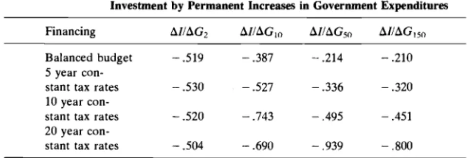
Increases in government expenditures affect capital formation directly by raising the government’s contribution to total national consumption and indirectly by altering the expected path of future tax rates. Table 13.5 describes the effect on capital formation of a 5% permanent increase in expenditures under a number of different financing scenarios. The first scenario is that the government balances its budget on an annual basis and therefore immediately raises tax rates to accommodate the increased

(30)

Table 13.5 Balanced Budget and Deficit Financed 5% Permanent Increases in Government Expenditurethe Crowding Out of National Investment by Permanent Increases in Government Expenditures Financing AllAGz AIlAGIo AlIAGSo AIIAGISO Balanced budget - ,519 - ,387 - ,214 - ,210 5 year con-

10 year con-

stant tax rates - .520 - ,743 - ,495 - ,451

20 year con-

stant tax rates - ,504 - ,690 - ,939 - ,800 Stant tax rates - ,530 - ,527 - ,336 - ,320

level of expenditures. Alternatively, the government is assumed to keep tax rates constant for five, ten, or twenty years, i.e. use deficit financing for these lengths of time. At the end of the constant tax rate interval, the government is assumed to maintain the current level or per capita debt adjusted for growth. In each case the tax rate that is adjusted is the proportional income tax rate.

Table 13.5 indicates that short-run crowding out of private investment is roughly 50 cents per dollar of government expenditure. Under the balanced budget regime, crowding out is 52 cents in the first year of the transition, it is 53 cents under the assumption of constant tax rates for five years, but it is only 50 cents for the case of constant tax rates for twenty years. In the last case, the extended period during which capital income is taxed at a lower rate promotes savings and “crowds in” an additional 2 cents of investment in the first year of the transition.

Short-run crowding out exceeds long-run crowding out in the balanced budget example for two reasons. First, even in partial equilibrium per- manently increasing the rate of proportional income taxation will alter the economy’s path of wealth accumulation; existing cohorts at the time of the tax increase hold assets that were accumulated on the basis of the previously low capital income tax rate. The initial set of elderly in particular find that at the lower net interest rate their assets are large relative to their new desired levels of future consumption. They proceed to rapidly adjust their consumption levels upward. In the long run this consumption of “excess assets” does not occur; all long-run cohorts hold assets that were accumulated from birth on the basis of the lower net return to capital. The second reason is that crowding out leads to lower long-run capital labor ratios and, in general equilibrium, higher gross and net rates of return. These higher long-run gross interest rates dampen the savings response to the higher tax rates. Although tax rates increase in the transition from 0.315 in the first year to 0.318 in year 150, the net interest rate starts out at 0.055 and rises to 0.056 because the gross interest rate increases from 0.080 to 0.082.

(31)

488 Alan J. AuerbachILaurence J. Kotlikoff

In the example of a twenty year, deficit-financed permanent increase in government expenditure, long-run crowding out is 80 cents, which exceeds short-run crowding out by 30 cents. The failure to make early elderly transition cohorts pay for any of the higher level of government expenditure leaves the economy with a lower long-run capital stock. Although consumption in year 1 is lower in the twenty year deficit case than in the balanced budget example, consumption in the twenty year deficit economy is higher in succeeding years than in the balanced budget case, and this lowers long-run capital intensity.

13.6.3 Effects of Early Announcement of Future Policy on National Savings

Early announcement of future policy