Florida International University Florida International University
FIU Digital Commons
FIU Digital Commons
FIU Electronic Theses and Dissertations University Graduate School 11-1-2018
A Mathematical Framework on Machine Learning: Theory and
A Mathematical Framework on Machine Learning: Theory and
Application
Application
Bin Shi
Florida International University, [email protected]
Follow this and additional works at: https://digitalcommons.fiu.edu/etd
Part of the Artificial Intelligence and Robotics Commons, Numerical Analysis and Computation Commons, Operational Research Commons, Ordinary Differential Equations and Applied Dynamics Commons, and the Theory and Algorithms Commons
Recommended Citation Recommended Citation
Shi, Bin, "A Mathematical Framework on Machine Learning: Theory and Application" (2018). FIU Electronic Theses and Dissertations. 3876.
https://digitalcommons.fiu.edu/etd/3876
This work is brought to you for free and open access by the University Graduate School at FIU Digital Commons. It has been accepted for inclusion in FIU Electronic Theses and Dissertations by an authorized administrator of FIU
FLORIDA INTERNATIONAL UNIVERSITY Miami, Florida
A MATHEMATICAL FRAMEWORK ON MACHINE LEARNING: THEORY AND APPLICATION
A dissertation submitted in partial fulfillment of the requirements for the degree of
DOCTOR OF PHILOSOPHY in COMPUTER SCIENCE by Bin Shi 2018
To: John L. Volakis
Dean of College of Engineering and Computing
This dissertation, written by Bin Shi, and entitled A Mathematical Framework on Machine Learning: Theory and Application, having been approved in respect to style and intellectual content, is referred to you for judgment.
We have read this dissertation and recommend that it be approved.
Leonardo Bobadilla
Zhenmin Chen
Xudong He
Jason Liu
Sundaraja S. Iyengar, Major Professor Date of Defense: September 11, 2018
The dissertation of Bin Shi is approved.
John L. Volakis Dean of College of Engineering and Computing
Andr´es G. Gil Vice President for Research and Economic Development and Dean of the University Graduate School
c
Copyright 2018 by Bin Shi All rights reserved.
DEDICATION
I dedicate this dissertation work to my beloved family, especially my parents. Without their patience, understanding, support or love, the completion of this work
ACKNOWLEDGMENTS
It is the support from many people that brings me to the completion of my dis-sertation and conclusion of my Ph.D. study.
First, I would like to express my sincerest thanks and appreciation to my ad-visors Dr.Sundaraja S. Iyengar and Dr.Tao Li, for introducing me to the field of Data Science, which is the rising interdiscipline of machine learning, optimization and statistics. With Dr.Tao Li’s success in the techniques of deep learning in practice, he was strongly aware of that the theoretical aspect is not mature by his perceptive insight. By Identifying with my strengths, he guided me into the field of theoretical development of machine learning.
Second, I would like to extend my gratitude to my major advisor, Dr. Sundaraja S. Iyengar, who has not only given huge support and encouragement for my research, but also supplied constructive suggestion in developing my Ph.D. career.
Third, my thanks to all my dissertation committee members: Dr.Xudong He, Dr.Jason Liu, Dr.Leonardo Bobadilla and Dr.Zhenmin Chen, for their helpful advice, insightful comments on my dissertation research and future research career plans.
Finally, I would like to express my utmost gratitude to my parents and family, whose endless love and understanding are with me in whatever I pursue. Without the unlimited support from them, I would never be able to survive the tough times in my life.
ABSTRACT OF THE DISSERTATION
A MATHEMATICAL FRAMEWORK ON MACHINE LEARNING: THEORY AND APPLICATION
by Bin Shi
Florida International University, 2018 Miami, Florida
Professor Sundaraja S. Iyengar, Major Professor
The dissertation addresses the research topics of machine learning outlined below. We developed the theory about traditional first-order algorithms from convex opti-mization and provide new insights in nonconvex objective functions from machine learning. Based on the theory analysis, we designed and developed new algorithms to overcome the difficulty of nonconvex objective and to accelerate the speed to obtain the desired result. In this thesis, we answer the two questions: (1) How to design a step size for gradient descent with random initialization? (2) Can we accelerate the current convex optimization algorithms and improve them into nonconvex objective? For application, we apply the optimization algorithms in sparse subspace clustering. A new algorithm, CoCoSSC, is proposed to improve the current sample complexity under the condition of the existence of noise and missing entries.
Gradient-based optimization methods have been increasingly modeled and inter-preted by ordinary differential equations (ODEs). Existing ODEs in the literature are, however, inadequate to distinguish between two fundamentally different meth-ods, Nesterov’s acceleration gradient method for strongly convex functions (NAG-SC) and Polyak’s heavy-ball method. In this paper, we derive high-resolution ODEs as more accurate surrogates for the two methods in addition to Nesterov’s acceleration gradient method for general convex functions (NAG-C), respectively. These novel
ODEs can be integrated into a general framework that allows for a fine-grained anal-ysis of the discrete optimization algorithms through translating properties of the amenable ODEs into those of their discrete counterparts. As a first application of this framework, we identify the effect of a term referred to as gradient correction in NAG-SC but not in the heavy-ball method, shedding deep insight into why the for-mer achieves acceleration while the latter does not. Moreover, in this high-resolution ODE framework, NAG-C is shown to boost the squared gradient norm minimization at the inverse cubic rate, which is the sharpest known rate concerning NAG-C itself. Finally, by modifying the high-resolution ODE of NAG-C, we obtain a family of new optimization methods that are shown to maintain the accelerated convergence rates as NAG-C for minimizing convex functions.
Key Words. Convex optimization, first-order method, Polyak’s heavy ball method, Nesterov’s accelerated gradient methods, ordinary differential equation, Lyapunov function, gradient minimization, dimensional analysis, phase space representation, numerical stability
TABLE OF CONTENTS CHAPTER PAGE 1. INTRODUCTION . . . 1 1.1 Background . . . 1 1.2 Problem Statement . . . 4 1.2.1 Optimization . . . 6
1.2.2 Online Algorithms: Sequential Updating . . . 16
1.3 Contributions . . . 19
1.3.1 Gradient Descent . . . 19
1.3.2 Accelerated Gradient Descent . . . 21
1.3.3 The CoCoSSC Method . . . 21
1.3.4 Online Time-Varying Elastic-Net Algorithm . . . 24
1.4 Organization . . . 24
2. PRELIMINARIES AND NOTATIONS . . . 25
2.1 Preliminaries and Notations . . . 25
2.2 Related Work . . . 28
3. GRADIENT DESCENT CONVERGES TO MINIMIZERS: OPTIMAL AND ADAPTIVE STEP SIZE RULES . . . 33
3.1 Maximum Allowable Step Size . . . 33
3.1.1 Consequences of Theorem 3.1.1 . . . 34
3.1.2 Optimality of Theorem 3.1.1 . . . 35
3.2 Adaptive Step Size Rules . . . 36
3.3 Proof of Theorem 3.1.1 . . . 37
3.4 Proof of Theorem 3.2.1 . . . 39
3.4.1 Hartman Product Map Theorem . . . 39
3.4.2 Complete Proof of Theorem 3.2.1 . . . 42
3.5 Appendix . . . 43
3.5.1 Additional Theorems . . . 43
3.5.2 Additional Techniques . . . 43
4. A CONSERVATION LAW METHOD IN OPTIMIZATION . . . 46
4.1 Warm-up: An Analytical Demonstration for Intuition . . . 46
4.2 Related Work . . . 48
4.3 Symplectic Scheme and Algorithms . . . 49
4.3.1 Artifically Dissipating Energy Algorithm . . . 50
4.3.2 Energy Conservation Algorithm for Detecting Local Minima . . . 53
4.3.3 Combined Algorithm . . . 55
4.4 An Asymptotic Analysis for the Phenomena of Local High-Speed Conver-gence . . . 56
4.4.1 Some Lemmas for the Linearized Scheme . . . 57
4.5 Experimental Demonstration . . . 63
4.5.1 Strongly Convex Function . . . 64
4.5.2 Non-Strongly Convex Function . . . 65
4.5.3 Non-convex Function . . . 66
5. UNDERSTANDING THE ACCELERATION PHENOMENON VIA HIGH-RESOLUTION DIFFERENTIAL EQUATIONS . . . 73
5.1 Introduction . . . 73
5.1.1 Gradient Correction: Small but Essential . . . 75
5.1.2 Overview of Contributions . . . 78
5.1.3 Related Work . . . 82
5.1.4 Organization and Notation . . . 83
5.2 The High-Resolution ODE Framework . . . 84
5.3 Gradient Correction for Acceleration . . . 90
5.3.1 The ODE Case . . . 91
5.3.2 The Discrete Case . . . 95
5.3.3 A Numerical Stability Perspective on Acceleration . . . 101
5.4 Gradient Correction for Gradient Norm Minimization . . . 103
5.4.1 The ODE Case . . . 104
5.4.2 The Discrete Case . . . 107
5.4.3 A Modified NAG-C without a Phase-Space Representation . . . 114
5.5 Extensions . . . 115
5.5.1 Convergence Rates . . . 116
5.5.2 Faster Convergence in Super-Critical Regime . . . 117
5.6 Discussion . . . 120
5.7 Technical Details and Proofs . . . 122
5.7.1 Technical Details in Section 5.2 . . . 122
5.7.2 Technical Details in Section 5.3 . . . 141
5.7.3 Technical Details in Section 5.4 . . . 153
5.7.4 Technical Details in Section 5.5 . . . 160
6. IMPROVED SAMPLE COMPLEXITY IN SPARSE SUBSPACE CLUSTER-ING WITH NOISY AND MISSCLUSTER-ING ENTRIES . . . 186
6.1 Main Results about CoCoSSC Algorithm . . . 186
6.1.1 The Non-Uniform Semi-Random Model . . . 187
6.1.2 The Fully Random Model . . . 190
6.2 Proofs . . . 190
6.2.1 Noise Characterization and Feasibility of Pre-Processing . . . 191
6.2.2 Optimality Condition and Dual Certificates . . . 191
6.2.3 Deterministic Success Conditions . . . 192
6.2.4 Bounding µeand r in Randomized Models . . . 193
6.3 Numerical results . . . 194
7. ONLINE DISCOVERY FOR STABLE AND GROUPING CAUSALITIES IN
MULTI-VARIATE TIME SERIES . . . 202
7.1 Related work . . . 202
7.2 Problem Formulation . . . 203
7.3 Elastic-net Regularizer . . . 204
7.3.1 Basic Optimization Model . . . 204
7.3.2 The Corresponding Bayesian Model . . . 205
7.3.3 Time-Varying Causal Relationship Model . . . 206
7.4 Online Inference . . . 207 7.4.1 Particle Learning . . . 208 7.4.2 Update Process . . . 209 7.4.3 Algorithm . . . 211 7.5 Empirical Study . . . 212 7.5.1 Baseline Algorithms . . . 212 7.5.2 Evaluation Metrics . . . 213
7.5.3 Synthetic Data and Experiments . . . 214
7.5.4 Climate Data and Experiments . . . 218
8. CONCLUSION . . . 223
BIBLIOGRAPHY . . . 229
LIST OF FIGURES
FIGURE PAGE
1.1 Left: Siberian Tiger; Right: South China tiger. . . 8 1.2 Left: 1; Middle: 2; Right: Mixed Gaussian:
Gaussian-1+Gaussian-2. . . 8 1.3 Left: Local Minimal Point; Middle: Local Maximal Point; Right: Saddle. 9 4.1 Minimizingf(x) = 2001 x2by the analytical solution for (4.2), (4.4) and (4.6)
with stop at the point that |v| arrive maximum, starting from x0 =
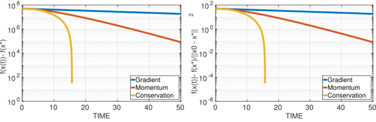
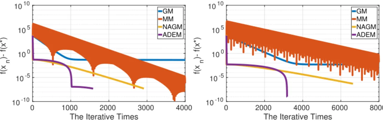
1000 and the numerical step size ∆t= 0.01. . . 47 4.2 Mimimize the function in (4.10) for artificially dissipating energy
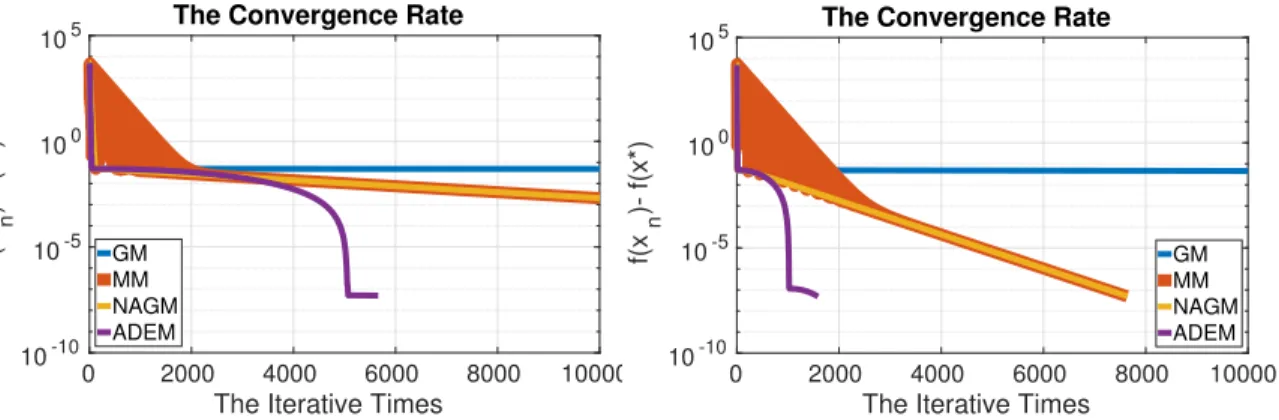
algo-rithm comparing with gradient method, momentum method and Nes-terov accelerated gradient method with stop criteria = 1e−6. The Step size: Left: h= 0.1; Right: h= 0.5. . . 51 4.3 Mimimize the function in (4.10) for artificially dissipating energy
algo-rithm comparing with gradient method, momentum method and Nes-terov accelerated gradient method with stop criteria = 1e−6. The Coefficient α: Left: α = 10−5; Right: α= 10−6. . . . 52
4.4 The trajectory for gradient method, momentum method, Nesterov ac-celerated method and artifically dissipating energy method for the function (4.10) withα = 0.1. . . 52 4.5 The Left: the step sizeh = 0.1 with 180 iterative times. The Right: the
step sizeh = 0.3 with 61 iterative times. . . 54 4.6 The common step size is seth= 0.1. The Left: the position at (2,0) with
23 iterative times. The Right: the position at (0,4) with 62 iterative times. . . 55 4.7 The Left: the case (a) with the initial point x0 = 0. The Right: the case
(b) with the initial point x0 = 1000 . . . 65
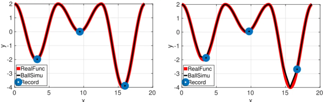
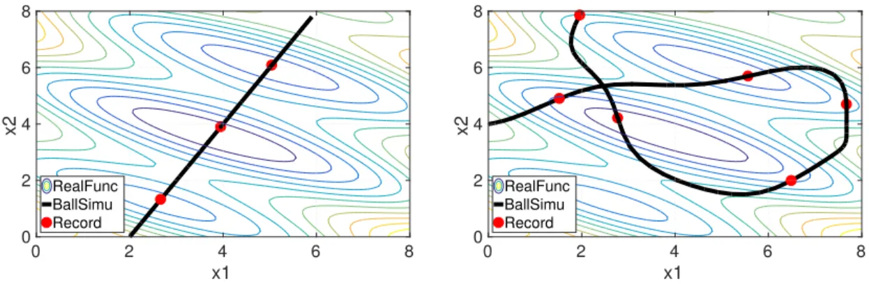
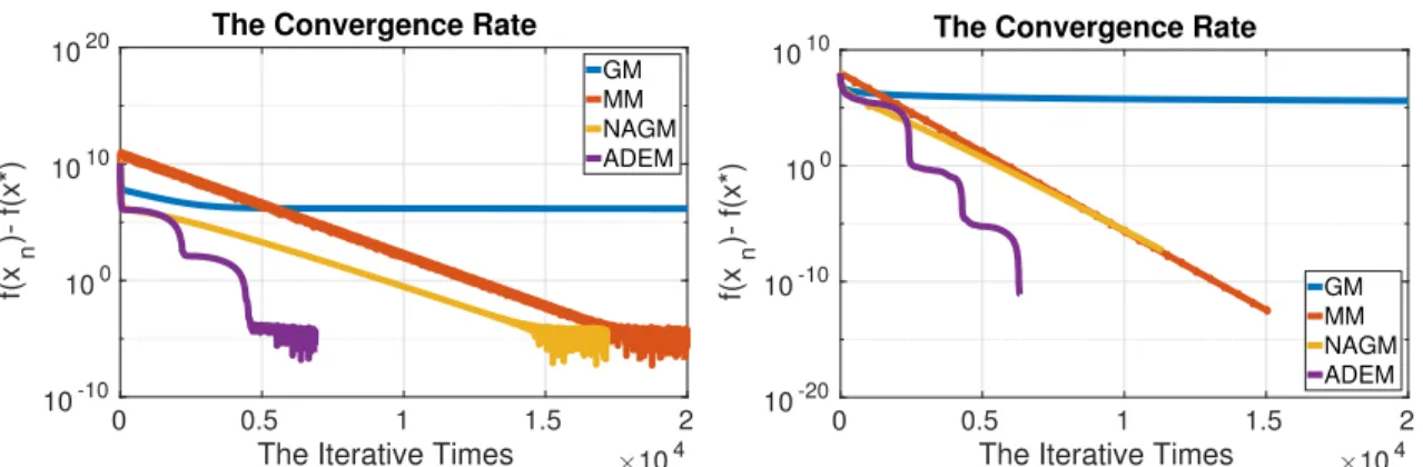
4.8 The convergence rate is shown from the initial point x0 = 0. The Left: ρ= 5; The Right: ρ= 10. . . 66 4.9 Detecting the number of the local minima of 2-D Styblinski-Tang function
by algorithm 3 with step lengthh= 0.01. The red points are recorded by algorithm 2 and the blue point are the local minima by algorithm 1. The Left: The Initial Position (5,5); The Right: The Initial Position (−5,5). . . 67 5.1 A numerical comparison between NAG-SC and heavy-ball method. The
objective function (ill-conditionedµ/L 1) isf(x1, x2) = 5×10−3x21+ x2
5.2 Top left and bottom left: trajectories and errors of NAG-SC and the heavy-ball method for minimizing f(x1, x2) = 5×10−3x21 +x22, from
the initial value (1,1), the same setting as Figure 5.1. Top right and bottom right: trajectories and errors of NAG-C for minimizing
f(x1, x2) = 2×10−2x21+ 5×10 −3x2
2, from the initial value (1,1). For
the two bottom plots, we use the identification t=k√s between time and iterations for the x-axis. . . 80 5.3 An illustration of our high-resolution ODE framework. The three solid
straight lines represent Steps 1, 2 and 3, and the two curved lines denote Step 4. The dashed line is used to emphasize that it is difficult, if not impractical, to construct discrete Lyapunov functions directly from the algorithms. . . 85 5.4 Scaled squared gradient norms2(k+ 1)3min
0≤i≤kk∇f(xi)k2 of NAG-C. In
both plots, the scaled squared gradient norm stays bounded ask → ∞. Left: f(x) = 12hAx, xi+hb, xi, where A=T0T is a 500×500 positive semidefinite matrix andb is 1×500. All entries ofb, T ∈R500×500 are
i.i.d. uniform random variables on (0,1), andk · k2 denotes the matrix
spectral norm. Right: f(x) =ρlog 200 P i=1 exp [(hai, xi −bi)/ρ] , where
A= [a1, . . . , a200]0 is a 200×50 matrix andbis a 200×1 column vector.
All entries of A and b are i.i.d.-sampled from N(0,1) and ρ= 20. . . 109 5.5 Scaled errors(k+1)2(f(x
k)−f(x?)) of the generalized NAG-C(5.57) with
various (α, β). The setting is the same as the left plot of Figure 5.4, with the objective f(x) = 12 hAx, xi+hb, xi. The step size is s = 10−1kAk−21. The left shows the short-time behaviors of the methods, while the right focuses on the long-time behaviors. The scaled error curves with the same β are very close to each other in the short-time regime, but in the long-time regime, the scaled error curves with the sameα almost overlap. The four scaled error curves slowly tend to zero.118 5.6 Scaled error s(k + 1)2(f(x
k)− f(x?)) of the generalized NAG-C (5.57)
with various (α, β). The setting is the same as the right plot of Fig-ure 5.4, with the objective f(x) = ρlog
200 P i=1 exp [(hai, xi −bi)/ρ] . The step size is s = 0.1. This set of simulation studies implies that the convergence in Theorem 5.5.3 is slow for some problems. . . 119 6.1 Heatmaps of similarity matrices {ci}Ni=1, with brighter colors indicating
larger absolute values of matrix entries. Left: LassoSSC; Middle: De-Biased Dantzig Selector; Right: CoCoSSC. . . 194 6.2 The Fowlkes-Mallows (FM) index of clustering results (top row) and
RelViolation scores (bottom row) of the three methods, with noise of magnitude σ varying from 0 to 1. Left column: missing rate 1−ρ= 0.03, middle column: 1−ρ= 0.25, right column: 1−ρ= 0.9. 196
7.1 The temporal dependency identification performance is evaluated in terms of AUC and prediction error for algorithmsBLR(1.0)BLasso(1k),TVLR(1.0),
TVLasso(1k, 2k),TVElastic-Net(1k, 2k, 1m, 2m). The bucket size is 200. . . 215 7.2 The temporal dependencies from 20 time series are learned and eight
coefficients among all are selected for demonstration. Coefficients with zero values are displayed in (a), (b), (e) and (f). The coefficients with periodic change, piecewise constant, constant, and random walk are shown in (c), (d), (g) and (h), respectively. . . 216 7.3 The zero point s change with time between TVLasso and TVEN. The
penalty parameters are λ1 =λ2 = 1000 for TVLasso andλ11=λ12 = λ21 =λ22= 1000 for TVEN. . . 218
7.4 Average predicted value of the normalized air temperature on the total 46 grids of East Florida. . . 219 7.5 Group dependencies of air temperatures over time for two target
loca-tions. Subfigures (a) and (c) show the geographical locations and target locations are in black. Subfigures (b) and (d) show the zero points graph for the two target locations respectively. . . 221
CHAPTER 1 INTRODUCTION
1.1
Background
With the explosive growth of data nowadays, a young and interdisciplinary field, Data Science, has emerged, which uses scientific methods, processes, algorithms and systems to extract knowledge and insights from data in various forms, both structured and unstructured. This data science field is becoming popular and needs to be developed urgently so that it can serve and guide for the industry of the society. Rigorously, applied Data Science is a “concept to unify statistics, data analysis, machine learning and their related methods” in order to ”understand and analyze actual phenomena” with data. It employs techniques and theories drawn from many fields within the context of mathematics, statistics, information science, and computer science.
Within the field of data analytics,Machine Learningis a method used to devise complex models and algorithms that lend themselves to prediction; in commercial use, this is known as predictive analytics. The name Machine Learning was coined in 1959 by Arthur Samuel, evolved from the study of pattern recognition and compu-tational learning theory in artificial intelligence. Computational Statistics, which also focuses on prediction-making through the use of computers, is a closely related field and often overlaps withMachine Learning.
The name, Computational Statistics, tells us that it is composed of two in-dispensable parts, statistics inference models as well as the corresponding algorithms implemented in computers. Based on the different kinds of hypotheses, statistics inference can be divided into two schools, frequentist inference school and Bayesian inference school. Now, we briefly describe them. Let H be a hypothesis and D be
data which may give evidence for H. The probabilities about the event are defined as below
• The priori P(H) is the probability that His true before the data is considered. • The posterior P(H|D) is the probability that H is true after the data D is
considered.
• The likelihood P (D|H) is the evidence about H provided by the data D. • P (D) is the total probability, shown as below
P (D) = X H
P(D|H)P(H)
Connecting the probabilities above is the significant Bayes’ formula in the theory of probability
P (H|D) = P(D|H)P(H)
P (D) ∼P (D|H)P (H). (1.1) whereP (D) can be calculated automatically if we have known the likelihoodP (D|H) andP (H). If we presume that some hypothesis (parameter specifying the conditional distribution of the data) is true and that the observed data is sampled from that distribution, that is,
P(H) = 1,
only using conditional distributions of data given specific hypotheses is the view of the frequentist school. However, if there is no presumption that some hypothesis (parameter specifying the conditional distribution of the data) is true, that is, there is a prior probability for the hypothesis H,
H ∼P(H),
summing up the information from the prior and likelihood is the view from the Bayesian school. Apparently, the view from the frequentist school is a special case
of the view from the Bayesian school, but the view from the Bayesian school is more comprehensive and requires more information.
Take the Gaussian distribution with known variance for the likelihood as an ex-ample. Without loss of generality, we assume the variance σ2 = 1. In other words,
the data point is viewed as a random variable X following the rule below, X∼P (x|H) = √1
2πe
−(x−µ2)2
where the hypothesis is H = {µ|µ ∈ (−∞,∞) is some fixed real number}. Let the data set be D = {xi}ni=1. The frequentist school requires to compute maximum
likelihood or maximum log-likelihood, that is argmax µ∈(−∞,∞) f(µ) = argmax µ∈(−∞,∞) logP(D|H) = argmax µ∈(−∞,∞) log n Y i=1 P(xi ∈ D|H) ! = argmax µ∈(−∞,∞) log 1 √ 2π n e− n P i=1 (xi−µ)2 2 =− argmin µ∈(−∞,∞) " 1 2 n X i=1 (xi−µ)2+nlog √ 2π # , (1.2)
which has been shown in the classical textbooks, such as [RS15]; whereas the Bayesian school requires to compute maximum posterior estimate or maximum log-posterior estimate, that is, we need to assume reasonable prior distribution
• If the prior distribution is a Gauss distributionµ∼ N(0, σ2
0), we have argmax µ∈(−∞,∞) f(µ) = argmax µ∈(−∞,∞) logP(D|H)P(H) = argmax µ∈(−∞,∞) log n Y i=1 logP (xi ∈ D|H) ! P (H) = argmax µ∈(−∞,∞) log 1 √ 2π n e− n P i=1 (xi−µ)2 2 · 1 √ 2πσ0 e− µ2 2σ20 =− argmin µ∈(−∞,∞) " 1 2 n X i=1 (xi−µ)2+ 1 2σ2 0 ·µ2+nlog√2π+ log√2πσ0 # (1.3)
• If the prior distribution is Laplace distributionµ∼ L(0, σ2 0), we have max µ∈(−∞,∞)f(µ) = argmaxµ∈(−∞,∞) logP(D|H)P(H) = argmax µ∈(−∞,∞) log n Y i=1 logP (xi ∈ D|H) ! P (H) = argmax µ∈(−∞,∞) log 1 √ 2π n e− n P i=1 (xi−µ)2 2 · 1 2σ2 0 e− |µ| σ2 0 =− argmin µ∈(−∞,∞) " 1 2 n X i=1 (xi−µ)2+ 1 σ2 0 · |µ|+nlog√2π+ log 2σ02 # (1.4)
• If the prior distribution is the mixed distribution combined with Laplace distri-bution and Gaussian distridistri-bution µ∼ M(0, σ2
0,1, σ02,2), we have argmax µ∈(−∞,∞) f(µ) = argmax µ∈(−∞,∞) logP(D|H)P(H) = argmax µ∈(−∞,∞) log n Y i=1 logP (xi ∈ D|H) ! P (H) = argmax µ∈(−∞,∞) log 1 √ 2π n e− n P i=1 (xi−µ)2 2 ·C(σ0,1, σ0,2)−1e − |µ| σ20,1− µ2 2σ20,2 =− argmin µ∈(−∞,∞) " 1 2 n X i=1 (xi−µ)2+ 1 σ2 0 · |µ|+ 1 2σ2 0,2 ·µ2 +nlog√2π+ logC(σ0,1, σ0,2) i (1.5) where C= 2√2πσ02,1σ0,2.
In summary, based on the description above, to solve this statistic problem can be transformed into an optimization problem.
1.2
Problem Statement
Based on the description on the statistics model in the previous section, we state the problems that we need to solve from two aspects. One is from the field of optimization,
the other is from samples of probability distribution. Practically, from the view of efficient algorithms in computers, the representation of the first one is the expectation-maximization (EM) algorithm. The EM algorithm is used to find (local) maximum likelihood parameters of a statistical model in cases where the equations cannot be solved directly. Typically these models involve latent variables in addition to unknown parameters and known data observations. That is, either missing values exist among the data, or the model can be formulated more simply by assuming the existence of further unobserved data points. For example, a mixture model can be described more simply by assuming that each observed data point has a corresponding unobserved data point, or latent variable, specifying the mixture component to which each data point belongs.
Finding a maximum likelihood solution typically requires taking the derivatives of the likelihood function with respect to all the unknown values, the parameters and the latent variables, and simultaneously solving the resulting equations. In statistical models with latent variables, this is usually impossible. Instead, the result is typically a set of interlocking equations in which the solution to the parameters requires the values of the latent variables and vice versa, but substituting one set of equations into the other produces an unsolvable equation.
The EM algorithm proceeds from the observation that there is a way to solve these two sets of equations numerically. One can simply pick arbitrary values for one of the two sets of unknowns, use them to estimate the second set, then use these new values to find a better estimate of the first set, and then keep alternating between the two until the resulting values both converge to fixed points. It’s not obvious that this will work, but it can be proven that in this context it does, and that the derivative of the likelihood is (arbitrarily close to) zero at that point, which in turn means that the point is either a maximum or a saddle point. In general, multiple maxima may
occur, with no guarantee that the global maximum will be found. Some likelihoods also have singularities in them, i.e., nonsensical maxima. For example, one of the solutions that may be found by EM in a mixture model involves setting one of the components to have zero variance and the mean parameter for the same component to be equal to one of the data points.
The second one is the Markov chain Monte Carlo (MCMC) method. Markov chain Monte Carlo methods are primarily used for calculating numerical approxima-tions of multi-dimensional integrals, for example in Bayesian statistics, computational physics, computational biology and computational linguistics.
In Bayesian statistics, the recent development of Markov chain Monte Carlo meth-ods has been a key step in making it possible to compute large hierarchical models that require integrations over hundreds or even thousands of unknown parameters.
In rare event sampling, they are also used for generating samples that gradually populate the rare failure region.
1.2.1
Optimization
Recall the process of finding the maximum probability, which is equivalent to the maximum log-likelihood or the maximum log-posterior estimate in essential. We describe them rigorously in statistics language as below.
• Finding the maximum likelihood (1.2) is equivalent to the expression below argmax µ∈(−∞,∞) f(µ) = − argmin µ∈(−∞,∞) " 1 2 n X i=1 (xi−µ)2 # , (1.6) which is namedlinear regression in statistics.
• Finding the maximum posterior estimate (1.3) is equivalent to the expression below argmax µ∈(−∞,∞) f(µ) =− argmin µ∈(−∞,∞) " 1 2 n X i=1 (xi−µ)2+ 1 2σ2 0 ·µ2 # , (1.7)
which is namedridge regression in statistics.
• Finding the maximum posterior estimate (1.3) is equivalent to the expression below argmax µ∈(−∞,∞) f(µ) =− argmin µ∈(−∞,∞) " 1 2 n X i=1 (xi−µ)2+ 1 σ2 0 · |µ| # , (1.8) which is namedlasso in statistics.
• Finding the maximum posterior estimate (1.3) is equivalent to the expression below argmax µ∈(−∞,∞) f(µ) = − argmin µ∈(−∞,∞) " 1 2 n X i=1 (xi−µ)2 + 1 σ2 0,1 · |µ|+ 1 2σ2 0,2 ·µ2 # , (1.9) which is namedelastic-net in statistics.
Linear regression (1.6) is considered as one of the standard models in statistics, the variants (1.7), (1.8) and (1.9) of which are viewed as linear regression with regularizers. Every regularizer has its own advantage, the advantage of ridge regression (1.7) is stability, that of lasso (1.8) is sparsity, and that of elastic-net (1.9) owns sparsity and group-effect. Especially, due to the sparse property, the lasso (1.8) become one of the most significant models in statistics.
The linear regression and its variants above can be reduced to finding a minimizer of the convex objective function without constraint:
min
x∈R f(x),
of which the corresponding high-dimension expression highly concerned in practice is min
x∈Rn f(x).
All of descriptions above are from the simple likelihood. In biology, the models above are suitable to study for a single species. Take the tigers in China for example.
Figure 1.1: Left: Siberian Tiger; Right: South China tiger.
There are two kinds of tigers in China, Siberian tiger and South China tiger (Fig-ure 1.1). If we only consider one kind of tigers, Siberian tiger or South China tiger, then we can assume the likelihood is a single Gaussian; but if we consider the total tigers in China, both Siberian tiger and South China tiger, then the likelihood is a superposition of two single Gaussian. The simple sketch in R is shown in Figure 1.2. Comparing the left two and the right one in Figure 1.2, there exists three stationary
Figure 1.2: Left: 1; Middle: 2; Right: Mixed Gaussian: Gaussian-1+Gaussian-2.
points, two local maximal points and one local minimal point. In other words, the objective function is nonconvex. The classical convex optimization algorithms, based on the principle that the local minimal point is the global minimal point, are not suitable for the original convex case. Furthermore, if the dimension of the objective
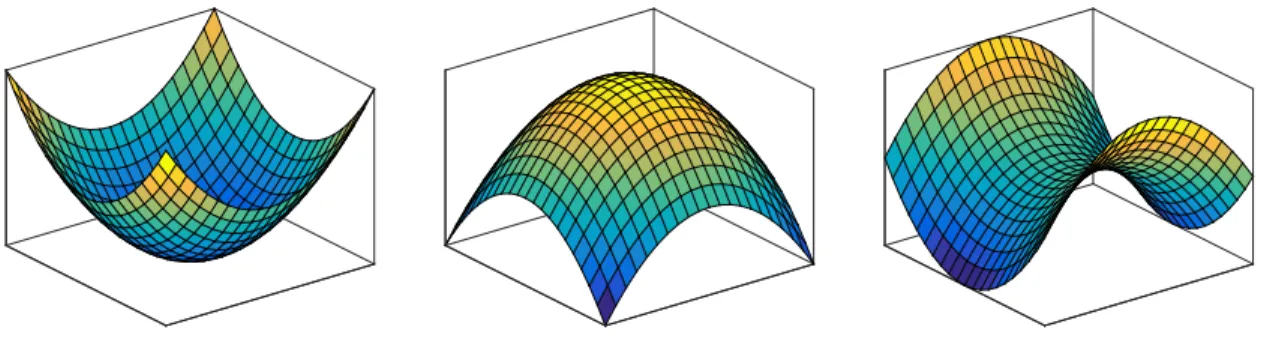
function is greater than and equal 2, there exists another stationary point: saddle. We demonstrate the different stationary points in Figure 1.3.
Figure 1.3: Left: Local Minimal Point; Middle: Local Maximal Point; Right: Saddle. From the descriptions above, many statistics models are finally transformed to solve an optimization problem, not only simple convex optimization but also complex nonconvex optimization. What’s more, the optimization algorithms are based on the information from the objective function. The classical oracle assumption for the smoothness is described in [Nes13] as below
• Zero-order oracle assumption: returns the valuef(x);
• First-order Oracle assumption: returns the valuef(x) and the gradient ∇f(x); • Second-order oracle assumption: returns the value f(x), the gradient ∇f(x)
and the Hessian∇2f(x).
To discriminate if an optimization algorithm is highly efficient in practice, based on the performance, the main characters are from oracle information and itera-tion complexity. Apparently, zero-order oracle algorithms are firstly considered. Currently, there are two main kinds of methods involved to implement: kernel-based bandit algorithms [BLE17] and algorithms of single-point gradient estima-tion [FKM05], [HL14]. Since the fewer oracle informaestima-tion leads to the higher it-eration complexity, the zero-order oracle algorithms are not popular in practice.
Furthermore, developing zero-order oracle algorithms are still in the convex stage. Second-order oracle algorithms have been studied widespread for last four decades, which are essentially based on classical Newton iteration, such as modified New-ton’s method [MS79], modified Cholesky’s method [GM74], Cubic-Regularization method [NP06] and Trust Region method [CRS14]. Currently, with the success of deep learning, some algorithms based on Hessian-prodcut in nonconvex objective have been proposed in [AAZB+17, CD16, CDHS16, LY17, RZS+17, RW17]. However, the difficulty of computing the Hessian information leads to infeasibility in current com-puters.
Now, we come to the first-order algorithms which have been widespread used. First-order algorithms only need to compute gradient which takes O(d) time com-plexity, where the dimension d is large. Recall the statistics model (1.6), (1.7), (1.8) and (1.9), if we compute the full gradient∇f(µ), it leads to deterministic algorithms; if we compute one gradient ∇fi(µ), that is, (xi −µ) for some 1 ≤ i≤ n, it leads to
stochastic algorithms. In this thesis, we focus on deterministic algorithms.
1.2.1.1 Gradient Descent
Gradient descent (GD) and its variants provide the core optimization methodology in machine learning problems. Given a C1 or C2 function f :
Rn → R with uncon-strained variable x∈Rn, GD uses the following update rule:
xk+1 =xk−hk∇f(xk) (1.10)
where hk are step size, which may be either fixed or vary across iterations. When f is convex, hk < L2 is a necessary and sufficient condition to guarantee the
(worst-case) convergence of GD, where L is the Lipschitz constant of the gradient of the function f. On the other hand, there is far less understanding of GD for non-convex
problems. For general smooth non-convex problems, GD is only known to converge to a stationary point (i.e., a point with zero gradient) [Nes13].
Machine learning tasks often require finding a local minimizer instead of just a stationary point, which can also be a saddle point or a maximizer. In recent years, there has been an increasing focus on geometric conditions under which GD escapes saddle points and converges to a local minimizer. More specifically, if the objective function satisfies 1) all saddle point are strict and 2) all local minima are global min-ima then GD finds a global optmin-imal solution. These two properties hold for a wide range of machine learning problems, such as matrix factorization [LWL+16], matrix completion [GLM16, GJZ17], matrix sensing [BNS16, PKCS17], tensor decomposi-tion [GHJY15], dicdecomposi-tionary learning [SQW17] and phase retrieval [SQW16].
Recent works showed when the objective function has the strict saddle property, then GD converges to a minimizer provided the initialization is randomized and the step sizes are fixed and smaller than 1/L [LSJR16, PP16]. While this was the first results establishing convergence of GD, there are still gaps toward fully understanding GD for strict saddle problems.
1.2.1.2 Accelerated Gradient Descent
Non-convex optimization is the dominating algorithmic technique behind many state-of-art results in machine learning, computer vision, natural language processing and reinforcement learning. Finding a global minimizer of a non-convex optimization problem is NP-hard. Instead, the local search method become increasingly important, which is based on the method from convex optimization problem. Formally, the problem of unconstrained optimization is stated in general terms as that of finding the minimum value that a function attains over Euclidean space, i.e.
min
x∈Rn f(x).
Numerous methods and algorithms have been proposed to solve the minimization problem, notably gradient methods, Newton’s methods, trust-region method, ellipsoid method and interior-point method [Pol87b, Nes13, WN99,LY+84, BV04, B+15].
First-order optimization algorithms are the most popular algorithms to perform optimization and by far the most common way to optimize neural networks, since the second-order information obtained is supremely expensive. The simplest and earliest method for minimizing a convex functionf is the gradient method, i.e.,
xk+1 =xk−h∇f(xk)
Any Initial Point : x0.
(1.11)
There are two significant improvements of the gradient method to speed up the con-vergence. One is the momentum method, named as Polyak heavy ball method, first proposed in [Pol64], i.e.,
xk+1 =xk−h∇f(xk) +γk(xk−xk−1)
Any Initial Point : x0.
(1.12)
Let κ be the condition number, which is the ratio of the smallest eigenvalue and the largest eigenvalue of Hessian at local minima. The momentum method speed up the local convergence rate from 1−2κ to 1−2√κ. The other is the Notorious Nesterov’s accelerated gradient method, first proposed in [Nes83] and an improved version [NN88, Nes13], i.e.
yk+1 =xk− 1 L∇f(xk) xk+1 =xk+γk(xk+1−xk)
Any Initial Point : x0 =y0
(1.13)
where the parameter is set as
γk =
αk(1−αk) α2k+αk+1
The scheme devised by Nesterov does not only own the property of the local con-vergence for strongly convex function, but also is the global concon-vergence scheme, from 1−2κ to 1−√κ for strongly convex function and from O 1
n to O 1 n2 for non-strongly convex function.
Although there is the complex algebraic trick in Nesterov’s accelerated gradi-ent method, the three methods above can be considered from continuous-time lim-its [Pol64, SBC14, WWJ16, WRJ16] to obtain physical intuition. In other words, the three methods can be regarded as the discrete scheme for solving the ODE. The gradient method (1.11) is correspondent to
˙ x=−∇f(xk) x(0) =x0, (1.14)
and the momentum method and Nesterov accelerated gradient method are correspon-dent to ¨ x+γtx˙+∇f(x) = 0 x(0) =x0, x˙(0) = 0, (1.15) the difference of which are the setting of the friction parameter γt. There are two
sig-nificant intuitive physical meaning in the two ODEs (1.14) and (1.15). The ODE (1.14) is the governing equation for potential flow, a correspondent phenomena of waterfall from the height along the gradient direction. The infinitesimal generalization is corre-spondent to heat conduction in nature. Hence, the gradient method (1.11) is viewed as the implement in computer or optimization simulating the phenomena in the real nature. The ODE (1.15) is the governing equation for the heavy ball motion with friction. The infinitesimal generalization is correspondent to chord vibration in na-ture. Hence, the momentum method (1.12) and the Nesterov’s accelerated gradient method (1.13) are viewed as the update version implement in computer or optimiza-tion by use of setting the fricoptimiza-tion force parameter γt.
Furthermore, we can view the three methods above as the thought for dissipating energy implemented in the computer. The unknown objective function in black box model can be viewed as the potential energy. Hence, the initial energy is from the potential functionf(x0) atx0to the minimization valuef(x?) atx?. The total energy
is combined with the kinetic energy and the potential energy. The key observation in this paper is that we find the kinetic energy, or the velocity, is observable and controllable variable in the optimization process. In other words, we can compare the velocities in every step to look for local minimum in the computational process or re-set them to zero to arrive to artificially dissipate energy.
Let us introduce firstly the governing motion equation in a conservation force field, that we use in this paper, for comparison as below,
¨ x=−∇f(x) x(0) =x0, x˙(0) = 0. (1.16)
The concept of phase space, developed in the late 19th century, usually consists of all possible values of position and momentum variables. The governing motion equation in a conservation force field (1.16) can be rewritten as
˙ x=v ˙ v =−∇f(x) x(0) =x0, v(0) = 0. (1.17)
1.2.1.3 Application to sparse subspace clustering
Subspace clustering is an important problem in machine learning, signal processing and computer vision research [Vid11]. Subspace clustering aims at grouping data points into disjoint clusters so that data points within each cluster lie near a low-dimensional linear subspace. It has found many successful applications in computer vision and machine learning, as many high dimensional data can be approximated
by a union of low-dimensional subspaces. Example data include motion trajectories [CK98], face images [BJ03], network hop counts [EBN12], movie ratings [ZFIM12] and social graphs [JCSX11].
Mathematically, let X = (x1,· · · ,xN) be an n × N data matrix, where n is
the ambient dimension and N is the number of data points. We suppose there are
L clusters S1,· · · ,SL, and each column (data point) of X belongs to exactly one
cluster, and cluster S` has N` ≤ N points in X. It is further assumed that data
points within each subspace lie approximately on a low-dimensional linear subspace U` ⊆ Rn of dimension d` n. The question is to recover the clustering of all points
inX without additional supervision.
In the case where data are noiseless (i.e., xi ∈ U` if xi belongs to cluster S`), the
following sparse subspace clustering [EV13] approach can be used:
SSC: ci := arg min
ci∈RN−1
kcik1 s.t. xi =X−ici. (1.18)
The vectors {ci}Ni=1 are usually referred to as the self-similarity matrix, or simply
similarity matrix, with the property that |cij| being large if xi and xj belong to the
same cluster and vice versa. Afterwards, spectral clustering methods can be applied on{ci}Ni=1 to produce the clustering [EV13].
While the noiseless subspace clustering model is ideal for simplified theoretical analysis, in practice data are almost always corrupted by additional noise. A general formulation for the noisy subspace clustering model is X = Y + Z where Y = (y1,· · · ,yN) is an unknown noiseless data matrix (i.e., yi ∈ U` if yi belongs to S`)
and Z = (z1,· · · ,zN) is a noise matrix such that z1,· · · ,zN are independent and
E[zi|Y] =0. Only the corrupted data matrixXis observed. Two important examples
can be formulated under this framework:
• Missing data: let Rij ∈ {0,1} be random variables indicating whether entry
Yij is observed; that is, Xij = RijYij/ρ. The noise matrix Z can be taken as
Zij = (1−Rij/ρ)Yij, where ρ > 0 is a parameter governing the probability of
observing an entry; that is, Pr[Rij = 1] =ρ.
Many methods have been proposed to cluster noisy data with subspace clustering [SEC14, WX16, QX15, Sol14]. Existing work can be categorized primarily into two formulations: the Lasso SSC formulation
Lasso SSC: ci := arg min
ci∈RN−1 kcik1+ λ 2kxi−X−icik 2 2, (1.19)
which was analyzed in [SEC14, WX16, CJW17], and a de-biased Dantzig selector approach
De-biased Dantzig Selector: ci := arg min
ci∈RN−1 kcik1+ λ 2 Σe−ici−eγi ∞ (1.20) which was proposed in [Sol14] and analyzed for an irrelevant feature setting in [QX15]. Here in Eq. (1.20) the terms Σe−i and γei are de-biased second-order statistics, defined as Σe−i =X>−iX−i−D and
e
γi =x>i X−i, where D = diag(E[z1>z1],· · · ,E[zN>zN]) is
a diagonal matrix that approximately de-biases the inner product and is assumed to be known. In particular, in the Gaussian noise model we have D = σ2I and in the
missing data model we have D = (1−ρ)2/ρ·diag(ky
1k22,· · · ,kyNk22) which can be
approximated by Db = (1−ρ)2diag(X>X) computable from corrupted data.
1.2.2
Online Algorithms: Sequential Updating
Based on the sampling methods, we here briefly introduce the principle behind the online time-varying algorithms. Let t ∈ {0,1,2, . . . , N} be a discrete finite time set. In every t ∈ {0,1,2, . . . , N}, there are always new data being observed, noted as Dt.
Recally the Bayesian formula (1.1), at timet= 0, with the prior P(H) and likelihood
P(D0|H), we have
P(H|D0)∼P(D0|H)P(H).
At timet= 1, we take the posteriorP(H|D0) at timet= 0 as the prior at timet = 1
and the likelihood P(D1|H, D0), then the new posterior att= 1 can be calculated as P(H|D0, D1)∼P(D1|H, D0)P(H|D0).
By analogy, at timet =N, we take the posteriorP(H|D0, . . . , DN−1) at timet=N−1
as the prior at timet =N and the likelihood P(DN|H, D0, . . . , DN−1), then the new
posterior at t = 1 can be calculated as
P(H|D0, . . . , DN)∼P(DN|H, D0, . . . , DN−1)P(H|D0, . . . , DN−1).
With the description above, we actually implementN+1 times maximum posterior estimate, that is, maximum posterior estimate sequence as below,
P(H|D0), P(H|D0, D1), . . . , P(H|D0, D1, DN).
In other words, obtaining the distributionP(H|D0, . . . , Dk) (k = 0, . . . , N) is
sequen-tial updating. With the probability distribution P(H|D0, . . . , Dk) at time t =k, we
can implement sampling process to generate data to observe the trend from time
t = 0 to t = N and to compare with the actual trend. Here, without any difficulty, we can find the core part of sequential updating is how to implement the likelihood sequence experimentally
P(D0|H), P(D1|H, D0), . . . , P(DN|H, D0, . . . , DN−1).
A popular technique is named as particle learning, which assume actually the likeli-hood sequence following Gaussian random walk.
1.2.2.1 Application to multivariate time series
MTS analysis has been extensively employed across diverse application domains [BJRL15, Ham94], such as finance, social network, system management, weather forecast, etc. For example, it is well-known that there exists spatial and temporal correlations be-tween air temperatures across certain regions [JHS+11, BBW+90]. Discovering and quantifying the hidden spatial-temporal dependences of the temperatures at different locations and time brings great benefits for weather forecast, especially in disaster prevention [LZZ+16].
Mining temporal dependency structure from MTS data is extensively studied across diverse domains. The Granger Causality framework is the most popular method. The intuition behind it is that if the time series A Granger causes the time series B, the future value prediction of B can be improved by giving the value ofA. Regression model has evolved to be one of the principal approaches for Granger Causality. Specifically, to predict the future value of B, one regression model built only on the past values of B should be statistically significantly less accurate than the regression model inferred by giving the past values of both A and B. Regression model with L1 regularizer [Tib96], named Lasso-Granger, is an advanced and
effec-tive approach for Granger causal relationship analysis. Lasso-Granger can effeceffec-tively identify the sparse Granger Causality especially in high dimensions [BL13].
However, Lasso-Granger suffers some essential disadvantages. The number of non-zero coefficients chosen by Lasso is bounded by the number of training instances and also it tends to randomly select only one variable and ignore the others within a vari-able group which leads to instability. Moreover, all the work described above assumes a constant dependency structure among MTS. However, this assumption rarely holds in practice, since real-world problems often involve underlying processes that are dy-namically evolving over time. Take a scenario in temperature forecast as an example.
Local temperature is usually impacted by its neighborhoods, but the dependency re-lationships dynamically change when monsoon comes from different directions. In order to capture the dynamic dependency typically happening in practice, a hidden Markov regression model [LKJ09] and a time-varying dynamic Bayesian network al-gorithm [ZWW+16] have been proposed. However, both methods infer the underlying dependency structure based on the offline mode.
1.3
Contributions
In this section, we introduce our main contributions.
1.3.1
Gradient Descent
Question 1: Maximum Allowable Fixed Step Size. Recall that for convex optimization by gradient decent with fixed step-size rule hk ≡ h, h < 2/L is both
a necessary and a sufficient condition for the convergence of GD. However, for non-convex optimization existing works all required the (fixed) step size to be smaller than 1/L. Because larger step sizes lead to faster convergence, a nature question is to identify the maximum allowable step size such that GD escapes saddle points. The main technical difficulty to analyze larger step size is that the gradient map
g(x) =x−h∇f(x)
may not be a diffeomorphism when h ≥ 1/L. Thus, techniques used in [LSJR16, PP16] are no longer sufficient.
Here, we take a finer look at the dynamics of GD. Our main observation is that the GD procedure escapes strict saddle points under much weaker conditions than g
initialization converging to a strict saddle point is 0 provided that
g(xk) =xk−ht∇f(xk)
is a local diffeomorphism at every xt. We further show that
λ({h∈[1/L,2/L) :∃t, g(xk) is not a local diffeomorphism}) = 0
whereλ(·) is the standard Lebesgue measure onR, meaning that for almost every fixed step size choice in [1/L,2/L), g(xk) is a local diffeomorphism for every t. Therefore,
if a step size h is chosen uniformly at random from L2 −,L2 for any > 0, GD escapes all strict saddle points and converges to a local minimum. See Section 3.1 for the precise statement and Section 3.3 for the proof.
Question 2: Analysis of Adaptive Step Sizes. Another open question we consider in this paper is to analyze the convergence of GD for non-convex objectives when the step sizes {ht} vary as t evolves. In convex optimization, adaptive step
size rules such as exact or backtracking line search [Nes13] are commonly used in practice to improve convergence, and convergence of GD is guaranteed provided that the adaptively tuned step sizes do not exceed twoce the inverse of local gradient Lipschitz constant. On the other hand, in non-convex optimization, whether gradient descent with varying step sizes can escape all strict saddle points is unknown.
Existing techniques [LSJR16, PP16, LPP+17, OW17] cannot solve this question because they relied on the classical Stable Manifold Theorem [Shu13], which requires a fixed gradient map whereas when step sizes vary, the gradient maps also change across iterations. To deal with this issue, we adopt the powerful Hartman product map Theorem [Har71], which gives a finer characterization of local behavior of GD and allows the gradient map to change at every iteration. Based on Hartman product map Theorem, we show that as long as the step size at each iteration is proportional to the inverse of the local gradient Lipschitz constant, GD still escapes all strict saddle
points. To our knowledge, this is the first result establishing convergence to local minima for non-convex gradient descent with varying step sizes.
1.3.2
Accelerated Gradient Descent
Here, we implement our discrete strategy into algorithms with the utility of the ob-servability and controllability of the velocity, or the kinetic energy, as well as artifi-cially dissipating energy for two directions as below,
• To look for local minima in non-convex function or global minima in convex function, the kinetic energy, or the norm of the velocity, is compared with that in the previous step, it will be re-set to zero until it becomes larger no longer. • To look for global minima in non-convex function, an initial larger velocity
v(0) = v0 is implemented at the any initial position x(0) = x0. A ball is
implemented with (1.17), the local maximum of the kinetic energy is recorded to discern how many local minima exists along the trajectory. Then implementing the strategy above to find the minimum of all the local minima.
For implementing our thought in practice, we utilize the scheme in the numerical method for Hamiltonian system, the symplectic Euler method. We remark that a more accuracy version is the St¨ormer-Verlet method for practice.
1.3.3
The CoCoSSC Method
In this paper, we consider an alternative formulation CoCoSSC to solve the noisy subspace clustering problem, inspired by theCoCoLassoestimator for high-dimensional
regression with measurement error [DZ17]. First, a pre-processing step is used that computes Σe =XTX−Db and then finds a matrix belonging to the following set:
S :=A ∈RN×N :A0 ∩nA : Ajk−Σejk ≤ |∆jk|,∀j, k ∈[N] o , (1.21)
where∆∈RN×N is an error tolerance matrix to be specified by the data analyst. For
Gaussian random noise, all entries in∆can be set to a common parameter, while for the missing data model we recommend setting two different parameters for diagonal and off-diagonal elements in ∆, as estimation errors of these elements of A behave differently under the missing data model. We give theoretical guidelines on how to set the parameters in ∆ in our main theorems, while in practice we observe that setting the elements in ∆ to be sufficiently large would normally yield good results. Because S in Eq. (1.21) is a convex set, and we will later prove that S 6=∅with high probability, a matrix Σe+ ∈S can be easily found by alternating projection fromΣ.e
For any Σe+ ∈ S and let Σe+ = XeTX, wheree Xe = ( e
x1,· · · ,xeN) ∈ R
N×N. Such a
decomposition exists because Σe+ is positive semidefinite. The self-regression vector
ci is then obtained by solving the following (convex) optimization problem:
CoCoSSC: ci := arg min
ci∈RN−1 kcik1+ λ 2 exi−Xe−ici 2 2. (1.22)
Eq. (1.22) is an `1-regularized least squares self regression problem, with the
dif-ference of usingxei andXe−i for self-regression instead of directly using the raw
noise-corrupted observations xi and X−i. This leads to improved sample complexity, as
shown in Table 1.1 and our main theorems. On the other hand, CoCoSSC retains
the nice structure of Lasso SSC, making it easier to optimize. We further discuss
this aspect and other advantages of CoCoSSCin the next section.
1.3.3.1 Advantages of CoCoSSC
The CoCoSSC has the following advantages:
1. Eq. (1.22) is easier to optimize, especially compared to the de-biased Dantzig selector approach in Eq. (1.20), because it has a smoothly differentiable objective with an `1 regularization term. Many existing methods such as ADMM [BPC+11]
can be used to obtain fast convergence. We refer the readers to [WX16, Appendix B] for further details on efficient implementation of Eq. (1.22). The pre-processing step Eq. (1.21) can also be efficiently computed using alternating projection, as both sets in Eq. (1.21) are convex. On the other hand, the de-biased Dantzig selector formulation in Eq. (1.20) is usually solved using linear programming [CT05, CT07] and could be very slow as the number of variables is large. Indeed, our empirical results show that the debiased Dantzig selector is almost 5-10 times slower than both Lasso SSC and CoCoSSC.
2. Eq. (1.22) has improved or equal sample complexity in both the Gaussian noise model and the missing data model, compared to Lasso SSC and the de-biased
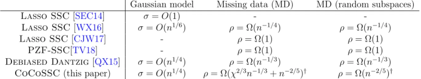
Dantzig selector. This is because a “de-biasing” pre-processing step in Eq. (1.21) is used, and an error tolerance matrix ∆ with different diagonal and off-diagonal elements is considered to reflect the heterogeneous estimation error in A. Table 1.1 gives an overview of our results and compare them with existing results. Table 1.1: Summary of success conditions with normalized signals kyik2 = 1.
Poly-nomial dependency on d, C, C and logN are omitted. In the last line χ is a sub-space affinity quantity introduced in Definition 6.1.3 for the non-uniform semi-random model. χ is always upper bounded by √d.
Gaussian model Missing data (MD) MD (random subspaces)
Lasso SSC[SEC14] σ=O(1) -
-Lasso SSC[WX16] σ=O(n1/6) ρ= Ω(n−1/4) ρ= Ω(n−1/4)
Lasso SSC[CJW17] - ρ= Ω(1) ρ= Ω(1)
PZF-SSC[TV18] - ρ= Ω(1) ρ= Ω(1)
Debiased Dantzig[QX15] σ=O(n1/4) ρ= Ω(n−1/3) ρ= Ω(n−1/3) CoCoSSC(this paper) σ=O(n1/4) ρ= Ω(χ2/3n−1/3+n−2/5)† ρ= Ω(n−2/5)†
† If ky
ik2 is exactly known, the success condition can be improved to ρ = Ω(n−1/2). See
1.3.4
Online Time-Varying Elastic-Net Algorithm
To overcome the deficiency of Lasso-Granger and capture the dynamical change of causal relationships among MTS, in this paper, we investigate the Granger Causality framework with Elasitc-Net [ZH05], which imposes a mixed L1 and L2 regularization
penalty on the linear regression. The Elastic-Net cannot only obtain strongly stable coefficients [SHB16], but also capture grouped effects of variables [SHB16, ZH05]. Furthermore, our approach explicitly models the dynamical change behaviors of the dependency as a set of random walk particles, and utilizes particle learning [CJLP10, ZWW+16] to provide a fully adaptive inference strategy which allows our model to effectively capture the varying dependency and learns the latent parameters simul-taneously. Empirical studies on both synthetic and real dataset demonstrate the effectiveness of our proposed approach.
1.4
Organization
In Chapter ??, we introduce preliminaries including notations, definitions as well as some related works. In Chapter 3, the maximum allowable step size and varying step size rules for gradient descent are shown. In Chapter 4, we show the conservation law algorithms based on accelerated gradient descent for nonconvex optimization. In Chapter 6, we introduce improved algorithm, CoCoSSC, and analyze sample complex-ity in sparse subspace Clustering with noisy and missing Entries. Finally, we show the online time-varying elastic-net algorithm to practically capture the dynamic group effect for MTS in Chapter 7.
CHAPTER 2
PRELIMINARIES AND NOTATIONS
2.1
Preliminaries and Notations
We define necessary notations and review important definitions that will be used later in our analysis. Let C2(Rn) be the vector space of real-valued twice-continuously differentiable functions. Let ∇ be the gradient operator and ∇2 be the Hessian
operator. Let k · k2 be the Euclidean norm in Rn. Let µbe the Lebesgue measure in Rn.
Definition 2.1.1 (Global Gradient Lipschitz Continuity Condition). f ∈ C2( Rn) satisfies the global gradient Lipschitz continuity condition if there exists a constant
L >0 such that
k∇f(x1)− ∇f(x2)k2 ≤Lkx1−x2k2 ∀x1, x2 ∈Rn. (2.1)
Definition 2.1.2 (Global Hessian Lipschitz Continuity Condition). f ∈C2(
Rn) sat-isfies the global Hessian Lipschitz continuity condition if there exists a constantK >0 such that ∇2f(x 1)− ∇2f(x2) 2 ≤Kkx1−x2k2 ∀x1, x2 ∈Rn. (2.2)
Intuitively, a twice-continuously differentiable function f ∈ C2(
Rn) satisfies the global gradient and Hessian Lipschitz continuity condition if its gradients and Hessians do not change dramatically for any two points in Rn. However, the global Lipschitz
constant L for many objective functions that arise in machine learning applications (e.g., f(x) = x4) may be large or even non-existent. To handle such cases, one can
use a finer definition of gradient continuity that characterizes the local behavior of gradients, especially for non-convex functions. This definition is adopted in many subjects of mathematics, such as in dynamical systems research.
Let δ > 0 be some fixed constant. For every x0 ∈ Rn, its δ-closed neighborhood is defined as
V(x0, δ) = {x∈Rn| kx−x0k2 < δ}. (2.3)
Definition 2.1.3 (Local Gradient Lipschitz Continuity Condition). f ∈C2(
Rn) sat-isfies the local gradient Lipschitz continuity condition at x0 ∈ Rn with radius δ > 0
if there exists a constant L(x0,δ)>0 such that
k∇f(x)− ∇f(y)k2 ≤L(x0,δ)kx−yk2 ∀x, y ∈V(x0, δ). (2.4)
We next review the concepts ofstationary point,local minimizer andstrict saddle point, which are important in (non-convex) optimization.
Definition 2.1.4 (Stationary Point). x∗ ∈Rn is a stationary point off ∈C2( Rn) if ∇f(x∗) = 0.
Definition 2.1.5 (Local Minimizer). x∗ ∈ Rn is a local minimum of f if there is a
neighborhood U aroundx∗ such that for all x∈U, f(x∗)< f(x).
A stationary point can be a local minimizer, a saddle point or a maximizer. It is an standard fact that if a stationary pointx? ∈
Rnis a local minimizer off ∈C2(Rn), then ∇2f(x?) is positive semidefinite; on the other hand, if x∗ ∈
Rn is a stationary point off ∈C2(
Rn) and∇2f(x?) is positive definite, thenx∗ is also a local minimizer off. It should also be noted that the stationary pointx? in the second case is isolated. The following definition concerns “strict” saddle points, which was also analyzed in [GHJY15].
Definition 2.1.6 (Strict Saddle Points). x∗ ∈Rn is astrict saddle1 of f ∈C2( Rn) if
x∗ is a stationary point of f and furthermore λmin(∇2f(x∗))<0.
We denote the set of all strict saddle points by X. By definition, a strict saddle point must have an escaping direction so that the eigenvalue of the Hessian along that direction is trictly negative. For many non-convex problems studied in machine learning, all saddle points are strict.
We next review additional concepts in multivariate analysis and differential ge-ometry/topology that will be used in our analysis.
Definition 2.1.7(Gradient Map and Its Jacobian). For anyf ∈C2(Rn), the gradient map g :Rn→Rn with step size h is defined as
g(x) =x−h∇f(x). (2.5) The JacobianDg :Rn →Rn×n of the gradient map g is defined as
Dg(x) = ∂g1 ∂x1(x) · · · ∂g1 ∂xn(x) · · · · ∂gn ∂x1(x) · · · ∂gn ∂xn(x) , (2.6) or equivalently,Dg =I−h∇2f.
We write an . bn if there exists an absolute constant C > 0 such that, for
sufficiently large n, |an| ≤ C|bn|. Similarly, an & bn if bn . an and an bn if both an . bn and bn . an are true. We write an bn if for a sufficiently small constant c >0 and sufficiently large n, |an| ≤c|bn|. For any integer M, [M] denotes the finite
set{1,2,· · · , M}.
Definition 2.1.8 (Local Diffeomorphism). LetM and N be two differentiable man-ifolds. A map f : M → N is a local diffeomorphism if for each point x in M, there exists an open set U containingx such that f(U) is open in N and f|U :U →f(U)
is a diffeomorphism.
Definition 2.1.9 (Compact Set). S ⊆Rn is compact if every open cover of S has a
Definition 2.1.10 (Sublevel Set). The α-sublevel set of f :Rn →
Ris defined as
Cα ={x∈Rn|f(x)≤α}.
2.2
Related Work
Over the past few years, there have been increasing interest in understanding the ge-ometry of non-convex programs that naturally arise from machine learning problems. It is particularly interesting to study additional properties of the considered non-convex objective such that popular optimization methods (such as gradient descent) escape saddle points and converge to a local minimum. The strict saddle property (Definition 2.1.6) is one such property. which was also shown to hold in a broad range of applications.
Many existing works leveraged Hessian information in order to circumvent saddle points This includes a modified Newton’s method [MS79], the modified Cholesky method [GM74], the cubic-regularization method [NP06] and trust region meth-ods [CRS14]. The major drawback of such second-order methods is the require-ment of access to the full Hessian, which could be computationally expensive. as the per-iteration computational complexity scales quadratically or even cubically in the problem dimension, unsuitable for optimization of high-dimensional functions. Some recent works [CDHS16, AAB+17, CD16] showed that the requirement of full Hes-sian can be relaxed to HesHes-sian-vector products, which can be computed efficiently in certain machine learning applications. Several works [LY17,RZS+17,RW17] also pre-sented algorithms that combine first-order methods with faster eigenvector algorithms to obtain lower per-iteration complexity.
Another line of works focus on noise-injected gradient methods whose per-iteration computational complexity scale linearly in the problem dimension. Earlier work have
shown that first-order method with unbiased noise with sufficiently large variance can escape strict saddle points [Pem90]. [GHJY15] gave quantitative rates on the convergence. Recently, more refined algorithms and analyses [JGN+17, JNJ17] have been proposed to improve the convergence rate of such algorithms. Nevertheless, gradient methods with deliberately injected noise are almost never used in practical applications, limiting the applicability of the above-mentioned analysis.
Empirically, [SQW16] observed that gradient descent with 100 random initializa-tions for the phase retrieval problem always converges to a local minimizer. The-oretically, the most important existing result is due to [LSJR16], who showed that gradient descent with fixed step size and any reasonable random initialization always escapes isolated strict saddle points. [PP16] later relaxed the requirement that strict saddle points are isolated. [OW17] extended the analysis to accelerated gradient de-scent and [LPP+17] generalized the result to a broader range of first-order methods, including proximal gradient descent and coordinate descent. However these works all require the step size to be significantly smaller than the inverse of Lipschitz constant of gradients, which has factor of 2 gap from results in the convex setting and do not allow the step size to vary across iterations. Our paper resolve both two problems.
The history of gradient method for convex optimization can be back to the time of Euler and Lagrange. However, since it is relatively cheaper to only calculation for first-order information, this simplest and earliest method is still active in machine learn-ing and nonconvex optimization, such as the recent work [GHJY15, AG16, LSJR16, HMR16]. The natural speedup algorithms are the momentum method first proposed in [Pol64] and Nesterov accelerated gradient method first proposed in [Nes83] and an improved version [NN88]. A acceleration algorithm similar as Nesterov accelerated gradient method, named as FISTA, is designed to solve composition problems [BT09]. A related comprehensive work is proposed in [B+15].
The original momentum method, named as Polyak heavy ball method, is from the view of ODE in [Pol64], which contains extremely rich physical intuitive ideas and mathematical theory. An extremely important work in application on machine learning is the backpropagation learning with momentum [RHW+88]. Based on the thought of ODE, a lot of understanding and application on the momentum method and Nesterov accelerated gradient methods have been proposed. In [SMDH13], a well-designed random initialization with momentum parameter algorithm is proposed to train both DNNs and RNNs. A seminal deep insight from ODE to understand the intuition behind Nesterov scheme is proposed in [SBC14]. The understanding for momentum method based on the variation perspective is proposed on [WWJ16], and the understanding from Lyaponuv analysis is proposed in [WRJ16]. From the stability theorem of ODE, the gradient method always converges to local minima in the sense of almost everywhere is proposed in [LSJR16]. Analyzing and designing iterative optimization algorithms built on integral quadratic constraints from robust control theory is proposed in [LRP16].
Actually the “high momentum” phenomenon has been firstly observed in [OC15] for a restarting adaptive accelerating algorithm, and also the restarting scheme is proposed by [SBC14]. However, both works above utilize restarting scheme for an auxiliary tool to accelerate the algorithm based on friction. With the concept of phase space in mechanics, we observe that the kinetic energy, or velocity, is controllable and utilizable parameter to find the local minima. Without friction term, we can still find the local minima only by the velocity parameter. Based on this view, the algorithm is proposed very easy to practice. Meanwhile, the thought can be generalized to nonconvex optimization to detect local minima along the trajectory of the particle.
Sparse subspace clustering was proposed by [EV13] as an effective method for sub-space clustering. [SC12] initiated the study of theoretical properties of sparse subsub-space
clustering, which was later extended to noisy data [SEC14, WX16], dimensionality-reduced data [WWS15a, HTB17, TG17] and data consisting of sensitive private in-formation [WWS15b]. [YRV15] considered some heuristics for subspace clustering with missing entries, and [TV18] considered a PZF-SSC approach and proved suc-cess conditions with ρ= Ω(1). [PCS14, HB15, LLY+13, TV17] proposed alternative approaches for subspace clustering. Some earlier references include k-plane [BM00],
q-flat [Tse00], ALC [MDHW07], LSA [YP06] and GPCA [VMS05].
It is an important task to reveal the casual dependencies between historical and current observations in MTS analysis. Bayesian Network [JYG+03, Mur02] and Granger Causality [ALA07, ZF09] are two main frameworks for inference of tem-poral dependency. Comparing with Bayesian Network, Granger Causality is more straightforward, robust and extendable [ZF09].
Originally, Granger Causality is designed for a pair of time series. The appear-ance of pioneering work of combining the notion of Granger Causality with graphical model [Eic06] leads to the emergence of causal relationship analysis among MTS data. Two typical techniques, statistical significance test and Lasso-Granger [ALA07], are developed to inference the Granger Causality among MTS. Lasso-Granger gains more popularity due to its robust performance even in high dimensions [BL12]. However, Lasso-Granger suffers from instability and failure of group variable selection because of the high sensitivity of L1 norm. To address this challenging, our method adopts
Elastic-Net regularizer [ZH05] which is stable since it encourages a group variable se-lection (group effect) where strongly correlated predictors tend to be zero or non-zero simultaneously.
Particle learning [CJLP10] is a powerful tool to provide an online inference strategy for Bayesian models. It belongs to the Sequential Monte Carlo (SMC) methods con-sisting of a set of Monte Carlo methodologies to solve the filtering problem [DGA00].
Particle learning provides state filtering, sequential parameter learning and smoothing in a general class of state space models [CJLP10]. The central idea behind particle learning is the creation of a particle algorithm that directly samples from the particle approximation to the joint posterior distribution of states and conditional sufficient statistics for fixed parameters in a fully-adapted resample-propagate framework.
CHAPTER 3
GRADIENT DESCENT CONVERGES TO MINIMIZERS: OPTIMAL AND ADAPTIVE STEP SIZE RULES
In this chapter, we first introduce our main result formally with Theo