DOI: 10.1002/sim.8569
T U T O R I A L I N B I O S T A T I S T I C S
Sensitivity analysis for clinical trials with missing
continuous outcome data using controlled multiple
imputation: A practical guide
Suzie Cro
1Tim P. Morris
2,3Michael G. Kenward
4James R. Carpenter
2,31Imperial Clinical Trials Unit, Imperial
College London, London, UK
2MRC Clinical Trials Unit at UCL, UCL,
London, UK
3Medical Statistics Department, LSHTM,
London, UK
4Ashkirk, Scotland, UK
Correspondence
Suzie Cro, Imperial Clinical Trials Unit, Imperial College London, Stadium House, 68 Wood Lane, London W12 7RH, UK. Email: [email protected]
Missing data due to loss to follow-up or intercurrent events are unintended, but unfortunately inevitable in clinical trials. Since the true values of missing data are never known, it is necessary to assess the impact of untestable and unavoid-able assumptions about any unobserved data in sensitivity analysis. This tutorial provides an overview of controlled multiple imputation (MI) techniques and a practical guide to their use for sensitivity analysis of trials with missing con-tinuous outcome data. These include 𝛿- and reference-based MI procedures. In 𝛿-based imputation, an offset term, 𝛿, is typically added to the expected value of the missing data to assess the impact of unobserved participants hav-ing a worse or better response than those observed. Reference-based imputation draws imputed values with some reference to observed data in other groups of the trial, typically in other treatment arms. We illustrate the accessibility of these methods using data from a pediatric eczema trial and a chronic headache trial and provide Stata code to facilitate adoption. We discuss issues surrounding the choice of𝛿in𝛿-based sensitivity analysis. We also review the debate on variance estimation within reference-based analysis and justify the use of Rubin's vari-ance estimator in this setting, since as we further elaborate on within, it provides
information anchoredinference.
K E Y W O R D S
clinical trials, controlled multiple imputation, missing data, multiple imputation, sensitivity analysis
1
I N T RO D U CT I O N
In late-phase clinical trials, loss to follow-up and intercurrent events—such as treatment withdrawal or partial compliance—are almost inevitable. Consequently, we often cannot measure what we intended to for all individuals. Planned outcomes may be unobtainable due to the type of the deviation (eg, missed patient visit) and, depending on the nature of the estimand and analysis, even values that were recorded post deviation may be best regarded as missing (eg, data post treatment withdrawal when an on-treatment estimand is of interest). When missing data occurs complexity arises, since any statistical analysis necessarily makes an untestable assumption about the distribution of the unobserved
This is an open access article under the terms of the Creative Commons Attribution License, which permits use, distribution and reproduction in any medium, provided the original work is properly cited.
© 2020 The Authors.Statistics in Medicinepublished by John Wiley & Sons, Ltd.
data. If the wrong assumption is made, the obtained treatment effect and its standard error will be biased, resulting in misleading inferences. To understand how far key inferences depend on the missing data assumption, analysis of incom-plete data should therefore consist not only of a primary analysis, under the most plausible missing data assumption, but include sensitivity analyses, which make a range of different credible assumptions for the unobserved data. Sensitiv-ity analysis addresses the same clinical question as the primary analysis, but under contrasting assumptions in order to assess how robust or sensitive results are Reference 1.
Regulatory guidelines from the European Medicines Agency (EMA, 2010)2 and a Food and Drug Administration
(FDA) mandated panel report from the US National Research Council (2010)3emphasize the importance of conducting
sensitivity analysis in this context. And various methods exist for conducting such sensitivity analyses in the clinical trial arena.4-6However, despite these guidelines and methodological developments, recent reviews have highlighted that
only around a third of trials with missing data are reporting sensitivity analyses.7,8This indicates a large gap between
methodological developments and practical application. The more recent publication of the ICH E9 (R1) addendum on estimands and sensitivity analysis in clinical trials (2019)9elaborates further on the importance and provides a framework
for how such sensitivity analysis should be approached. Together, these reports highlight the need for accessible and relevant methods of sensitivity analysis, where the changes in assumptions are directly applicable to the primary analysis and can be understood by key stakeholders.
One approach that enables contextually relevant accessible sensitivity analysis of clinical trials with missing data is
controlled multiple imputation(MI). Controlled MI procedures combine pattern-mixture modeling with MI to provide a practical platform for sensitivity analysis. Controlled MI procedures include𝛿-based methods, which enable one to explore the impact of a worse or better outcome than that predicted based on the individuals observed data, and the outcomes of similar patients with observed outcome data. An alternative example of controlled MI is reference-based MI, which enables one to explore the impact of individuals with missing data behaving like a specified reference group.
Such controlled MI procedures enable accessible assumptions to be explored to evaluate the impact of missing data. Furthermore, complex lengthy coding can be avoided via MI since standard statistical software packages with inbuilt MI programs can be utilized for analysis. For example,mi imputewithin Stata,proc miwithin SAS, and the R package mice. The recent increase in the discussion of controlled MI methods in the literature10-16has drawn attention to their use
for contextually relevant accessible sensitivity analysis of longitudinal trials. For examples of their use, see the analyses in References 17-20.
The purpose of this tutorial is to provide an overview of controlled MI procedures for missing data sensitivity analysis and a practical guide to their use for a continuous outcome, with worked examples and Stata code. We demonstrate the applicability and accessibility of the methods for estimating both treatment policy and hypothetical estimands. First, in Section 2, we introduce our two motivating trial case studies, which we will use to demonstrate sensitivity analysis via controlled MI. In Section 3, we discuss estimands and the problem of handling missing data within the analysis of clinical trials in more depth, followed by an outline of our general approach to primary and sensitivity analysis. This includes the necessary background on the MI procedure. We subsequently focus on the two aforementioned controlled MI approaches. The first,𝛿-based MI, is described and illustrated in Section 4. Issues around the choice of𝛿are discussed. The second controlled MI approach, reference-based MI, is described and illustrated in Section 5. We demonstrate how different assumptions for unobserved data can be readily made for different groups of individuals in the same trial analysis. In Section 6, we review the debate on variance estimation within reference-based MI analysis and justify the use of Rubin's variance estimator in this setting since, as we later further elaborate on, it providesinformation anchoredinference. We end by discussing both methods and their use within clinical trials in Section 7.
2
M OT I VAT I N G E X A M P L E S
2.1
The ADAPT trial
The Atopic Dermatitis Anti-IgE Paediatric Trial (ADAPT) was a single center, double-blind, randomized controlled trial conducted to determine whether the anti-IgE treatment, omalizumab, improves eczema severity compared to placebo in children. A total of 62 eligible children with severe eczema were randomized to treatment with omalizumab (n=30) or placebo (n=32) for 24 weeks. The trial protocol, statistical analysis plan, and main results have been previously reported.21-23In summary, significant and clinically important treatment effects at 24 weeks were reported for eczema
n=1 n=26 n=3 0 5 10 15 20 25 30 (C)DLQI 0 4 8 12 16 20 24 Time (weeks)
Mean within pattern Mean across patterns Omalizumab n=1 n=1 n=4 n=2 n=2 n=22 0 5 10 15 20 25 30 (C)DLQI 0 4 8 12 16 20 24 Time (weeks)
Mean within pattern Mean across patterns Placebo
F I G U R E 1 Observed mean profiles in the ADAPT trial [Colour figure can be viewed at wileyonlinelibrary.com]
(C)DLQI. The (C)DLQI results in a numerical score ranging between 0 and 30 (higher scores indicating worse quality of life). Data completion rates were high with only 2 participants missing week 24 follow-up for (C)DLQI in the placebo arm, who had previously withdrawn from treatment. However, 11 individuals (7 placebo 4 omalizumab) received rescue medication (alternative systemic therapy or oral steroids) sometime post week 8, up to week 24. An additional placebo patient withdrew from treatment just after week 8. Of note, two of the placebo patients who received rescue medication also withdrew from treatment thus deviated twice from the protocol.
We are interested in the treatment effect on the (C)DLQI in the absence of rescue medication/treatment withdrawal, that is, under on-treatment (hypothetical) conditions. For the purpose of our analysis, data collected post the use of rescue medication/treatment withdrawal will thus be considered missing; it is not relevant to the treatment effect or estimand of interest. Figure 1 shows the missing data patterns by treatment arm and mean (C)DLQI by missing data pattern. There are notably more deviators in the placebo arm than in the active arm.
Under on-treatment conditions, it is most plausible that the unobserved data would have been similar to the data for those with similar characteristics and (C)DLQI profile (up to time of deviation) still in the trial under on-treatment conditions. Or in other words, as we will define formally in Section 3, that the unobserved data can be considered to be missing-at-random. But we will never be certain that this assumption is true and that the results of this anal-ysis are therefore valid. It is conceivable that participants' week-24 responses could have been worse than for those observed with similar characteristics in the absence of rescue mediation. Furthermore, for those who withdrew from treatment, since they decided not to progress, it is also likely that they could have had a worse response than for those observed. In Section 4, we show how 𝛿-based MI can be used to conduct a sensitivity analysis which makes such assumptions.
2.2
Acupuncture for chronic headaches
Our second example is a multicenter randomized controlled trial conducted by Vickers et al24,25of acupuncture for chronic
headaches. A total of 401 patients with chronic headache were randomized to standard care or acupuncture and standard care for 12 months. One of the main trial outcomes was a headache score measured at baseline, 3 months and 12 months. However, not all of the randomized patients completed the 12-month follow-up. A total of 44 acupuncture participants and 56 standard care participants withdrew from the trial at or prior to 12 months. The main reasons given for withdrawal included withdrawal of consent, lost to follow-up, or intercurrent illness (see Table 4). Figure 2 shows the missing data patterns within the data. In total, 25% (100/401) of the participants were missing month 12 data.
n=39 n=17 n=4 n=136 0 5 10 15 20 25 30 35 Headache score 0 3 12 Time (months)
Mean within pattern Mean across patterns
Standard of care n=14 n=30 n=159 n=2 0 5 10 15 20 25 30 35 Headache score 0 3 12 Time (months)
Mean within pattern Mean across patterns
Acupuncture F I G U R E 2 Observed mean profiles in the acupuncture trial [Colour figure can be viewed at wileyonlinelibrary.com]
Here, we are interested in the effect of being allocated to acupuncture, that is, a treatment policy estimand, but the analysis is complicated by the unobserved data. Data are not available post trial withdrawal. As in adapt, it is most plausible that the unobserved data post trial withdrawal is missing-at-random. But it is also plausible that, following trial withdrawal, patients in the acupuncture arm experienced outcomes similar to those in the standard care arm. Figure 2 shows how on average, headache scores were slightly worse in the standard care arm at all time points. Alternatively, patients who withdrew in the control arm might subsequently have taken up acupuncture. We will explore the impact of patients behaving like those in different arms of the trial on the results in Section 5, using reference based MI. This controlled MI method is appealing since it avoids having to specify any numerical sensitivity analysis parameters; only qualitative assumptions are required.
3
A NA LY S I S W I T H M I S S I N G DATA
3.1
Estimands
In any trial, such as adapt or the acupuncture trial, we can only begin to think about missing data once we know the precise treatment effect we are aiming to estimate. Generically, the termestimandrefers to what is being estimated. Within the clinical trial context, as described in the ICH E9 addendum, an estimand refers to the precise definition of the treatment effect to be estimated to address the scientific question of interest posed by the trial's primary objective. It should capture exactly for whom, what, and when the trials intervention effect to be estimated applies, to meet the clinical goals of the trial and analysis. ICH E9 recognizes five key attributes that, when fully specified together, form a description of an estimand. These are:
(A) The population; the patients targeted by the scientific question,
(B) The treatment condition of interest and the alternative treatment condition(s), for example, control or placebo, (C) The variables (or endpoint) to be obtained for each patient required to address the scientific question,
(D) The specification of how to account for intercurrent events to reflect the scientific question of interest,
(E) The population level summary for the variable, which provides a basis for a comparison between treatment conditions.
Specification of attribute (D) is critical. For example, do we want to estimate the effect of an intervention regardless of the occurrence of intercurrent events such as treatment withdrawal or receipt of rescue medication. Such an analysis
strategy has been termed “treatment policy.” This type of estimand is of interest for the acupuncture trial. Or do we alter-natively want to estimate the effect of an intervention under hypothetical conditions, such as under ideal on-treatment conditions only. This latter hypothetical estimand is of interest in our analysis of the ADAPT trial.
The design of a trial and data collection should be aligned with the choice of estimand. For example, if we are interested in a treatment-policy estimand, we will want to ensure data collection following the occurrence of intercurrent events, such as after treatment withdrawal or use of rescue medication. If we are interested only in estimating the treatment effect under on-treatment conditions, the time and cost of data collection should be weighed against the benefit of collecting such data. If an estimand of the latter type is of interest, even if data post treatment withdrawal is collected (as in the ADAPT trial), this may be best set to missing for the purpose of analysis. Data under on-treatment conditions do not exist for the patients who withdrew from treatment or received rescue therapy following their time of withdrawal/additional treatment receipt.
The key point to re-emphasize is that we can only begin to think about missing data in any trial setting once we have fully specified the precise treatment effect we wish to estimate. The estimand should inform what data is missing for the analysis and how missing data should be handled in the analysis. Failure to collect data relevant to the estimand of interest results in a more serious missing data problem with respect to estimating the value of the estimand.
3.2
Missing data assumptions
In clinical trials, the presence of missing data creates complexity since any analysis requires us to make an assumption about the distribution of the unobserved data. Critically, this assumption is untestable. There are three broad classes of missing data assumptions originally introduced by Rubin in 1976:26Missing Completely At Random (MCAR), Missing
At Random (MAR), and Missing Not At Random (MNAR). A missingness mechanism is said to be MCAR where the probability of a datum being missing does not depend on the unobserved value of the datum, or the observed values of other recorded variables. For example, (C)DLQI data in the ADAPT trial would be MCAR if everyone in the trial had an equal probability of having their 24-week outcome recorded. Under MCAR, the marginal distribution of the unobserved data, which expresses the probability distribution of the unobserved data without reference to the values of any other variables, will be the same as the marginal distribution of the observed data. Broadly, missingness is unrelated to the inference we wish to draw.
In the more general case of MAR, the probability of a datum being missing does not depend on the unobserved value of the datum, given observed information. The missingness depends on observed data values marginally, but given the observed data is conditionally independent of the missing data values. In the ADAPT trial, if younger patients with less severe eczema at baseline were more likely to have their (C)DLQI recorded at 24 weeks, but everyone of a given age and baseline severity were equally likely to have their outcome recorded, the (C)DLQI data would be MAR. Under MAR, the marginal distribution of the unobserved data will, therefore, not be the same as the marginal distribution of the observed data, but the conditional distribution of the unobserved data given the observed data will be the same, regardless of whether the data was observed or not. Alternatively, the missingness process is termed MNAR where the probability of a datum being missing does depend on the unobserved value of the datum, even given the observed data. For example, in ADAPT, (C)DLQI would be MNAR if participants with worse (C)DLQI outcome at 24 weeks were more likely to have their 24-week (C)DLQI missing. Here, the marginal and conditional distributions of unobserved values will differ to that of the observed data.
Although MCAR can be distinguished from MAR by a comparison of covariate distributions for observed versus missing outcome values, for example, via a logistic regression, the data at hand cannot confirm which mechanism is oper-ating. Since we can never know what the missing values would have been, we cannot distinguish between MNAR and both MAR and MCAR. Sensitivity analysis thus plays a critical role to reveal the extent to which the results depend on the assumptions. In collaboration with the trial team (including those on-the-ground collecting data and clinical inves-tigators) and/or regulators, we must pick the most plausible assumption for the missing data at hand, which targets the estimand of interest, and conduct primary analysis under that assumption. Sensitivity analyses under alternative plau-sible missing data assumptions, which also target the same estimand, should subsequently be undertaken to assess the sensitivity of inferences to the underlying assumptions, including those made for missing data. Ideally, inferences would not change across sensitivity analysis, providing reassurance that the missing data did not seriously affect the interpreta-tion of results.27If this is not the case, such analysis allows individuals to assess under what conditions results change,
3.3
Approach to primary analysis
The primary analysis of a clinical trial is typically conducted under the assumption of MAR; analysis under MNAR almost always requires external information to be combined with the observed data, which is undesirable for a primary anal-ysis. MAR is a natural starting assumption for the unobserved data because it essentially states that the distribution of a patient's data at the end of the study, given their earlier observed data, does not depend on whether the data at the end of the study were observed. A version of this assumption provides a rationale for inferring that the results of a clin-ical trial will apply to individuals with similar characteristics from the population of interest not included in the trial. The strong MCAR assumption is often unlikely to be valid in the clinical trial context where drop out may be effected by treatment and observed responses. This is particularly likely in longitudinal settings when data are missing due to uncontrollable events such as receipt of rescue medication, since these events are often associated with the study vari-ables. For example, in ADAPT, it is unrealistic that (C)DLQI is missing just by chance at 24 weeks. It is more plausible that, conditional on baseline, treatment and earlier responses (which may have led to treatment withdrawal or initia-tion of rescue medicainitia-tion hence the missingness) data are MAR. Although not verifiable, MAR does not require the modeling of the dropout procedure. Under MAR, valid inference can be obtained from the likelihood of the observed data only.28 MAR will be the primary assumption made for the unobserved data in our analysis of the ADAPT and
acupuncture trial.
In practice, when data are missing, we have two accessible alternatives that provide valid inference under MAR:28,29
1. Perform a longitudinal likelihood based data analysis, which makes use of all the observed pre-deviation data from each patient, for example, a mixed model for repeated measures (MMRM);
2. Use MI and impute missing data under the primary MAR analysis assumption, fit the primary analysis model (the model of interest which would have been used in the absence of any missing data) on each imputed dataset and use Rubin's rules to combine results for inference.
The two approaches will be approximately equivalent, provided the variables used in the imputation model are the same as those included in the analysis model and conditionals are accommodated by a single joint model.30In such
set-tings, MI essentially provides an approximation to the observed likelihood analysis. If an infinite number of imputations could be performed, then the two approaches would be equivalent. In practice, the level of equivalence will depend on the number of imputations due to the Monte Carlo (simulation) sampling variability of the imputation process (described in more detail below), thus will be stronger for a larger number of imputations.31
The MI procedure can, however, be a simpler, more practical option when one wishes to include additional “ auxil-iary” information, which is predictive of missingness, within the analysis. Auxiliary variables can readily be incorporated within the imputation model but need not be conditioned on in the analysis model. This is useful when one does not want to estimate the treatment effect conditional on the values of said auxiliary variables, but requires the auxiliary infor-mation to justify or strengthen the MAR assumption. For example, in ADAPT, we can incorporate interim follow-up measurements recorded over weeks 4 to 20 in the imputation model and not in the analysis model. If additional data on intercurrent illness post-randomization were recorded and this was thought to be predictive of missingness, this could also be included in the imputation model and not in the analysis model. Option 1 requires careful model specification to ensure the appropriate variables are included in the analysis but not conditioned on. We now expand upon the core principles of the standard MI procedure to provide the necessary background to the sensitivity analysis context and to demonstrate primary analysis under MAR using MI for the ADAPT trial.
3.4
Multiple imputation
MI was originally introduced by Rubin in 1978.29,32 MI uses frequentist inference, based on large sample Bayesian
arguments for justification. The method and its applications to clinical trials have since been studied extensively by many.5,30,33-35The standard MI procedure is conducted under the assumption of MAR and can be broken down into three
core stages summarized in Figure 3. In stage 1, missing data are imputed following the Bayesian paradigm by drawing from the posterior predictive distribution of the observed data under the assumption of ignorability (ie, MAR). This is done independentlyk=1,…,Ktimes to createKcompleted datasets. Stage 2 proceeds by analyzing each imputed dataset using the substantive analysis model of interest, which would have been used in the absence of missing data. This results
F I G U R E 3 Summary of the three core stages of the generic MI procedure for a scalar treatment effect and how to implement the imputation task; within stage 1 we distinguish the conceptual task followed by how this is operationalized [Colour figure can be viewed at wileyonlinelibrary.com]
inKestimated treatment effects, each accompanied by an estimate of variance. In Stage 3, results across imputed datasets are combined using Rubin's rules29 to give a single MI estimate for inference. The MI treatment estimator, computed
using Rubin's rules, is the average of the treatment estimates across imputed datasets. The MI variance estimator consists of the average estimated variance of the treatment effect over theKimputed datasets plus the variance of the treatment effects, ̂𝜃k, across theKimputations (multiplied by(1+1∕K)to adjust for finite imputations29).
It is important that the imputation model used in stage 1 includes all the variables in the analysis model used in stage 2. This is because imputation-analysis model compatibility is required for unbiased estimation within the analysis stage.30,36
For clinical trials, the imputation model should, therefore, include the outcome and the treatment allocation in addition to any covariates and interactions that are included in the analysis model. The treatment arm can be incorporated either by conducting imputation separately for each arm (which implicitly fully allows for interactions between all included covariates and randomized group) or by including randomized arm as a covariate in a single imputation model (slightly stronger assumptions since covariate-treatment interactions are fixed to zero). Auxiliary variables that are thought to be predictive of missingness but are not required in the analysis model can also be included in the imputation model.30,36
Within the analysis of the ADAPT trial, we will incorporate the interim (C)DLQI follow-up measures in the imputation model to render the MAR assumption more plausible.
When conducting MI, a choice must be made about the number of imputations to perform. This will depend on the precision required in estimation. A simple rule of thumb is to use one imputation per percent of missing data.37For more
critical inferences, more imputations may be required to ensure efficient point estimates and standard errors that would not change if the imputation were to be repeated again.5While few imputations can be sufficient to justify the long-run
properties like test size, more imputations can increase the power non-trivially. Post imputation, we recommend exami-nation of the Monte Carlo error, which quantifies the sampling variability across imputations, to assess that the number of imputations performed provides an adequate level of precision. White et al37recommend (i) the Monte Carlo error of
error coefficient≈0.1, and (iii) the Monte Carlo error of theP-value be≈0.01 when theP-value is 0.05 and 0.02 when theP-value is 0.1. More recently, von Hippel38proposed a two-stage procedure to establish the number of imputations
required for adequate precision that is more accurate with larger amounts of missing data (>50%). This involves imputing the data with a small number of imputations, then utilizing a quadratic rule38to get the required number of imputations
for the desired level of precision.
So how do we draw imputations from the Bayesian paradigm in stage 1? As we summarize in Figure 3, under MAR, this will depend on whether there is univariate or multivariate missing data and the types of variables to be imputed. With missingness on a single outcome variable, under MAR, imputations from the Bayesian paradigm can be obtained using a regression model and uninformative priors. For example, suppose for now we ignore the interim follow-up peri-ods in ADAPT and the trial consisted of just baseline and a single follow-up (C)DLQI measure at week 24, which we denote byYi1andYi2for patienti. LetXidenote the covariate vector containing patienti's treatment allocation and ran-domization stratification factors (age and IgE) and supposeYi2 is MAR dependent onYi1 andXi. We can construct an
imputation model as a regression model of the week 24 outcome (Yi2) on baseline outcome (Yi1), treatment, and ran-domization stratification factors (Xi) fitted to the observed data. Imputed datasets are created by repeatedly drawing the
regression parameters from their posterior distribution (using an uninformative prior), followed by the missing data from the posterior predictive distribution using the current parameter draw (unique to each imputation step) as follows, 1. RegressYi2 onYi1andXiusing the complete records:Yi2=𝛽0+𝛽1Yi1+𝜷2Xi+ei,ei∼N(0, 𝜎2.1), to obtain ̂𝛽0, ̂𝛽1, ̂𝜷2
and ̂𝜎2.1,
2. For imputationk, using uninformative priors, draw ̂𝛽k 0, ̂𝛽
k 1, ̂𝜷
k
2and̂𝜎k2.1from the Bayesian posterior of ̂𝛽0, ̂𝛽1, ̂𝜷2and̂𝜎2.1,
3. Draw missing data from:Yi2,k = ̂𝛽0k+ ̂𝛽1kYi1+𝜷̂ k
2Xi+ei,ei∼N(0, ̂𝜎k2.1),
4. Repeat steps 2 and 3Ktimes.
With missingness on a single noncontinuous variable, a logistic, multinomial, or ordinal regression model may be used. With multivariate data subject to nonresponse and a monotone missingness pattern, that is, when the measurements can be ordered such that missingness on one variable implies missingness on others, imputation can also proceed using regression modeling. We now do not ignore the interim follow-up time points in the ADAPT study. Figure 1 illustrates how the observed missingness pattern is monotone in the ADAPT trial—where patients miss a (C)DLQI measurement, they are missing (C)DLQI at all the subsequent time points. For monotone missing data, we can impute variables in increasing order of missingness using, for each time point, a regression model that includes the completed variables only. For imputation at each subsequent time point, previously imputed variables are included in the imputation model. For example, in ADAPT, where interest lies in the imputation of the (C)DLQI outcome, we can impute missing (C)DLQI values as follows.
Variable to impute: Covariates included in regression model: Week-4 (C)DLQI Age, treatment, baseline (C)DLQI
Week-8 (C)DLQI Age, treatment, baseline (C)DLQI, week-4 (C)DLQI
Week-12 (C)DLQI Age, treatment, baseline (C)DLQI, week-4 (C)DLQI, week-8 (C)DLQI
This process can be readily implemented in Stata using themi impute monotonecommand. The analysis model of interest in ADAPT is a regression of the week 24 (C)DLQI measure on treatment group, baseline (C)DLQI, and the randomization stratification factors of age and IgE. The variables in the imputation model will, therefore, be the same as those in the analysis model along with the interim (C)DLQI measures taken over week 4 to week 20 to strengthen the MAR assumption. A total of 50 imputations will be performed, which we will confirm provides adequate precision.
The ADAPT dataset is in wide format with one observation per individual, whereidis the unique individual identifier andtreatis the randomized treatment assignment, to placebo (treat= 0) or active (treat=1). CDLQI_wjfor
j=4,8,12,16,20,24 is the post-baseline (C)DLQI measurement at time j (weeks).CDLQI_1 is the baseline (C)DLQI measurement andagestratis baseline age andigestratbaseline IgE. To conduct MI within Stata, we first declare the desired style of MI data to be produced (styleflongproduces imputed datasets stacked sequentially below the original data) and register the variables to be imputed. We then perform MI under MAR using monotone regression imputation
⋅ mi set flong
⋅ mi register imputed CDLQI_w4 CDLQI_w8 CDLQI_w12 CDLQI_w16 CDLQI_w20 CDLQI_w24 ⋅ mi impute monotone (regress) CDLQI_w4 CDLQI_w8 CDLQI_w12 CDLQI_w16 CDLQI_w20
CDLQI_w24 = i.agestrat CDLQI_1 i.treat i.IgEstrat, add(50) rseed(2301)
Analysis of the imputed datasets and the combination of results using Rubin's rules (including Monte Carlo error) is then conducted using themi estimatecommand as follows,
⋅ mi estimate, mcerror: regress CDLQI_w24 i.treat i.agestrat CDLQI_1 i.IgEstrat The obtained MI (MAR) treatment effect estimate is−3.76, SE=1.57, 95% CI−6.94,−0.58,p=0.022. The inclusion of themcerroroption in the estimation step outputs the Monte Carlo error of the treatment estimate to confirm that we have an adequate number of imputations. The Monte Carlo error in the treatment effect is 0.11 (approx 3%); the Monte Carlo error of the test statistic is 0.08 and of theP-value is 0.004, which implies that 50 imputations was adequate: We have an appropriate level of precision. If greater precision was required, a greater number of imputations could be produced.
Generally, under a non-monotone missingness pattern, forming an imputation model for multivariate data is more complex. In such settings, two main routes have been established for imputation. The first, “Multivariate Imputation by Chained Equations” (MICE), or “Fully Conditional Specification” (FCS), involves a series of univariate conditional models, formed as a regression of each partially observed variable, given all other variables.39 Each univariate
impu-tation model is specified according to the characteristics of the variable being imputed. For example, binary variables can be modeled using a logistic regression and continuous variables modeled using linear regression. A short-circuited Gibbs-type sampling procedure is used to impute variables. We refer the reader to Van Buuren36,39and White37for more
technical details on the MICE or FCS approach to MI. Within Stata, themi impute chainedcommand can be used to conduct MICE.
As an alternative to MICE, a joint multivariate normal (MVN) model can be assumed for all variables. Missing values are then imputed using an iterative Markov Chain Monte Carlo (MCMC) method. This involves forming an initial estimate of the multidimensional parameter of this MVN distribution; missing data are drawn from the appropriate conditional distribution using the previously estimated parameter; a new value of the multidimensional parameter of the joint MVN data distribution is then drawn from its complete-data posterior given the newly imputed data. The process is repeated until appropriate convergence is satisfied. The number of iterations required to reach convergence is often referred to as theburn in. Upon convergence, the current draw of missing data is retained to form the first imputed dataset (along with the observed data). So that subsequent imputed datasets are independent, once convergence has been obtained, and the first draw of missing data is retained, a number of iterations of the MCMC process are taken prior to retaining the next draw of missing data to form the second imputed dataset. This number is often known as theburn between. The updating of the chain, the burn-between, and collection of the imputed data, is repeatedKtimes. We refer the reader to Schafer35
(pp. 306-309) for more technical details on the MCMC procedure. In practice, we can conduct imputation under MAR using the MVN distribution using inbuilt MI commands in statical software. In Stata, themi impute mvncommand can be used to perform MI via this route.
Using a joint MVN model for MI does necessitate strong assumptions of normality. Schafer, however, reports simu-lations that show imputations drawn under the MVN model are robust to moderate skewness.35 Additionally, Schafer
reported the normal model to be a useful tool for imputing ordinal and binary data when no category has prevalence below 10%.35Nominal variables can be included in the model with a series of binary dummy variables. Thus, in practice,
the normal model is useful even when the data are not normal. As previously discussed, assumptions of normality can be avoided with MICE, thus this option can be used if the MVN approach is not considered appropriate. In practice, for analysis under MAR, only MI via monotone regression modeling, MICE, or MVN is required. In Section (3.5), we will see that MI can also be used to explore departures from MAR, that is, for analysis under MNAR, avoiding the need to fit such MNAR models directly.
3.5
Sensitivity analysis
Procedures for sensitivity analysis require the measurement process and missingness mechanism to be jointly modeled. For example, for ADAPT, we need to model not only the (C)DLQI outcome, but also incorporate a model for the
mechanism causing missingness in (C)DLQI within sensitivity analysis. There are two ways this can be done. First, we can specify a model for the missing status for (C)DLQI, given the measurement data, with a marginal model for the data. For example, a logistic regression model could be used to model the probability of (C)DLQI being missing at week 24, with a parameter that governs how this depends on the unobserved outcome, fitted alongside a model for the (C)DLQI data. Alternatively we can specify the conditional distributions of the (C)DLQI response data given the fully observed data with a marginal model for the missingness process. For example, we can specify a MVN model for the unobserved data, which has mean higher by a certain proportion than the observed data. The former factorization is referred to as theselection model, while the latter is thepattern-mixture model.
For sensitivity analysis to be useful, methods and assumptions must be transparent and interpretable to all involved in the trial, not just the experienced statistician. If the assumptions cannot be understood, then neither can the results. We believe that assumptions for the unobserved data are more accessible when expressed in the pattern-mixture form. This approach explicitly specifies how the unobserved data differs from the observed.
To see this formally, in the following, we group planned outcome measurements for patientiat timesj=1, ..,Jinto the vectorYi= (Yi1,…,YiJ), and denote the vector of observed covariates, including treatment assignment, asXi. The
distribution of the measurement data, for patienti, is defined asf(Yi|Xi,𝜽)where𝜽is the key vector-parameter of interest. We define response indicators for each planned measurement,Rij, asRij=1 ifYijis observed orRij=0 ifYijis unobserved.
For each patient, the response indicators can be represented by the vectorRi= (Ri1,…,RiJ). The missing data mechanism is defined as the vector process generatingRiand is modeled as the conditional distribution,f(Ri|Yi,Xi,𝝓), where𝝓is the
vector-parameter for the missing data mechanism, which quantifies how the unobserved data depends on the observed and unobserved data values.𝜽and𝝓are assumed to be separate/distinct. As shown by Little and Rubin,28the two different
ways the joint distribution of the data and missingness mechanism can be factorized are,
f(Ri|Yi,Xi,𝝓)f(Yi|Xi,𝜽) =f(Yi,Ri|Xi,𝜽,𝝓) =f(Yi|Ri,Xi,𝜽)f(Ri|Xi,𝝓). (1) Either, as expressed on the left, a model for the missing data mechanism,Ri given the measurement data, with a marginal model for the dataYican be specified—the selection model—or the conditional distributions of the response
data given the fully observed data on the right with a marginal model for the missingness process can be given—the pattern-mixture model. The pattern mixture model requires specification of the joint distribution of the partially and fully observed response variablesYi, for each pattern of missing data, which implies the conditional distribution of unobserved response data (YiM) given the observed response data(YiO)within each pattern as follows,
f(Yi|Ri,Xi,𝜽)f(Ri|Xi,𝝓) =f(YiM|YiO,Ri,Xi,𝜽)f(YiO|Ri,Xi,𝜽)f(Ri|Xi,𝝓).
In the pattern mixture framework, the assumptions correspond directly to what is observed, that is, the unobserved data of the deviating patients in the ADAPT trial having different distributions. Pattern mixture models are “underiden-tified” by construction,40meaning the observed data do not reveal the distribution of the unobserved data. Hence, to use
such models in practice, additional assumptions are introduced that allow unidentifiable parts of models to be identified from other groups of subjects, that is, in ADAPT, we need to specify exactly how the unobserved (C)DLQI data for the deviators differs to those observed.
In the selection modeling framework, the missing process is alternatively explicitly modeled alongside the observed data. Selections models are intuitively nice since the factorization matches how we imagine data as being generated: full data exist then missing data happen. But, in practice, when we have data, it is often easier to think about the dis-tribution of the unobserved data and how this differs to that observed; the pattern-mixture modeling approach. In the selection modeling framework, assumptions are typically framed around the anticipated odds of response, given baseline covariates and the response measurement. We have found that expressing differences in the odds of response per unit change in the response, conditional on other variables in the analysis model, is less understandable to clinical colleagues. However, as expanded upon further below in Section 4.3, it is not necessarily always easier to interpret assumptions in the pattern mixture framework. But, it is the modeling approach adopted here since it readily allows for accessible analysis using MI.
In individual trials, there will be numerous ways in which a pattern mixture model (or selection model) can be fully specified; however, many specifications will be practically implausible. A commonly advocated principled way to perform sensitivity analysis in the clinical trial setting is to explore departures from the joint distribution implied by MAR.41,42
As discussed by Daniels and Hogan,42starting with specification of the conditional data distribution implied by MAR,
one can readily perform sensitivity analysis exploring departures from MAR by specifying a higher or lower mean out-come value for the individuals with unobserved data. After specifying and fitting the separate response models for each pattern, the models are weighted by their respective probabilities to obtain inference. Either a maximum likelihood (ML) or full Bayesian approach can be used to fit pattern mixture models. A detailed example showing how to implement a full Bayesian approach to pattern mixture modeling usingwinBUGSis presented by White et al.43Alternatively, MI provides
an accessible solution.
The pattern-mixture model readily allows for missing outcomes to be imputed under a chosen scenario. As reviewed in Section 3.4, the standard MI procedure imputes missing data using the conditional distributions of partially observed response data given the observed response data under the assumption of MAR. Following a pattern mixture framework, we modify the conditional distributions implied by MAR within each missing data pattern as appropriate. The modified conditional distributions are then used within the MI algorithm, in place of the MAR distribution to impute under MNAR. The imputed data are analyzed using the primary substantive analysis model, which would have been used in the absence of any missing data. When MI is performed in such a manner, this has been termed “Controlled MI.”16MI avoids the need
to fit the pattern-mixture models directly, which can often be quite complex and require sophisticated one-off programing. MI can be a more practical and appealing approach for busy trialists.
In the next section, we outline and illustrate how to conduct controlled MI using a pattern-mixture approach where the difference between the MAR and MNAR distribution is described using a specified numerical parameter, termed “𝛿-based MI.”
4
S E N S I T I V I T Y A NA LY S I S U S I N G
𝚫
- BA S E D M I
4.1
Sensitivity analysis of the ADAPT trial
As in the ADAPT trial, it is frequently of interest to explore the possibility of the unobserved having a poorer response than those observed; in other cases it might be of interest to explore the impact of the unobserved having a better response than those observed.𝛿-based MI provides a useful accessible route for exploring such departures from MAR in clinical trials. In the most simple case, we specify a single numerical parameter,𝛿, which governs the mean difference between the MAR and MNAR distribution for all individuals with missing data. For continuous data, we propose the unobserved data has a distribution with mean either higher or lower than that implied by the observed data and MAR, and impute under this distribution. For linear models,𝛿-based MI can be implemented by imputing under MAR, then adding/subtracting the constant𝛿directly onto the resulting imputed values to increase/lower the mean response below that predicted under MAR. The imputed datasets can then each be analyzed; we have injected the desired MNAR mechanism in the imputation step. In more complex scenarios, where one wishes to vary the unobserved data distribution by missingness pattern, which may depend on time of drop out, reason for missingness or an alternative patient characteristic (eg, treatment arm), 𝜹= (𝛿1,…, 𝛿m)may be a vector parameter quantifying the difference in the means of the MAR and MNAR distributions,
for missing data patterns 1,…,m.
We assume throughout that 𝛿, or 𝜹, represents an offset term, or collection of offset terms, which describes the difference in the mean outcome between the observed and unobserved cases. The offset term does not necessarily have to be a mean shift in the intercept and additional offset terms, which represent a shift in slope for speci-fied covariates can in theory be introduced. However, this creates additional complexities, which we do not discuss further here.
We now demonstrate𝛿-based MI for the ADAPT trial and explore the impact of a different mean response among the unobserved at the week 24 follow-up visit. We first consider the most simple scenario where we specify a single numerical parameter,𝛿, to govern the difference between the MAR and MNAR distribution for imputation. It is likely that participants week 24 responses had a worse (higher) (C)DLQI score than for those observed with similar characteristics in the absence of rescue mediation. Furthermore, for those who withdrew from treatment, since they decided not to progress, it is also likely they would have experienced a worse response than for those observed.
We define𝛿as the fixed difference in (C)DLQI outcome between observed and unobserved cases at week 24. For each patient with missing data, we then modify the MAR imputed observations at week 24 by𝛿. We will repeat the analysis for a range of𝛿values corresponding to 25%, 50%, 75%, and 100% of the absolute change of the (C)DLQI observed over 24 weeks in all participants.
T A B L E 1 Estimated 24 week treatment effect on C(D)LQI in primary and sensitivity analysis of the ADAPT trial
Analysis Treatment Est. 95% conf. int. Std. Err. P-value
Primary (MI MAR) −3.76 −6.94 to−0.58 1.57 0.022
Sensitivity (MI𝛿=1.875) −4.11 −7.35 to−0.87 1.60 0.014 Sensitivity (MI𝛿=3.75) −4.46 −7.81 to−1.11 1.66 0.010 Sensitivity (MI𝛿=5.625) −4.81 −8.31 to−1.31 1.73 0.008 Sensitivity (MI𝛿=7.5) −5.16 −8.85 to−1.48 1.83 0.007
We have already performed imputation under MAR for ADAPT in Section 3.4 (results in Table 1). To perform the sensitivity analysis, we start by using this MAR imputed dataset. Over the 24-week treatment period, the observed over-all unadjusted mean change in (C)DLQI was−7.5. In the first sensitivity analysis, we will increase the MAR imputed (C)DLQI values at week 24 by 1.875 (25% of the unadjusted mean change in (C)DLQI). The code required to complete these steps is as follows.
⋅ use adapt_MAR, clear
⋅ mi passive: generate byte imputed=_mi_miss ⋅ replace imputed = 1 if imputed==.
⋅ generate float CDLQI_w24_Delta1 = CDLQI_w24
⋅ replace CDLQI_w24_Delta1=CDLQI_w24 +1.875 if imputed==1
The analysis model from the primary analysis is retained and fitted to the updated imputed data using the usualmi estimatecommand in Stata as,
⋅ mi estimate, mcerror: regress CDLQI_w24_Delta1 i.treat i.agestrat CDLQI_1 i.IgEstrat
We repeat the above sensitivity analysis using increasingly larger values for delta of 3.75, 5.625, 7.5, corresponding to 50%, 75%, and 100% of the overall observed unadjusted mean change in (C)DLQI. To do so small edits are required to the above two extracts of code. For example, for the second sensitivity analysis, we create a new variables called CDLQI_w24_Delta2in place ofCDLQI_w24_Delta1and use the appropriate updated delta adjustment in place of 1.875. Results of all the sensitivity analyses conducted are shown in Table 1.
When we assume the individuals who received rescue medication or withdrew from treatment had a worse response than that predicted under MAR (if they had remained in the trial on-treatment), we see the treatment effect marginally increases. When we assume the unobserved week 24 response is higher by 7.5 points than that predicted under MAR, the obtained treatment effect is−5.16, Std Err=1.83, andp=0.007. Thus, assuming a fixed worse difference in response among those with missing data results in a larger treatment effect estimate. Since more patients in the placebo arm deviated this is unsurprising. However, the increase is not dramatic and does not change the overall interpretation. The sensitivity analysis confirms our conclusions from the primary analysis are robust to alternative plausible missing data assumptions.
4.2
Incorporating the missing data pattern in a longitudinal trial setting
The above𝛿-based analysis for ADAPT assumed a fixed difference in response between the observed and unobserved cases at the final follow-up. Such an approach can be used in a trial with baseline and a single follow-up only or in longitudinal settings where it is appropriate to assume a fixed difference in outcome regardless of time or reason for drop out. For ADAPT, it was considered most plausible to assume a fixed difference in outcome regardless of the missing data pattern or missingness reason. In other scenarios, it may be more appropriate to vary the parameter governing the difference between the MAR and MNAR distribution,𝛿, by missing data pattern, which may depend on time of drop out, treatment group and/or reason for missingness.
One can define for each missing data patternma different anticipated difference in the mean response from MAR. In such settings,𝛿-based MI will require the specification of many sensitivity analysis parameters as thus it will be required to define𝜹= (𝛿1,…, 𝛿m)as a collection of sensitivity analysis parameters for each missing data patternm. For example,
in the ADAPT trial, a different𝛿adjustment could have been made for (i) the individuals who received rescue medication and (ii) the individuals who withdrew from treatment. We provide example code in Appendix A for implementing this. Furthermore, the time of deviation (withdrawal or receipt of rescue therapy) could have been incorporated and different adjustments at week 24 made for those who received rescue medication/withdrew at week 8, 12, 16, 20, and 24. Naturally, if time of deviation is taken into account, this can entail the specification of many parameters which can be practically challenging to form.
A fixed departure from MAR, regardless of time of drop out, may often not be credible. In such cases, it may be alterna-tively appropriate to explore a change in slope post-deviation and so to define𝛿to be a scalar sensitivity analysis parameter representing the change in rate of response post-deviation relative to MAR. This will reduce the number of parameters to be specified. In such settings, one can add𝛿to the first post-deviation imputed value, 2𝛿to the second, and so on. We note here that if the analysis model only incorporates the last observed time point (like in ADAPT), then we may only need to actually edit that response accordingly by the appropriate multiple of𝛿. This approach is outlined by Carpenter and Kenward.5,41In such settings, one may wish to vary𝛿(defined as the change in slope post-deviation) by treatment
arm, reason for missing data or an alternative grouping. Such an approach that reduces the number of parameters will inevitably be a simplification of reality. Additional example code on how to implement a difference in the rate of change in (C)DLQI for the ADAPT trial, with and without additional variation by deviation reason (withdrawal/rescue therapy), is given in Appendix A.
Since the analysis model for ADAPT only incorporated baseline and the week 24 outcome we did not alter imputed values at earlier follow-up time points. But in different scenarios where the analysis model includes earlier follow-up data, for example, an MMRM, an additional consideration is whether earlier missing values should also be edited to reflect a departure from MAR. If required, a delta adjustment can also be made to earlier missing values. We have also not yet discussed interim missing data, which is when individuals have missing data at some point in the follow-up but data are observed later. Interim missing observations may often be reasonably imputed under MAR. But in some circumstances, dependent on the clinical context, it may be appropriate to also alter interim missing values using a delta adjustment.
4.3
Specification of
𝜹
Formally using the same notation as introduced in Section 3.5, for MNAR imputation, for each deviating individualiwith missing data patternmi, we specify the distribution of their missing outcomes, given their observed data as,
YkMi∼[YMi|YOi,𝜼m]. (2)
Here,𝜼mrepresents the vector of parameters of this distribution, whose values differ across missingness patternsm, and whose values we first have to form for each imputationk, before we can impute missing data from Equation (2) using the standard MI procedure. The parameters of the imputation model under MAR,𝜼, are obtainable using the observed data. For𝛿-based approaches generally, for each missing data patternm, the parameters𝜼mare constructed using a draw of the parameters𝜼of the MAR implied conditional distribution and a numerical sensitivity analysis parameter. This numerical sensitivity analysis parameter governs the degree of departure from MAR and creates the shifted distribution for imputation. Formally, the postulated numerical difference in the mean parameter for the observed data and miss-ing data patternm, that is, the sensitivity analysis parameter is denoted by𝛿m. The current draw of𝜂 for imputation kis then edited accordingly (by adding/subtracting𝛿m) to obtain𝜼m for imputation. The MI algorithm then proceeds
using the shifted distributions. We note that𝛿m=𝛿in the above example for ADAPT, as will be relevant in many other
settings.
In any trial setting, the extent to which the parameters of the distribution of missing data are likely to differ from the observed for each missing data pattern requires carefully consideration. What value or values to use for the sensitivity analysis parameters might not be immediately obvious. The first point to consider is whether it is most likely that deviators had a poorer/better response than those observed? Then, in the direction(s) of interest, one needs to consider by how much does the response likely vary for each missing data pattern. It is of utmost importance to carefully consider what values of𝛿(or𝛿mfor missing data patternm) represent a plausible degree of departure from MAR in the specific setting
at hand. A discussion between clinicians, researchers on the ground interacting with the participants, and statisticians should occur to ensure appropriate values are chosen. The scale of the outcome will of course feed into such discussions around the degree of departure from MAR. Data from similar studies may also provide useful insights into realistic values alongside experts' opinions.
A pragmatic approach is to use the observed data to inform realistic values of the sensitivity analysis parameters. For example, in ADAPT, it was pre-specified for the primary outcome (objective SCORAD), which was collected lon-gitudinally, that sensitivity analysis would explore the impact of a range of fixed mean differences in outcome for the unobserved regardless of deviation pattern (𝛿) corresponding to 10%-50%, the observed rate of change over 24 week in all participants.22One might alternatively consider using the minimum clinically important different for the outcome under
study (often also used to derive the trials sample size) to guide a worse/best case scenario. A𝛿-based adjustment employ-ing the minimum clinically important different or a multiple of this might reveal whether in a more extreme settemploy-ing results vary.
An alternative approach to𝛿-adjusted sensitivity analysis progressively increases𝛿-based adjustments from 0 until the conclusions from the primary analysis are overturned. Each𝛿represents an increased departure from MAR (𝛿=0). If the value of𝛿that changes the conclusions is implausible, that is, realistically the missing data would not be that different from the observed data, then greater confidence in the primary results can be inferred. This is referred to as a “tipping point analysis” by Yan.44Ideally a range of acceptable values of𝛿should be agreed within trial teams a-priori when taking
this approach. We caution against such tipping point approaches if careful thought has not been given to plausible values of delta a-priori since the results of the analysis might knowingly or unknowingly influence the subsequent interpretation of the sensitivity analysis.
To summarize, in any trial setting, careful thought must be given to what are appropriate values for the sensitivity analysis parameters when utilizing𝛿-based MI. For longitudinal trials with a number of different missing data patterns, as with all pattern-mixture approaches and indeed selection modeling approaches, this can require the specification of many parameters. Next we will see that explicit parameter specification is, however, not always required when using controlled MI.
5
S E N S I T I V I T Y A NA LY S I S U S I N G R E F E R E N C E- BA S E D M I
5.1
Sensitivity analysis of the headache trial
Statements about unobserved patient data can alternatively be made by reference to other groups of individuals in the trial (typically individuals in different treatment arms). That is, the difference between the MAR and MNAR distribution can be described entirely using within trial information by reference to other groups in the data. The parameters of the observed data distribution, estimated assuming MAR, can be mixed around,acrossarms rather than within, to form contextually relevant MNAR distributions for the unobserved data. Data can then be imputed from the conditional distributions pieced together from the MAR parameters. This is referred to as “reference based MI.” Reference based approaches, which follow the rule of using within trial information, avoid the need for explicit parameter specification, which can be difficult. In-study data is used to make qualitative rather than quantitative missing data assumptions based on plausible clinical scenarios. The imputed datasets are then analyzed as usual with MI and results combined using Rubin's rules. The primary analysis model, based on a comparison of the randomized groups, is retained in the sensitivity analysis in keeping with the Intention-to-treat (ITT) principle. This allows for the exclusive assessment of the impact of alternative sampling behavior on the primary analysis as originally planned.
There are many ways in which distributions for the unobserved data can be constructed using internal trial parameters. The appropriate choice will be context specific. Some possibilities (not-exhaustive) are:
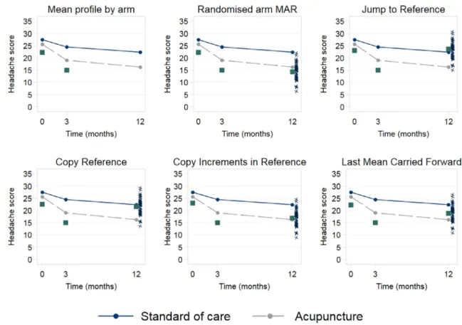
• In a two arm trial of an active versus a reference treatment, we could impute missing data assuming patients jump to behave like those in a specified reference arm following their last observed time point. This may be suitable when any treatment effect would be expected to stop following drop out. This has been termedjump to referenceimputation. For example, in the acupuncture versus standard care headache trial, we could impute missing data assuming patients jump to follow the behavior of the standard care arm following their last observed time point. This scenario, consid-ered the most plausible sensitivity analysis for the headache trial, is illustrated schematically in the top right panel of Figure 4.
F I G U R E 4 Example reference based imputation models for the acupuncture trial. The squares at time 0 and 3 are observed values for a participant in the acupuncture arm who withdrew after the 3 month visit. The black arrows represent the imputation distributions. The squares at time 12 are the mean of the imputed values for that participant in the given reference based scenario. The crosses at time 12 represent the individual imputed values around that mean across 50 multiply imputed datasets for the withdrawing active participant. The reference arm is the standard care arm. This is not an exhaustive display of the MNAR options possible within the reference-based framework [Colour figure can be viewed at wileyonlinelibrary.com]
• Alternatively, we could impute assuming patient outcomes follow the mean increments observed in a reference arm following their last observed time point. This is referred to ascopy increments in reference(CIR) imputation. Within the acupuncture arm, we could impute assuming the differences in patients mean outcomes over time follow those observed in the standard care arm (bottom row center panel of Figure 4).
• A third option is to impute assuming patients behaved as if they were in a specified reference arm for the full duration of the trial, known ascopy reference(CR) imputation. In the acupuncture trial, we could impute assuming patients followed the standard care arm behavior for the full trial duration (bottom row left panel of Figure 4), a natural option when we believe patients followed a different (reference) treatment from their randomized allocation throughout the trial.
• Alternatively,last mean carried forward(LMCF) imputes assuming patient behavior stays at the mean level for their randomized arm at their last observed time point, appropriate when we believe the effect of randomized treatment is maintained on average over time. This is a more principled version of the classic LOCF analysis (bottom right row panel, Figure 4).
Table 2 summarizes these five imputation options proposed by Carpenter et al11for a continuous outcome. The options
in Table 2 are not an exhaustive listing of reference based options. Naturally under any reference based method discussed above, for patients in the designated reference arm, their data will be imputed as under randomized arm MAR. Using data from the acupuncture headache trial, we will demonstrate how reference based MI can be accessibly conducted in Stata using themimixcommand under these five assumptions.45Further technical details on the underlying reference
based algorithm are provided in Appendix B.
We will first conduct primary analysis under the most plausible randomized-arm MAR assumption for the unobserved data using the reference based MI algorithm of Carpenter et al.11Themimixcommand can be downloaded within Stata
T A B L E 2 Examples of reference based multiple imputation options
Method Description
Randomized-arm MAR Impute assuming patients follow the behavior of their randomized arm. The joint distribution of patients' pre- and post-deviation outcome data is MVN with mean and covariance matrix from their randomized arm.
Jump to reference (J2R) Impute assuming patient behavior jumps to that of a specified reference arm. The joint distribution is MVN with mean vector from the patients randomized arm up to their last observation time, post-deviation the mean vector follows that observed for a reference group (typically control). The covariance matches the randomized arm for pre-deviation measurements and the reference arm for the conditional components of post- given pre-deviation measurements.
Last mean carried forward (LMCF) Impute assuming patient behavior remains at the mean level for their randomized arm at their last observed time point. The joint distribution is MVN with mean vector from the patients randomized arm up to their last observation time, post-deviation the means are set equal to the marginal mean for the patients randomized arm at their last observed time. The covariance matrix remains as that for their randomized treatment arm.
Copy increments in reference (CIR) Impute assuming patient behavior follows the mean increments observed in a specified reference arm. The joint distribution is MVN with mean vector from the patients randomized arm up to their last observed time, post-deviation the patients mean increments follow those from a reference arm. The covariance is the same as in J2R. Appropriate when we wish to assume that post-deviation the disease resumes the course observed in the reference arm.
Copy reference (CR) Impute assuming patients follow the behavior of a specified reference arm for the duration of the trial. The joint distribution of patients' pre- and post-deviation outcome data is MVN with mean and covariance matrix from a reference arm regardless of deviation time.
by typingssc install mimix. A detailed specification of the commands options is available in Cro et al.45A freely
available SAS macro by Roger46calledmiwithdalso implements the algorithm of Carpenter et al. The “five-macros”
SAS package, which is a more developed version of themiwithdmacro, is also available for analysis within SAS.47Both
SAS implementations are available for download at www.missingdata.org.uk.
Within the headache dataset,idis the unique individual identifier andtreatis the randomized treatment assign-ment to standard care (treat = 0) or acupuncture (treat = 1). Baseline covariates include the randomization stratification factors ofage,sex,migrane(diagnosis of migraine or tension-type), andchronicity(number of years of headache disorder).head_baseis the baseline headache score.headis the post-baseline headache score andtimeis the time of the headache measurement in months (3 or 12 months). The dataset is in “long” format, with one observation per individual per time point, asmimixrequires.
We impute under MAR and create 50 imputations using an MCMC burn-in of 1000 and burn-between of 500 iterations as recommended by Carpenter and Kenward (p. 84).5We include the randomization stratification factors ofage,sex,
migrane, andchronicityin the imputation model. The baseline headache measure (head_base) is also included in the imputation model as a covariate, but if this fully observed variable were used as an outcome in the imputation model, the imputation results would be stochastically identical. We includehead_baseas a covariate here so that it will be treated as a covariate in the analysis step; we use theregressoption to specify that the substantive analysis is a linear regression of 12-month headache score (final time point) on randomized treatment and the included covaraites (age, sex,migrane,chronicity, andhead_base). Theregressoption fits a linear regression of the outcome at the final time point on treatment arm and any covariates included in the imputation model post MI to each imputed dataset, then combines results using Rubins' rules. If an alternative substantive model of interest were required, theregressoption is not required and the imputed datasets can instead be saved for use with a different analysis model. Although possible, we caution against the use of an analysis model that has variables or structure (eg, interaction terms) not included in the imputation process because this will create additional imputation-analysis model incompatibility. As discussed in Section 3.4, when performing MI under MAR, it is important that the imputation model includes (at a minimum) all
T A B L E 3 Sensitivity analysis results for the headache trial using reference based MI withK=50 imputations
Analysis Treatment Est. (L) 95% CI SE P-value
Primary analysis
Randomized-arm MAR −4.97 −7.40 to−2.54 1.23 <0.001
Sensitivity analysisa
Jump to standard care −3.32 −5.70 to−0.94 1.21 0.006
Copy increments in standard care −3.74 −6.07 to−1.41 1.18 0.002
Copy standard care −3.80 −6.12 to−1.49 1.18 0.001
Jump to acupuncture −3.00 −5.44 to−0.56 1.24 0.016
Copy increments in acupuncture −3.50 −5.91 to−1.10 1.22 0.004
Copy acupuncture −3.48 −5.87 to−1.09 1.21 0.005
Last mean carried forward −4.94 −7.38 to−2.50 1.24 <0.001
aSensitivity analysis results are sorted in terms of what we considered the most plausible assumption (higher position vertically)
to least plausible assumption (lower position vertically).
the variables to be included in the analysis model to ensure unbiased estimation. Although the imputation and analysis model will not in fact be fully compatible in reference based settings, the implications of which we expand further on in Section 6, the imputation model should include all variables to be included in the analysis. Thesavingoption specifies that the imputed datasets will be saved in a Stata data file calledhead_mar. The commands required are as follows.
⋅ use acupuncture, clear
⋅ mimix head treat, id(id) time(time) covariates(age sex migraine chronicity
head_base) method(mar) m(50) regress clear seed(23) burnin(1000) burnbetween(500) saving(head_mar)
For sensitivity analysis, to impute under the next mot plausible assumption J2R, where the reference group is the standard care arm, we update the method specification to “j2r” and add that treatment=0 (standard care) is the reference group, using therefgroupoption, as follows:
⋅ mimix head treat, id(id) time(time) covariates(age sex migraine chronicity head_base) method(j2r) refgroup(0) m(50) regress clear seed(23) burnin(1000) burnbetween(500) saving(head_j2r0)
To impute under J2R where the reference arm is the acupuncture arm, we use the above code but alternatively indicate that refgroup=1. To impute under CIR, CR, or LMCF, the above line of code is adapted to includecir,cr, orlmcfin place ofj2r, with the required reference group (or no reference group in the case of LMCF).
The primary MAR analysis (Table 3) suggests that acupuncture results in improved headache scores relative to stan-dard care, with a treatment effect of−4.97. Sensitivity analysis results are sorted by plausibility (what we considered most plausible, down to what we considered least plausible). After MAR, we considered it most plausible that patients in the acupuncture arm discontinued treatment abruptly following their last observed outcome measurement and then jumped to follow the behavior observed in the standard care arm; unobserved outcomes of individuals in the stan-dard care arm assumed to be MAR. Under jump to stanstan-dard care, the treatment effect is lower at−3.32. Assuming that patients in the acupuncture arm more gradually tracked toward the standard care arm behavior following with-drawal, copy increments in standard care