Object Classification and Detection
in High Dimensional Feature Space
THIS IS A TEMPORARY TITLE PAGE It will be replaced for the final print by a version
provided by the service académique.
Thèse n. 6043
présentée le 17 Décembre 2013
à la Faculté Sciences et Techniques de l’Ingénieur Laboratoire de l’Idiap
Programme doctoral en Informatique, Communications et Infor-mation
École Polytechnique Fédérale de Lausanne pour l’obtention du grade de Docteur ès Sciences par
Charles Dubout
acceptée sur proposition du jury: Prof Mark Pauly, président du jury Dr François Fleuret, directeur de thèse Prof Pascal Fua, rapporteur
Prof Gilles Blanchard, rapporteur Prof Frédéric Jurie, rapporteur Lausanne, EPFL, 2013
Acknowledgements
First and foremost, I would like to thank my thesis advisor, Dr. François Fleuret, for giving me the opportunity to carry out this very exciting project. François has all the qualities a PhD student can dream of: he is always there when you need him, ready to discuss new ideas, he has a deep knowledge not only of the field but also of CS and math in general, and he never urges you but instead gives you all the freedom you might need to carry out your work to fruition. He also taught me what it means to be a real scientist, in addition of an engineer, which I always wanted to be.
I would like also to thank my three jury members, Prof. Pascal Fua, Prof. Gilles Blanchard, and Prof. Frédéric Jurie, as well as my jury president, Prof. Mark Pauly, for doing me the honor to supervise my oral exam.
Many thanks to Dr. Raghuraman Krishnamoorthi, Dr. Bojan Vrcelj, and all their colleagues for giving me the opportunity to come to the U.S. and mentoring me during my internship at Qualcomm San Diego. Experiencing life in California and working in a large IT company was very interesting and something I always wanted to try.
Working at Idiap would not have been as fun without all my office mates and colleagues: Adolfo, Alexandre2, Alexandros, André, Arjan, Ashtosh, Barbara, Bastien, Cheng, Chidansh, Chris, Cosmin, Daira, David, Elie, Flavio, Francesco, Gulcan, Gwénolé, Hugo, Hui, Ilja, Ivana, Jagan, James, Jean-Marc, Joan, Joel, Kenneth, Laurent2, Leo, Majid, Manuel, Marc, Marco, Maryam, Mathew, Minh-Tri, Nadine, Nesli, Nicolae, Nik, Nikolaos, Novi, Olivier, Oya, Paco, Paul, Philip2, Pierre-Edouard, Radu, Raphaël, Riwal, Roger, Romain, Ronan, Roy, Rui, Rémi2, Samira, Serena, Sylvie, Tatiana, Teodora, Thomas, Valérie, Vincent, Yann and probably a few others which I forgot, sorry! I will not soon forget all the long baby foot games we played, all the Friday afternoon beers, and all our (sometimes a bit pointless, Boosting vs. SVM anyone?) discussions.
I would finally like to thank my parents, in-laws, brothers and sisters, and all the rest of my family for their constant support. Special thanks to my wife Wenqi, always there to share with me the highs and lows of PhD life and without who none of it would have been possible. Charles Dubout was supported by the Swiss National Science Foundation under grant 200021-124822 – VELASH.
Lausanne, 20 December 2013 Charles
Abstract
Object classification and detection aim at recognizing and localizing objects in real-world images. They are fundamental computer vision problems and a prerequisite for full scene understanding. Their difficulty lies in the large number of possible object positions and the appearance variations of object classes. This thesis improves upon several classical machine learning algorithms, enabling large computational gains in high dimensional feature space. A common trend in machine learning and computer vision research is to go large scale. In particular, the advent of huge datasets mined from the Internet, and the combination of multiple feature sources have considerably broadened the applications of computer vision. Tasks which were thought impossible a few years ago, such as human action recognition or pose estimation, automatic outdoor navigation,etc., now seem within reach.
This dissertation is divided into two parts. The first one deals with the efficient training of a classifier or detector based on a large number of feature extractors, outside the control of the learning algorithm, and therefore of unknown suitability to the task at hand. More precisely, this part presents two kinds of strategies to accelerate the training of Boosting algorithms in such a context: (a) a method to better deal with the increasingly common case where features come from multiple sources (e.g.color, shape, texture,etc., in the case of images) and therefore can be partitioned into meaningful subsets; (b) new algorithms which balance at every Boosting iteration the number of weak learners and the number of training examples to look at in order to maximize the expected loss reduction. Experiments in image classification and object recognition on four standard computer vision datasets show that the adaptive techniques we propose outperform both basic sampling and state-of-the-art bandit methods. The second part deals with linear object detectors, currently the most popular class of detec-tion systems, encompassing template matching, deformable part models, poselets, convolu-tional neural networks (which internally use linear filters),etc.The main bottleneck of many of those systems is the computational cost of the convolutions between the multiple rescalings of the image to process and the linear filters. We make use of properties of the Fourier transform and clever implementation strategies to obtain a speedup factor proportional to the filter size, both while training and at test time. We also introduce a few modifications to the original Deformable Part Model (DPM) of Felzenszwalbet al.improving its detection accuracy. The gains in performance are demonstrated on the well-known Pascal VOC benchmark, where an increase by one order of magnitude in the speed of said convolutions, and an average improvement of 15% in the accuracy of the detector are established.
Keywords:Boosting, large scale learning, feature selection, linear object detection, deformable part model
Résumé
La classification et la détection d’objets visent à reconnaître et à localiser des objets dans des images du monde réel. Ce sont des problèmes fondamentaux de vision par ordinateur qui constituent un prérequis à la compréhension de scènes complètes. Leur difficulté vient du large nombre de positions potentielles et de la diversité d’apparence propres à chaque classe d’objets. Cette thèse présente plusieurs améliorations d’algorithmes classiques d’ap-prentissage automatique, diminuant grandement leur coût computationnel en espaces de caractéristiques de grandes dimensions.
Une des tendances actuelles de la recherche en apprentissage automatique et en vision par ordinateur est de considérer des échelles toujours plus grandes. En particulier, l’avènement d’énormes ensembles de données compilés à partir d’Internet, et la combinaison de plusieurs sources de caractéristiques visuelles ont considérablement étendu les champs d’application de la vision par ordinateur. Des tâches qui semblaient impossible il y a quelques années, telles que la reconnaissance de l’activité ou de la pose d’êtres humains, la navigation automatique en extérieurs,etc., semblent maintenant proches d’être réalisables.
Cette dissertation est divisée en deux parties. La première traite de l’entraînement efficace d’un classificateur ou d’un détecteur basé sur un grand nombre d’extracteurs de caractéristiques visuelles, hors du contrôle de l’algorithme d’apprentissage, et dont la pertinence vis-à-vis de la tâche à résoudre est inconnue. Plus précisément, cette première partie présente deux types de stratégies visant à accélérer l’entraînement d’algorithmes de Boosting dans ce contexte : (a) une méthode pour gérer le cas de plus en plus courant où les caractéristiques sont issues de plusieurs sources (ex.couleur, forme, texture,etc., dans le cas d’images) et peuvent donc être partitionnées en sous-ensembles de façon non-arbitraire ; (b) de nouveaux algorithmes qui équilibrent à chaque itération de Boosting le nombre de classifieurs faibles et le nombre d’exemples d’apprentissage dans le but de maximiser l’espérance de la réduction de la fonction de coût. Quatre expériences en classification d’images et en reconnaissance d’objets sur des ensembles de données standards montrent que les techniques adaptatives que nous proposons surpassent des techniques d’échantillonnage basiques ainsi que des méthodes de pointe utilisant des bandits manchots.
La seconde partie traite de détecteurs d’objets linéaires, actuellement la classe de détecteurs la plus populaire, incluant la comparaison avec des motifs standards, les modèles à parties déformables, les poselets, les réseaux de neurones à convolution (qui utilisent des filtres linéaires en interne),etc.Le principal goulot d’étranglement de la plupart de ces systèmes est
le coût computationnel des convolutions entre les multiples redimensionnements de l’image à traiter et des filtres linéaires. En utilisant certaines propriétés de la transformée de Fourier ainsi que d’ingénieuses stratégies d’implémentation, nous obtenons un gain d’accélération proportionnel à la taille des filtres, à la fois durant l’entraînement et durant le test. Nous présentons aussi quelques modifications apportées au modèle à parties déformables originel de Felzenszwalbet al.améliorant sa précision en détection. Les gains apportés en performance sont démontrés sur le célèbre Pascal VOC benchmark. Une accélération de la vitesse des convolutions d’un ordre de grandeur, ainsi qu’une amélioration moyenne de la précision du détecteur de 15% sont démontrées.
Mots-clés :Boosting, apprentissage à grande échelle, sélection de caractéristiques, détection d’objet linéaire, modèle à parties déformables
Contents
Acknowledgements iii
Abstract (English/Français/Deutsch) v
List of figures xi
List of algorithms xiv
List of tables xv
1 Introduction 1
1.1 Learning in High Dimensional Feature Space: Advantages and Challenges . . . 1
1.2 Organization and Contribution of this Thesis . . . 3
1.3 Notation . . . 5
Part I: Boosting in High Dimensional Feature Space 7 2 Influence of the number of Training Examples and Features on Boosting 9 2.1 Introduction and related works . . . 11
2.1.1 AdaBoost . . . 11
2.2 Experiments . . . 13
2.3 Conclusion . . . 19
3 Adaptive Sampling for Large Scale Boosting 21 3.1 Introduction . . . 23 3.2 Related works . . . 23 3.3 Preliminaries . . . 25 3.3.1 Standard Boosting . . . 25 3.3.2 Feature subsets . . . 26 3.4 Tasting . . . 26 3.4.1 Main algorithm . . . 26 3.4.2 Tasting variants . . . 27
3.4.3 Relation with Bandit methods . . . 28
3.5 Maximum Adaptive Sampling and Laminating . . . 29
3.5.2 Modeling the true edge . . . 30 3.5.3 M.A.S. variants . . . 31 3.5.4 Laminating . . . 32 3.6 Experiments . . . 35 3.6.1 Features . . . 35 3.6.2 Datasets . . . 35
3.6.3 Uniform sampling baselines . . . 36
3.6.4 Bandit sampling baselines . . . 37
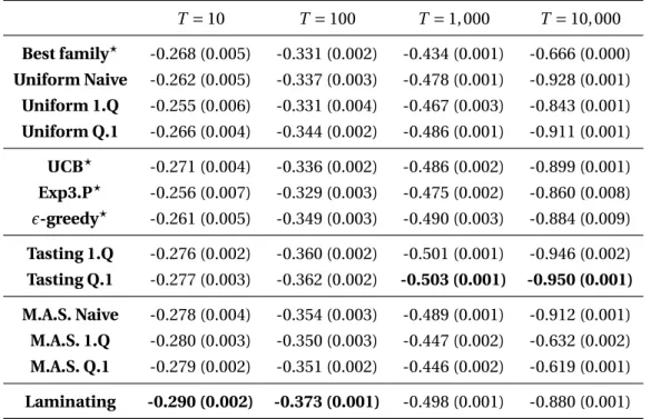
3.6.5 Results . . . 38
3.7 Conclusion . . . 39
Part II: Object Detection in High Dimensional Feature Space 53 4 Accelerated Evaluation of Linear Object Detectors 55 4.1 Introduction . . . 57
4.2 Related works . . . 57
4.3 Linear object detectors and Fourier transform . . . 58
4.3.1 Evaluation of a linear detector as a convolution . . . 59
4.3.2 Leveraging the Fourier transform . . . 60
4.4 Implementation strategies . . . 62
4.4.1 Patchworks of pyramid scales . . . 62
4.4.2 Taking advantage of the cache . . . 63
4.5 Experiments . . . 66
4.6 Conclusion . . . 67
5 Accelerated Training of Linear Object Detectors 69 5.1 Introduction and related Works . . . 71
5.2 Evaluation of the gradient of a linear detector as a convolution . . . 71
5.3 Computational cost of the gradient computation . . . 73
5.4 Experiments . . . 74
5.4.1 Implementation details . . . 75
5.4.2 Results . . . 76
5.5 Conclusion . . . 78
6 Extensions to the original Deformable Part Model 79 6.1 Introduction . . . 81
6.2 Related works . . . 81
6.3 Standard Deformable Part Models . . . 82
6.4 Additional features . . . 84
6.4.1 Histograms of uniform Local Binary Patterns . . . 84
6.4.2 Color histograms . . . 85
6.4.3 Experiments . . . 86
Contents
6.5.1 Extension to 3D . . . 88
6.5.2 Approximation to the generalized distance transform . . . 88
6.5.3 Experiments . . . 90
6.5.4 Results . . . 92
6.6 Joint appearance constraints . . . 93
6.6.1 Post-scoring (DPM†) . . . 94
6.6.2 Joint-scoring (DPM‡) . . . 94
6.6.3 Learning . . . 94
6.6.4 Experiments . . . 95
6.7 Conclusion . . . 95
7 Summary and Future Directions 97 7.1 Discussion . . . 97 7.2 Future Directions . . . 98 A Proof of Lemma 1 99 B Proof of Theorem 1 101 Bibliography 108 Curriculum Vitae 109
List of Figures
1.1 Influence of the number of training examples and features on SVRT. . . 3
2.1 Exponential loss . . . 12
2.1 The 23 visual categorization problems. . . 15
2.2 Results of AdaBoost on the 23 visual categorization problems. . . 18
3.1 Simulation of the expectation of²∗in the Gaussian case . . . 30
3.2 Difference between the maximum edge and the best edge for Laminating . . . 34
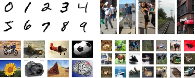
3.3 Example images from the four datasets used in the experiments . . . 36
3.4 Mean Boosting loss on the MNIST dataset. . . 44
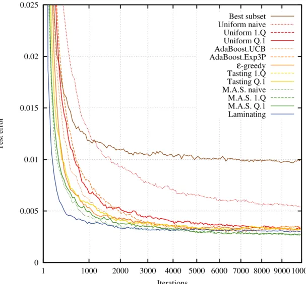
3.5 Mean test error on the MNIST dataset. . . 45
3.6 Mean Boosting loss on the INRIA Person dataset. . . 46
3.7 Mean test error on the INRIA Person dataset. . . 47
3.8 Mean Boosting loss on the Caltech 101 dataset. . . 48
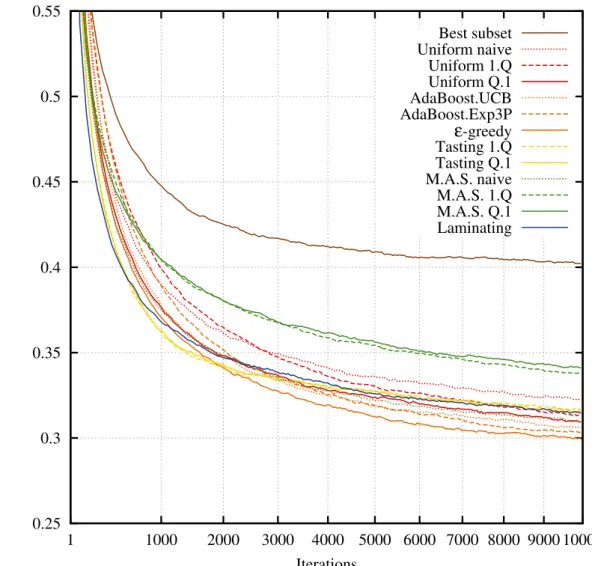
3.9 Mean test error on the Caltech 101 dataset. . . 49
3.10 Mean Boosting loss on the CIFAR-10 dataset. . . 50
3.11 Mean test error on the CIFAR-10 dataset. . . 51
4.1 Histogram of Oriented Gradients . . . 58
4.2 HOG feature planes . . . 59
4.3 Standard convolution process . . . 60
4.4 Fast Fourier convolution process . . . 61
4.5 Patchwork of images . . . 62
4.6 Fragment strategy . . . 64
4.7 Fragment size . . . 65
5.1 Computation of the gradient of the loss . . . 72
5.2 Root filters for a bicycle model of normal size . . . 76
5.3 Root filters for a bicycle model of double the normal size . . . 76
6.1 Examples of detections on the Pascal VOC challenge 2007. . . 82
6.2 Standard Standard Deformable Part Model. . . 83
6.3 Local Binary Pattern operator using a 3×3 neighborhood. . . 84
6.5 Color histograms . . . 86 6.6 Examples of detections on the Pascal VOC challenge 2007 using a 3D model. . . 88 6.7 Deformation across scales . . . 89 6.8 Root and part locations in 2D and 3D. . . 90
List of Algorithms
2.1 AdaBoost, the most common Boosting algorithm. . . 13
3.1 Tasting 1.Q . . . 27
3.2 Tasting Q.1 . . . 28
3.3 M.A.S. . . 32
3.4 Laminating . . . 33
4.1 Fast Fourier convolution process . . . 66
List of Tables
1.1 Single feature versus feature combination methods comparison. . . 2
2.1 Mean results of AdaBoost on the 23 visual categorization problems. . . 18
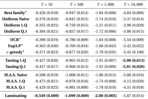
3.1 Mean Boosting loss on MNIST . . . 40
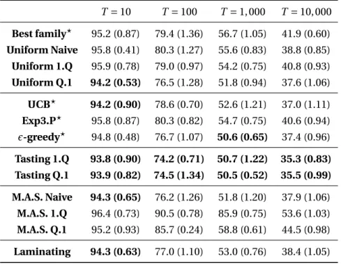
3.2 Mean test error on MNIST . . . 40
3.3 Mean Boosting loss on INRIA Person . . . 41
3.4 Mean test error on INRIA Person . . . 41
3.5 Mean Boosting loss on Caltech 101 . . . 42
3.6 Mean test error on Caltech 101 . . . 42
3.7 Mean Boosting loss on CIFAR 10 . . . 43
3.8 Mean test error on CIFAR 10 . . . 43
4.1 Asymptotic memory footprint and computational cost for the three approaches described in § 4.4.1 . . . 63
4.2 Pascal VOC 2007 challenge results. . . 67
4.3 Pascal VOC 2007 challenge convolution time and speedup. . . 68
5.1 Performance of our trained mixture on Pascal VOC 2007 . . . 77
5.2 Average time to compute the gradient of the loss . . . 77
6.1 Performance of models using additional features on Pascal VOC 2007 . . . 87
6.2 Performance of the 2D and 3D models on Pascal VOC 2007 . . . 91
1
Introduction
This introduction presents an overview of learning in high dimensional feature space (§ 1.1) and the contribution of this thesis (§ 1.2). The motivations presented here are elaborated further in the following chapters. At the end of this chapter, we also introduce the notation and the necessary mathematical tools used in this thesis § 1.3.
1.1 Learning in High Dimensional Feature Space: Advantages and
Challenges
A common trend in machine learning and computer vision research is to go “large scale”, both in the number of training examples (e.g.ImageNet (Deng et al., 2009) contains currently close to ten million images, i.e. approximately ten terabyte of raw data) and the number of features considered (e.g.shape, color, texture,etc.). Such increase in the size of datasets and the number of features, together with the advent of more sophisticated learning algorithms led to major improvement in classification performance and in the range of problems which can now be tackled (action recognition, pose estimation, automatic outdoor navigation,etc.). In particular using more features can improve performance by increasing the amount of information given to the learning system, make the system more robust, and can even make the problem simpler by making it more separable. Two practical examples are displayed in table 1.1 and in figure 1.1. The first example, adapted from (Gehler and Nowozin, 2009), reports the test accuracy of various kernel methods trained either on a single or on a combination of all the seven features used by the authors in their experiments. The main observation they made is that the learning method often does not matter much, all of the algorithms performing similarly in that particular experiment, but that using a combination of features can be crucial in order to get the best out of a classifier. The second example, adapted from (Fleuret et al., 2011), plots the test error of an AdaBoost classifier on the Synthetic Visual Reasoning Test (SVRT) for various number of training examples and groups of features. SVRT is a series of 23 image classification problems, each containing images of simple shapes, positive or negative according to some high-level rule, typically easy to understand for humans but hard for
off-Table 1.1 – Mean classification accuracy on the Oxford Flowers dataset (Nilsback and Zisser-man, 2006) of several classification methods using either a single features or a combination of all of them. The learning method does not matter much, combining features is much more important. Reprinted from (Gehler and Nowozin, 2009).
Single feature Combination methods
Method Accuracy Time Method Accuracy Time
Color 60.9±2.1 3 product 85.5±1.2 2 Shape 70.2±1.3 4 averaging 84.9±1.9 10 Texture 63.7±2.7 3 CG-Boost 84.8±2.2 1225 HOG 58.5±4.5 4 MKL (SILP) 85.2±1.5 97 HSV 61.3±0.7 3 MKL (Simple) 85.2±1.5 152 siftint 70.6±1.6 4 LP-β 85.5±3.0 80 siftbdy 59.4±3.3 5 LP-B 85.4±2.4 98
the-shelf machine learning algorithms. The features from group 1 only count pixels in boxes, those of group 2 also look at edges, and the ones in group 3 also look at properties of the whole image (Fourier and wavelet coefficients). The performance of the classifier increases with both, overfitting decreasing with the number of training examples, while the more complex features make some tasks much easier to solve. For example tasks which necessitate to match shapes become easier with features from group 2, while tasks necessitating to look at the whole image (for example to detect alignment or symmetry) become much easier with the ones from group 3. A more in-depth analysis of SVRT and these results is the topic of chapter 2. But this trend towards larger and larger datasets also poses deep scalability issues, since it might become difficult to store and process all this information. For instance it might be impossible for an object detector to extract and store all patches from all training images of a large dataset on current hardware.
Current feature combination techniques such as classifier or feature concatenation, multiple kernel learning (MKL) (Lanckriet et al., 2004; Bach et al., 2004) or LP-β(Gehler and Nowozin, 2009) pay little attention to their computational cost, and assume that all the features have been selected by an expert, meaning that they do not expect most features to be irrelevant. Even when considering a single kind of feature, as is often the case in object detection, the amount of data that has to be processed is often huge due to the sheer number of overlapping image sub-windows, so that even ‘fast’ linear methods can struggle.
Our aim is therefore to address the following research questions:
• How to train a classifier efficiently using multiple kind of uncontrolled features, of various usefulness?
1.2. Organization and Contribution of this Thesis
0 0.25 0.5
10 100 1000 10000
Test error rate
Number of examples
(a) Influence of the number of examples.
0 0.25 0.5
1 2 3
Test error rate
Feature groups
(b) Influence of the number of features.
Figure 1.1 – Influence of the number of training examples and the amount/complexity of the features on the Synthetic Visual Reasoning Test (SVRT). The features from group 1 only count pixels in boxes, those of group 2 also look at edges, and the ones in group 3 look at properties of the whole image (Fourier and wavelet coefficients). Reprinted from (Fleuret et al., 2011).
• How to make large scale learning faster (large in the number of examples and features)? • Is it possible to speed up object detection over dense features by exploiting the overlap
between samples?
• How to best exploit this speed up to improve detection accuracy?
We propose to consider the first two questions in the Boosting framework. We believe Boosting to be well suited for this task due to its iterative building process, enabling it to do feature selection while training. Each training iteration can be restricted to look only at a small subset of examples and features, limiting the total computational cost, instead of looking at everything all the time, as would be the case with support vector machines (Vapnik, 1995) or classical neural networks. Its linear nature also makes it easy to understand the contribution of each feature, and to prune away useless ones.
For the last two questions we turned to linear classifiers, which have been hugely popular in recent years in the vision community. We focus particularly on the Deformable Part Model (DPM) of Felzenszwalbet al.(Felzenszwalb et al., 2010b), which has received the most attention in recent years, but our analyses remain applicable to a wider range of object detectors.
1.2 Organization and Contribution of this Thesis
This thesis is organized in two parts. After defining Boosting and stressing out the importance of large scale learning in chapter 2, using SVRT as an illustration, chapter 3 describes three new families of algorithms to improve Boosting in high dimensional feature space, particularly when dealing with multiple kind of features and a large number of examples.
The first one, Tasting, is a strategy to bias feature sampling towards promising subsets. Con-trarily to previously existing methods (LazyBoosting (Escudero et al., 2000), AdaBoost.UCB (Busa-Fekete and Kegl, 2009) and its later variants (Busa-Fekete and Kegl, 2010),etc.), it con-tinuously estimates the expected quality of each feature subset from a limited set of features sampled prior to the learning, as well as the current Boosting weights. As for the bandit-related methods which we use as baselines, Tasting exploits the fact that the full feature set is a hetero-geneous union of somehow homohetero-geneous subsets of features. It exploits the main strength of Boosting which is to spot and combine complementary features, and can thus discard features redundant with features already chosen.
The second one, Maximum Adaptive Sampling (abbreviated M.A.S.) is a family of algorithms targeted at learning in high dimensional feature space with or without multiple feature subsets. They model at every Boosting step the distribution of the performance of the weak learners, and computes from it the optimal number of examples and weak learners to sample under a given cost constraint.
The third one, Laminating, tries to reduce the requirement for a density model of the weak learners’ performance. At every Boosting step it iteratively halves the number of considered weak learners, and doubles the number of samples, until only one weak learner remains. The second part proposes acceleration strategies applicable to a wide class of linear object detector. It focuses particularly on the currently state-of-the-art linear object detector of Felzenszwalbet al.(Felzenszwalb et al., 2010b), and describes improvement to its efficiency and its detection accuracy.
Current state-of-the-art linear object detection methods compute the convolutions between image features and trained linear filters directly, with a cost proportional to the size of the linear filters. They work by first extracting features from the input images, often at multiple resolutions. Those image and filter features can be seen as being organized in planes, each containing a distinct feature at the same image locations. Existing methods compute the convolution of an image feature planes and a linear filter by first convolving each feature plane independently, and summing the results together. The novelty of our invention exposed in chapter 4 is to do the convolution using a Fast Fourier Transform (FFT) algorithm and to take advantage of the linearity of the transform to reduce the number of required inverse transforms to one per filter at detection time (instead of the number of features). We also came up with two additional implementations strategies, both necessary in order to get the most out of the method, and obtain one order of magnitude speedup compared to previous implementations.
In chapter 5 we rewrite the computation of the gradient of the loss minimized during training as a convolution. This enables us to accelerate training as well for any loss written as a sum over the examples, making the overall training computational cost independent of the filters’ sizes. It relieves all the constraints inherent to sparse and approximate methods, but is not always as efficient, as we experimentally observed.
1.3. Notation
Chapter 6 presents three extensions to the original DPM of Felzenszwalbet al.The first one is to use different kinds of features in addition to HOG. We settled for histograms of Local Binary Patterns (LBP), a widely used texture descriptors, and our own color histograms. These are similar to HOG in that they are local histograms computed over the pixels of each cell of a dense grid, but instead of being histograms of the gradient orientation weighted by the gradient magnitude, they are respectively histograms of the LBP binary code or the hue weighted by the saturation.
The second one removes a limitation of current DPMs, in which parts deform only at a fixed predetermined scale relative to that of the root of the models (typically at twice the resolution). They do so because it enables them to find the optimal placement of each part efficiently, using a fast 2D distance transform algorithm. By settling for approximately optimal placements, we were able to efficiently deform the parts across scales as well, by reusing the original convolutions and distance transforms. Allowing parts to move in 3D increases the expressivity of the models, and might approximate an increase in the scanning resolution.
The third extension addresses a shortcoming of the standard DPM: its complete ignorance of joint aspects of appearance, marginalizing it completely over the parts. We therefore proposes to add to the model a term looking jointly at the appearance of the part and the root together, which has the advantage compared to other joint models to be simpler and more efficient.
1.3 Notation
In this section we introduce formally the notations as well as the necessary mathematical tools used in this thesis.
Notation.We indicate scalars with lower case letters (e.g. xandλ), vectors and matrices with bold letters (e.g.xandw), and sets with calligraphic font (e.g.X andH). In order to make index expressions more readable, we usex(i,j) rather thanxi jto refer to the element in the
ithrow and thejthcolumn of matrixx. Thusxk(i,j) signifies the element of indicesiandjin xk, the matrix of indexk. The set of real numbers is denoted byRand the indicator function,
Boosting in High Dimensional Feature
Space
2
Influence of the number of Training
Examples and Features on Boosting
In this chapter we present our observations on the influence of the number of training examples and features on the classification performance of AdaBoost, the most popular Boosting algo-rithm. The dataset that we used is the Synthetic Visual Reasoning Test (SVRT), a collection of twenty-three synthetic image classification problems. While only a few images are necessary for humans to grasp the rule underlying each problem, general machine learning methods often require thousands of examples as well as elaborate image features to achieve their optimal performance. Content presented in this chapter is based on the following publications (Fleuret et al., 2011):F. Fleuret., T. Li, C. Dubout, E. K. Wampler, S. Yantis, and D. Geman. Comparing machines and humans on a visual categorization test. InProceedings of the National Academy of Sciences, 2011.
2.1. Introduction and related works
2.1 Introduction and related works
Boosting is a powerful approach to improve the performance of a given “weak” learning algorithm (i.e.one that performs just slightly better than random guessing) by combining them into a “strong” learning algorithm. While Boosting is not algorithmically constrained, most Boosting algorithms work by iteratively training the same weak classifier with a different weighting over the training examples. At each iteration, the weighting distribution gives em-phasis to the “hardest” (most incorrectly classified) examples. The final “strong” classifier is obtained as an average of the trained weak learners, weighted by some function of their re-spective accuracy. Under some mild assumptions, and given a sufficient number of iterations, the training error of the final combination can become arbitrarily low (Schapire et al., 1998). It has also been repeatedly observed in practice that Boosting is relatively immune to overfitting, as the testing error typically continues to decrease long after the training error reaches zero.
2.1.1 AdaBoost
In this thesis we will focus on the (discrete) AdaBoost (short for Adaptive Boosting) algorithm, by far the most popular and extensively studied Boosting algorithm (Friedman et al., 2000). We concentrate on the binary classification task and let the training set be
(xn,yn)∈X×{−1, 1},n=1, . . . ,N. (2.1)
The goal is to construct a strong classifier of the form
F(x)=sign¡ f(x)¢ (2.2) with f(x)= T X t=1 αtht(x) (2.3)
whereht(x) denotes a binary weak learner,i.e.a function of the formX→{−1, 1} andαt∈R
denotes its weight.
Given a set of weak learners H, the choice ofht ∈H at each iteration results from the
minimization of the Exponential loss
L(f)= N X n=1 exp¡−ynf(xn) ¢ . (2.4)
This cost function penalizes samples that are wrongly classified (ynf(xn)≤0) much more
heavily than those that are classified correctly (ynf(xn)>0). It upper-bounds the Hamming
loss, which in the binary case is equivalent to the training error (see figure 2.1). Directly optimizing (2.4) is complex and AdaBoost employs instead a greedy approach, optimizing each pair ofαt,htiteratively (see algorithm 2.1).
ynf(xn) l oss −1.5 −1 −0.5 0 0.5 1 1.5 0 1 2 3 4 5 Exponential: exp¡ −ynf(xn)¢ Hamming:1{ynf(xn)≤0}
Figure 2.1 – An illustration of how the Exponential loss (in red) upper-bounds the Hamming loss (in blue), directly related to the training error since1{F(xn)6=yn}=1{ynf(xn)≤0}.
Suppose thattpairs ofαt,hthave already been optimized, and let
ft= t X i=1
αihi. (2.5)
stands for the current classifier. The next pair picked by AdaBoost is (αt+1,ht+1)= argmin (α∈R,h∈H) L(ft+αh) (2.6) = argmin (α∈R,h∈H) N X n=1 exp¡−yn ¡ ft(xn)+αh(xn) ¢¢ (2.7) = argmin (α∈R,h∈H) N X n=1 exp¡−ynft(xn) ¢ exp¡−ynαh(xn) ¢ . (2.8) If we define ωt(n)= exp¡ −ynft(xn)¢ PN i=1exp ¡ −yift(xi)¢ =exp ¡ −ynft(xn)¢ L(ft) (2.9)
the normalized weight associated with examplen, we can rewrite (2.8) as
(αt+1,ht+1)= argmin (α∈R,h∈H) N X n=1 ωt(n) exp¡−ynαh(xn)¢. (2.10)
2.2. Experiments
Algorithm 2.1AdaBoost, the most common Boosting algorithm.
Input: (xn,yn)∈X×{−1, 1},n=1, . . . ,N,H,T forn←1, . . . ,N do
ω1(n)=N1 #Set the Boosting weights uniformly
end for fort←1, . . . ,Tdo ht←argmax h∈H ²t(h), where²t(h)= N X n=1
ωt(n)ynh(xn) #Find the best weak learner
αt← 1 2log µ1 +²t(ht) 1−²t(ht) ¶
#Optimal weak learner weight
forn←1, . . . ,N do ωt+1(n)= ωt(n) exp¡−ynαtht(xn)¢ PN i=1ωt(i) exp ¡ −yiαtht(xi)
¢ #Update the Boosting weights
end for end for Output: f = T X t=1
αtht #Return the strong classifier
It is now easy to see that the solution of (2.10) is
ht+1=argmax h∈H ²t(h) (2.11) αt+1= 1 2log µ 1+²t(ht+1) 1−²t(ht+1) ¶ . (2.12)
where²t(h) is called the edge of weak learnerhand is defined as
²t(h)= N X n=1 ωt(n)ynh(xn). (2.13)
2.2 Experiments
The Synthetic Visual Reasoning Test is a collection of twenty-three binary image classification problems. Each problem consists of two sets of images, each generated by a computer program. This ensures that the potential number of images is virtually infinite and can not be modeled properly with a brute-force memorization. The images are black and white and of resolution 128 × 128 pixels (see figure 2.1). The problems are designed so that the two categories can be separated without mistakes if the underlying rule is known.
The authors created seven non-exclusive families of rules: (1) parts with identical shape, differing only in size and/or orientation, (2) proximity and contact of parts, (3) intra-distance in groups of parts, (4) symmetry of (group of ) parts, (5) groups of parts of specific cardinality, (6) inclusion of parts inside larger parts, and finally (7) ordering of parts along a line.
(a) Problem 1. (b) Problem 2.
(c) Problem 3. (d) Problem 4.
(e) Problem 5. (f ) Problem 6.
(g) Problem 7. (h) Problem 8.
(i) Problem 9. (j) Problem 10.
2.2. Experiments
(m) Problem 13. (n) Problem 14.
(o) Problem 15. (p) Problem 16.
(q) Problem 17. (r) Problem 18.
(s) Problem 19. (t) Problem 20.
(u) Problem 21. (v) Problem 22.
(w) Problem 23.
Figure 2.1 – A pair of positive (in green) and negative (in red) images from each of the 23 image classification problems making up the Synthetic Visual Reasoning Test (SVRT).
We performed experiments using the AdaBoost algorithm using decision stumps (thresholded feature; decision tree of depth 1) as weak learners with three groups of features of increasing complexity. The features of group 1 just compute the number of black pixels over rectangular areas in the image, features from group 2 are all related to the presence of edges in the image, and the features from group 3 are related to the spectral properties of the image (Fourier and wavelet coefficients). In the following we consider that feature group 2 includes group 1, and similarly that group 3 includes groups 1 and 2.
We report in figure 2.2 and in table 2.1 the test error estimated on 10,000 images of classifiers trained with different number of training examples (100, 1,000, and 10,000) and different set of features. Even though the test error vary wildly from 0% (on problem 16) to 50% (on problem 21) depending on the problem, some trends are clear.
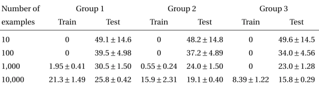
The performance of the AdaBoost classifier increases strictly with both the number of training examples and the complexity of the features. The test error decreases logarithmically with the number of training examples on all the problems, for example using all the features the mean test errors across all problems are 49.6%, 34.0%, 23.0%, and 15.8% training respectively with 10, 100, 1,000, and 10,000 examples, as can be read in the last column of table 2.1. Considering that a problem is ‘solved’ when its associated test error drops below 10%, no problem are solved training with only 10 examples, 2 when training with 100 examples, 10 when training with 1,000 examples, and 11 when training with 10,000 examples. The features used are also of importance, as the mean test error using the basic black pixel counting features of group 1 only drops from 25.8% to 19.1% when using also the edge related features of group 2, and to 15.8% when using also the spectral features of group 3. Although the performance does not strictly increase when using additional features (probably because of overfitting), it is very close to be the case. Using the same criteria as previously, it is this time 2 problems which can be solved using features from group 1, 8 when using group 2, and 11 using group 3.
The interpretation of these results is extremely difficult, as machine learning may rely on cues which seem at first irrelevant to the actual structure of the problem. For instance, images from problem 8 contain two closed shapes of different sizes. In positive images, the small shape is enclosed by the larger one, while in negative images they stand next to each others. While the rule involves reasoning about the spatial relations of the shapes, they can be approximately separated looking only at the distribution of the black pixels, which will be more concentrated for positive images and more spread out for negatives. Simply thresholding the variance of the pixels leads to a 9% test error, already ‘solving’ the problem. Symmetry with respect to a centered axis induces a more balanced repartition of the black pixels, as they can not anymore be all located on one side of the said axis, although Fourier features also seem to be able to help with the problem quite a bit.
All these cues provide information about the state of interest, but have a very indirect relation to the underlying rule. In the end, a few exact geometrical properties are probably perceived by the classification algorithm through a multitude of slightly unbalanced statistical cues.
2.2. Experiments 0 0.1 0.2 0.3 0.4 0.5 102 10 103 4102 10 103 4102 10 103 4 102 10 103 4102 10 103 4102 10 103 4 102 10 103 4102 10 103 4102 10 103 4 102 10 103 4102 10 103 4102 10 103 4 cumulated errors (a) Problem 1. 0 0.1 0.2 0.3 0.4 0.5 102 10 103 4102 10 103 4102 10 103 4 102 10 103 4102 10 103 4102 10 103 4 102 10 103 4102 10 103 4102 10 103 4 102 10 103 4102 10 103 4102 10 103 4 cumulated errors (b) Problem 2. 0 0.1 0.2 0.3 0.4 0.5 102 10 103 4102 10 103 4102 10 103 4 102 10 103 4102 10 103 4102 10 103 4 102 10 103 4102 10 103 4102 10 103 4 102 10 103 4102 10 103 4102 10 103 4 cumulated errors (c) Problem 3. 0 0.1 0.2 0.3 0.4 0.5 102 10 103 4102 10 103 4102 10 103 4 102 10 103 4102 10 103 4102 10 103 4 102 10 103 4102 10 103 4102 10 103 4 102 10 103 4102 10 103 4102 10 103 4 cumulated errors (d) Problem 4. 0 0.1 0.2 0.3 0.4 0.5 102 10 103 4102 10 103 4102 10 103 4 102 10 103 4102 10 103 4102 10 103 4 102 10 103 4102 10 103 4102 10 103 4 102 10 103 4102 10 103 4102 10 103 4 cumulated errors (e) Problem 5. 0 0.1 0.2 0.3 0.4 0.5 102 10 103 4102 10 103 4102 10 103 4 102 10 103 4102 10 103 4102 10 103 4 102 10 103 4102 10 103 4102 10 103 4 102 10 103 4102 10 103 4102 10 103 4 cumulated errors (f ) Problem 6. 0 0.1 0.2 0.3 0.4 0.5 102 10 103 4102 10 103 4102 10 103 4 102 10 103 4102 10 103 4102 10 103 4 102 10 103 4102 10 103 4102 10 103 4 102 10 103 4102 10 103 4102 10 103 4 cumulated errors (g) Problem 7. 0 0.1 0.2 0.3 0.4 0.5 102 10 103 4102 10 103 4102 10 103 4 102 10 103 4102 10 103 4102 10 103 4 102 10 103 4102 10 103 4102 10 103 4 102 10 103 4102 10 103 4102 10 103 4 cumulated errors (h) Problem 8. 0 0.1 0.2 0.3 0.4 0.5 102 10 103 4102 10 103 4102 10 103 4 102 10 103 4102 10 103 4102 10 103 4 102 10 103 4102 10 103 4102 10 103 4 102 10 103 4102 10 103 4102 10 103 4 cumulated errors (i) Problem 9. 0 0.1 0.2 0.3 0.4 0.5 102 10 103 4102 10 103 4102 10 103 4 102 10 103 4102 10 103 4102 10 103 4 102 10 103 4102 10 103 4102 10 103 4 102 10 103 4102 10 103 4102 10 103 4 cumulated errors (j) Problem 10. 0 0.1 0.2 0.3 0.4 0.5 102 10 103 4102 10 103 4102 10 103 4 102 10 103 4102 10 103 4102 10 103 4 102 10 103 4102 10 103 4102 10 103 4 102 10 103 4102 10 103 4102 10 103 4 cumulated errors (k) Problem 11. 0 0.1 0.2 0.3 0.4 0.5 102 10 103 4102 10 103 4102 10 103 4 102 10 103 4102 10 103 4102 10 103 4 102 10 103 4102 10 103 4102 10 103 4 102 10 103 4102 10 103 4102 10 103 4 cumulated errors (l) Problem 12. 0 0.1 0.2 0.3 0.4 0.5 102 10 103 4102 10 103 4102 10 103 4 102 10 103 4102 10 103 4102 10 103 4 102 10 103 4102 10 103 4102 10 103 4 102 10 103 4102 10 103 4102 10 103 4 cumulated errors (m) Problem 13. 0 0.1 0.2 0.3 0.4 0.5 102 10 103 4102 10 103 4102 10 103 4 102 10 103 4102 10 103 4102 10 103 4 102 10 103 4102 10 103 4102 10 103 4 102 10 103 4102 10 103 4102 10 103 4 cumulated errors (n) Problem 14. 0 0.1 0.2 0.3 0.4 0.5 102 10 103 4102 10 103 4102 10 103 4 102 10 103 4102 10 103 4102 10 103 4 102 10 103 4102 10 103 4102 10 103 4 102 10 103 4102 10 103 4102 10 103 4 cumulated errors (o) Problem 15. 0 0.1 0.2 0.3 0.4 0.5 102 10 103 4102 10 103 4102 10 103 4 102 10 103 4102 10 103 4102 10 103 4 102 10 103 4102 10 103 4102 10 103 4 102 10 103 4102 10 103 4102 10 103 4 cumulated errors (p) Problem 16.
0 0.1 0.2 0.3 0.4 0.5 102 10 103 4102 10 103 4102 10 103 4 102 10 103 4102 10 103 4102 10 103 4 102 10 103 4102 10 103 4102 10 103 4 102 10 103 4102 10 103 4102 10 103 4 cumulated errors (q) Problem 17. 0 0.1 0.2 0.3 0.4 0.5 102 10 103 4102 10 103 4102 10 103 4 102 10 103 4102 10 103 4102 10 103 4 102 10 103 4102 10 103 4102 10 103 4 102 10 103 4102 10 103 4102 10 103 4 cumulated errors (r) Problem 18. 0 0.1 0.2 0.3 0.4 0.5 102 10 103 4102 10 103 4102 10 103 4 102 10 103 4102 10 103 4102 10 103 4 102 10 103 4102 10 103 4102 10 103 4 102 10 103 4102 10 103 4102 10 103 4 cumulated errors (s) Problem 19. 0 0.1 0.2 0.3 0.4 0.5 102 10 103 4102 10 103 4102 10 103 4 102 10 103 4102 10 103 4102 10 103 4 102 10 103 4102 10 103 4102 10 103 4 102 10 103 4102 10 103 4102 10 103 4 cumulated errors (t) Problem 20. 0 0.1 0.2 0.3 0.4 0.5 102 10 103 4102 10 103 4102 10 103 4 102 10 103 4102 10 103 4102 10 103 4 102 10 103 4102 10 103 4102 10 103 4 102 10 103 4102 10 103 4102 10 103 4 cumulated errors (u) Problem 21. 0 0.1 0.2 0.3 0.4 0.5 102 10 103 4102 10 103 4102 10 103 4 102 10 103 4102 10 103 4102 10 103 4 102 10 103 4102 10 103 4102 10 103 4 102 10 103 4102 10 103 4102 10 103 4 cumulated errors (v) Problem 22. 0 0.1 0.2 0.3 0.4 0.5 102 10 103 4102 10 103 4102 10 103 4 102 10 103 4102 10 103 4102 10 103 4 102 10 103 4102 10 103 4102 10 103 4 102 10 103 4102 10 103 4102 10 103 4 cumulated errors (w) Problem 23.
Figure 2.2 – The training and testing errors (in resp. orange and yellow), as well as the standard deviations (in resp. dark blue and light blue) on each of the 23 image classification problems making up the Synthetic Visual Reasoning Test (SVRT). There are 3 groups of 3 histograms for each of the problem. Each group corresponds to the respective group of features, while the 3 histograms in a group corresponds to different amount of training examples (102, 103, 104). No histogram for 101examples as the errors are all 0 in training and 0.5 in testing.
Table 2.1 – Mean training and testing errors with their standard deviations (all in percent) on all 23 problems of the Synthetic Visual Reasoning Test (SVRT), for the 3 feature groups and different numbers of training examples.
Number of Group 1 Group 2 Group 3
examples Train Test Train Test Train Test
10 0 49.1±14.6 0 48.2±14.8 0 49.6±14.5
100 0 39.5±4.98 0 37.2±4.89 0 34.0±4.56
1,000 1.95±0.41 30.5±1.50 0.55±0.24 24.0±1.50 0 23.0±1.28
2.3. Conclusion
We also performed the same experiments using a Support Vector Machine (SVM) (Vapnik, 1995) with a Gaussian kernel, concatenating all the features together. We do not report the results as they show the same trends that the ones of figure 2.2, and are on average weaker (probably because the features were not weighted optimally).
The machine learning techniques we used for this study do not interpret the images as a configuration of parts, each with its own variability, and with a complex model of their relative positioning. That is why comparison with human subjects is embarrassing for the machine learning classifier, as most participants could solve all problems looking at a few pairs of examples only.
2.3 Conclusion
Both the number of training examples and the amount of features are critical to obtain good performances. Increasing the number of features is the most direct strategy to reduce the gap between humans and machine learning algorithms. The training time increasing at least linearly with both, it is crucial to develop smarter training algorithms, able to train a classifier efficiently in large scale scenarios.
3
Adaptive Sampling for Large Scale
Boosting
In this chapter we present our contributions to reduce the training time of Boosting algorithms. Classical algorithms, such as AdaBoost, build a strong classifier without concern for the com-putational cost. Some applications, in particular in computer vision, may involve millions of training examples and very large feature spaces. In such contexts, the training time of off-the-shelf Boosting algorithms may become prohibitive. Several methods exist to accelerate training, typically either by sampling the features or the examples used to train the weak learners. Even if some of these methods provide a guaranteed speed improvement, they offer no insurance of being more efficient than any other, given the same amount of time.
Our contributions are twofold: (a) a strategy to better deal with the increasingly common case where features come from multiple sources (e.g.color, shape, texture,etc., in the case of images) and therefore can be partitioned into meaningful subsets; (b) new algorithms which estimate at every Boosting iteration the optimal trade-off between the number of weak learners and the number of training examples to look at in order to maximize the expected loss reduction. Experiments in image classification and object recognition on four standard computer vision datasets show that the adaptive methods we propose outperform basic sampling and state-of-the-art bandit methods. Content presented in this chapter is based on the following publications (Dubout and Fleuret, 2011a,b):
C. Dubout and F. Fleuret. Tasting families of features for image classification. In Interna-tional Conference on Computer Vision, 2011.
C. Dubout and F. Fleuret. Boosting with maximum adaptive sampling. InNeural Infor-mation Processing Systems, 2011.
3.1. Introduction
3.1 Introduction
Boosting is a simple and efficient machine learning algorithm which provides state-of-the-art performance on many tasks. It consists of building a strong classifier as a linear combination of weak learners, by adding them one after another in a greedy manner.
It has been repeatedly demonstrated that combining multiple kind of features addressing different aspects of the signal is an extremely efficient strategy to improve performance (Opelt et al., 2006; Gehler and Nowozin, 2009; Dubout and Fleuret, 2011a,b). As shown by our experimental results, vanilla Boosting of stumps over multiple image features such as HOG, LBP, color histograms,etc., usually reaches close to state-of-the-art performance. However, such techniques entails a considerable computational cost, which increases with the number of features considered during training.
The critical operations contributing to the computational cost of a Boosting iteration are the computations of the features and the selection of the weak learner. Both depend on the number of features and the number of training examples taken into account. While textbook AdaBoost repeatedly selects each weak learner using all the features and all the training examples for a predetermined number of rounds, one is not obligated to do so and can instead choose to look only at a subset of both.
Since performance increases with both, one needs to balance the two to keep the computa-tional cost under control. As Boosting progresses, the performance of the candidate weak learners degrades, and they start to behave more and more similarly. While a small number of training examples is initially sufficient to characterize the good ones, as the learning problems become more and more difficult, optimal values for a fixed computational cost tend to move towards smaller number of features and larger number of examples.
In this paper, we present three new families of algorithms to explicitly address these issues: (1) Tasting (see § 3.4) uses a small number of features sampled prior to learning to adaptively bias the sampling towards promising subsets at every step; (2) Maximum Adaptive Sampling (see § 3.5.3) models the distribution of the weak learners’ performance and the noise in order to determine the optimal trade-off between the number of weak learners and the number of examples to look at; and (3) Laminating (see § 3.5.4) iteratively refines the learner selection using more and more examples.
3.2 Related works
AdaBoost and similar Boosting algorithms estimate for each candidate weak learner a score dubbed “edge”, which requires to loop through every training example and take into account its weight, which reflects its current importance in the loss reduction. Reducing this computa-tional cost is crucial to cope with high-dimensional feature spaces or very large training sets. This can be achieved through two main strategies: sampling the training examples, or the
feature space, since there is a direct relation between features and weak learners.
Sampling the training set was introduced historically to deal with weak learners which cannot be trained with weighted examples (Freund and Schapire, 1996). This procedure consists of sampling examples from the training set according to their Boosting weights, and of ap-proximating a weighted average over the full set by a non-weighted average over the sampled subset. It is related to Bootstrapping as similarly the training algorithm will sample harder and harder examples based on the performance of the previous weak learners. See § 3.3 for formal details. Such a procedure has been re-introduced recently for computational reasons (Bradley and Schapire, 2007; Duffield et al., 2007; Kalal et al., 2008; Fleuret and Geman, 2008), since the number of sampled examples controls the trade-off between statistical accuracy and computational cost.
Sampling the feature space is the central idea behind LazyBoost (Escudero et al., 2000), and simply consists of replacing the brute-force exhaustive search over the full feature set by an optimization over a subset produced by sampling uniformly a predefined number of features. The natural redundancy of most type of features makes such a procedure generally efficient. However, if a subset of important features is too small, it may be overlooked during training. Recently developed algorithms rely on multi-arms bandit methods to balance properly the exploitation of features known to be informative, and the exploration of new features (Busa-Fekete and Kegl, 2009, 2010). The idea behind those methods is to associate a bandit arm to every feature, and to see the loss reduction as a reward. Maximizing the overall reduction is achieved with a standard bandit strategy such as UCB (Auer et al., 2002), or Exp3.P (Auer et al., 2003).
These techniques suffer from two important drawbacks. First they make the assumption that the quality of a feature – the expected loss reduction of a weak learner using it – is stationary. This goes against the underpinning of Boosting, which is that at any iteration the performance of the weak learners is relative to the Boosting weights, which evolve over the training (Exp3.P does not make such an assumption explicitly, but still rely exclusively on the history of past rewards). Second, without additional knowledge about the feature space, the only structure they can exploit is the stationarity of individual features. Hence, improvement over random selection can only be achieved by sampling againthe exact same featuresalready seen in the past. In our experiments, we therefore only use those methods in a context where features can be partitioned into subsets of different types. This allows us to model the quality, and thus to bias the sampling, at a higher level than individual features.
All those approaches exploit information about features to bias the sampling, hence making it more efficient, and reducing the number of weak learners required to achieve the same loss reduction. However, they do not explicitly aim at controlling the computational cost. In particular, there is no notion of varying the number of examples used for the estimation of the loss reduction.
3.3. Preliminaries
3.3 Preliminaries
We first present in this section some analytical results to approximate a standard round of AdaBoost – or other similar Boosting algorithms – by sampling both the training examples and the features used to build the weak learners. We then precise more formally what we mean by subset of features or weak learners.
3.3.1 Standard Boosting Given a binary training set
(xn,yn)∈X×{−1, 1},n=1, . . . ,N (3.1)
whereX is the space of the “visible” signal, and a setH of weak learners of the formh:X→
{−1, 1}, the standard Boosting procedure consists of building a strong classifier
f = T X t=1
αtht (3.2)
by choosing the termsαt ∈Randht ∈H in a greedy manner so as to minimize a loss (e.g.
the empirical exponential loss in the case of AdaBoost) estimated over the training examples. At every iteration, choosing the optimal weak learner boils down to finding the one with the largest edge², which is the derivative of the loss reduction w.r.t. the weak learner weightα. The higher this value, the more the loss can be reduced locally, and thus the better the weak learner. The edge is a linear function of the responses of the weak learner over the training examples ²(h)= N X n=1 ω(n)ynh(xn) (3.3)
where the weightsω(n)s depend on the loss function (usually either the exponential or logistic loss) and on the current responses off over thexns. We consider without loss of generality that
they have been normalized such thatPN
n=1ω(n)=1. We can therefore consider the weights
ω(n)s as a distribution over the training examples and rewrite the edge as an expectation
²(h)=EN∼ω(n)£yNh(xN)¤ (3.4)
whereN∼ω(n) stands for P(N=n)=ω(n). The idea of weighting-by-sampling (Fleuret and Geman, 2008) consists of replacing the expectation in (3.4) with an approximation obtained by sampling. LetN1, . . . ,NS, be i.i.d. random variables distributed according to the discrete
probability density distribution defined by theω(n)s, we define the approximated edge as ˆ ²(h)=1 S S X s=1 yNsh(xNs) (3.5)
which follows a binomial distribution centered on the true edge, with a variance decreasing with the number of sampled examplesS. It is accurately modeled by the Gaussian
ˆ ²(h)≈N µ ²(h),(1+²(h))(1−²(h)) S ¶ (3.6) as the approximation holds asymptotically and the magnitude of the weak learners’ edges is typically small, such that (1+²(h))(1−²(h))≈1.
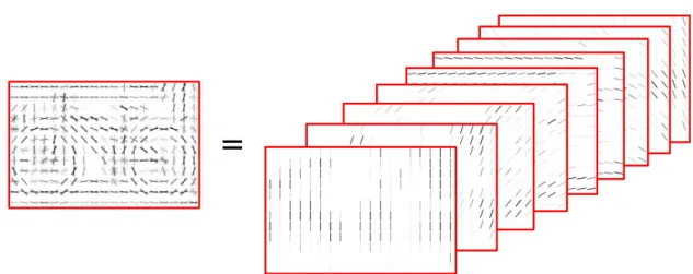
3.3.2 Feature subsets
It frequently happens that the features making up the signal spaceX can be divided into meaningful disjoint subsetsFksuch thatX = ∪Kk=1Fk. This division can for example be the
result of the features coming from different sources or some natural clustering of the feature space. In such a case it makes sense to use this information during training, as features coming from the same subsetFkcan typically be expected to be more homogeneous than features
coming from different subsets.
3.4 Tasting
We describe here our approach called Tasting (Dubout and Fleuret, 2011a) which biases the sampling toward promising subsets of features. Tasting in its current form is limited to deal with weak learner looking at only one feature, such as decision stumps. Extending it to deal efficiently with weak learners looking at multiple features is outside of the scope of this work.
3.4.1 Main algorithm
The core idea of Tasting is to sample a small numberRof features from every subset before starting the trainingper seand, at every Boosting step, in using these few features together with the current Boosting weights to get an estimate of the best subset(s)Fk(s) to use.
We cannot stress enough that theseRfeatures are not the ones used to build the classifier, they are only used to figure out what is/are the best subset(s) at any time during training. As those sampled features are independent and identically distributed samples of the feature response vectors, we can compute the empirical mean of any functional of the said response vectors, in particular the expected loss reduction.
At any Boosting step, Tasting require, for any feature subset, an estimate of the expectation of the edge of the best weak learner we would obtain by sampling uniformlyQfeatures from this subset and picking the best weak learner using one of them,
EF1,...,FQ∼U(Fk) " Q max q=1hmax∈HFq ²(h) # (3.7)
3.4. Tasting
Algorithm 3.1The Tasting 1.Q algorithm first samples uniformlyRfeatures from every subset Fk. It uses these features at every Boosting step to find the optimal feature subsetk∗from
which to sample. After the selection of theQfeatures, the algorithm continues like AdaBoost.
Input: F,Q,R,T Initialize: ∀k∈{1, . . . ,K},∀r∈{1, . . . ,R},frk←sample(U(Fk)) fort=1, . . . ,T do ∀k∈{1, . . . ,K},∀r∈{1, . . . ,R},²kr← max h∈Hf kr ²(h) k∗←argmax k E · Q max q=1 ² k Rq ¸
# Computed using equation (3.10)
∀q∈{1, . . . ,Q},Fq←sample(U(Fk∗)) ht←argmax h∈∪qHFq ²(h) . . . end for
whereFk are the indices of the features belonging to thek-th subset andHF is the space
of weak learners looking solely at featureF. Hence maxh∈HFq²(h) is the best weak learner
looking solely at featureFq, and maxQq=1maxh∈HFq²(h) is the best weak learner looking solely
at one of theQfeaturesF1, . . . ,FQ.
We can build an approximation of this quantity using theR features we have stored. Let ²1, . . . ,²R be the edges of the bestRweak learners built from these features. We make the
assumption without loss of generality that²1≤²2≤ · · · ≤²R. LetR1, . . . ,RQbe independent
and identically distributed, uniform over {1, . . . ,R}. We approximate the quantity (3.7) with
E · Q max q=1 ²Rq ¸ = R X r=1 P µ Q max q=1 Rq=r ¶ ²r (3.8) = R X r=1 · P µ Q max q=1 Rq≤r ¶ −P µ Q max q=1 Rq≤r−1 ¶¸ ²r (3.9) = 1 RQ R X r=1 £ rQ−(r−1)Q¤ ²r. (3.10) 3.4.2 Tasting variants
We propose two versions of the Tasting procedure, which differ in the number of feature subsets they visit at every iteration. Either one for Tasting 1.Q or up toQfor Tasting Q.1.
In Tasting 1.Q (algorithm 3.1), the selection of the optimal subsetk∗from which to sample the
Qfeatures is accomplished by estimating for every subset the expected maximum edge, which is directly related to the expected loss reduction, if we were sampling from that subset only. The computation is done over theRfeatures saved before starting training, which serve as a representation of the full setFk.
Algorithm 3.2The Tasting Q.1 algorithm similarly starts by sampling uniformlyRfeatures from every subsetFk, but it then uses them to find the optimal subsetk∗q for every one of the
Qfeatures to sample at every Boosting step. After the selection of theQfeatures, the algorithm continues like AdaBoost.
Input: F,Q,R,T Initialize: ∀k∈{1, . . . ,K},∀r∈{1, . . . ,R},frk←sample(U(Fk)) fort=1, . . . ,T do ∀k∈{1, . . . ,K},∀r∈{1, . . . ,R},²kr← max h∈Hf k r ²(h) ²∗←0 forq=1, . . . ,Qdo kq∗←argmax k Ehmax³²∗,²k´i Fq←sample ³ U³Fk∗ q ´´ ²∗←max à ²∗, max h∈HFq ²(h) ! end for ht←argmax h∈∪qHFq ²(h) . . . end for
In Tasting Q.1 (see algorithm 3.2), it is not one but several feature subsets which can be selected, as the algorithm picks the best subsetk∗qfor every one of theQfeatures to sample,
given the best edge²∗achieved so far. Again the computation is done only over theRfeatures saved before starting training.
3.4.3 Relation with Bandit methods
The main strength of Boosting is its ability to spot and combine complementary features. If the loss has already been reduced in a certain “functional direction”, the scores of weak learners in the same direction will be low, and they will be rejected. For instance, the firsts learners for a face detector may use color-based features to exploit the skin color. After a few Boosting steps using this modality, color would be would be exhausted as a source of information, and only examples with a non-standard face color would have large weights. Other features, for instance edge-based, would become more informative, and be picked.
Uniform sampling of features accounts poorly for such behavior since it simply discards the Boosting weights, and hence has no information whatsoever about the directions which have “already been exploited” and which should be avoided. In practice, this means that the rejection of bad feature can only be done at the level of the Boosting itself, which may end up with a majority of useless features.
3.5. Maximum Adaptive Sampling and Laminating
Bandit methods (described in § 3.6.4) are slightly more adequate, as they model the perfor-mance of every feature from previous iterations. However, this modeling takes into account the Boosting weights very indirectly, as they make the assumption that the distributions of loss reduction are stationary, while they are precisely not. Coming back to our face-detector example, bandit methods would go on believing that color is informative since it was in the previous iterations, even if the Boosting weights have specifically accumulated on faces where color is now totally useless. While the estimate of loss reduction may asymptotically converge to an adequate model, it is a severe weakness while the Boosting weights are still evolving. Tasting addresses this weakness by keeping the ability to properly estimate the performance of every feature subset,given the current Boosting weights, hence the ability to discard feature subsets redundant with features already picked. In some sense, Tasting can be seen as Boosting done at a the subset level.
3.5 Maximum Adaptive Sampling and Laminating
The algorithms in this section sample both the weak learners and the training examples at every iteration in order to maximize the expectation of the loss reduction, under a strict computational cost constraint.
3.5.1 Edge estimation
At every iteration they model the expectation of the edge of the selected weak learner. Let ²1, . . . ,²Qstand for the true edges ofQindependently sampled weak learners. Let∆1, . . . ,∆Q
be a series of independent random variables standing for the noise in the estimation of the edges due to the sampling of onlyStraining examples. Finally∀q, let ˆ²q =²q+∆q be the
approximated edge. With these definitions, argmaxq²ˆqis the selected weak learner. We define
²∗as the true edge of the selected weak learner, that is the one with the highest approximated edge
²∗=²
argmaxq²ˆq. (3.11)
This quantity is random due to both the sampling of the weak learners, and the sampling of the training examples. The quantity we want to optimize is E[²∗], the expectation of the true edge of the selected learner, which increases with bothQ andS. A higherQincreases the number of terms in the maximization of (3.11), while a higherSreduces the variance of the ∆s, ensuring that²∗is closer to maxq²q. In practice, if the variance of the∆s is of the order of, or higher than, the variance of the²s, the maximization is close to a random selection, and
1 10 100 1,000 10,000 1 10 100 1,000 10,000 0 0.1 0.2 0.3 0.4 Number of examples S Number of features Q Expectation 1 10 100 1,000 10,000 1 10 100 1,000 10,000 0 0.1 0.2 0.3 0.4 Number of examples S Number of features Q Expectation 1 10 100 1,000 10,000 0 1 2 3 4 Number of features Q
Expectation for a given cost QS
QS = 1,000 QS = 10,000 QS = 100,000 1 10 100 1,000 10,000 0 1 2 3 4 Number of features Q
Expectation for a given cost QS
QS = 1,000 QS = 10,000 QS = 100,000 Expectation QS = 1,000 QS = 10,000 QS = 100,000 Expectation QS = 1,000 QS = 10,000 QS = 100,000
Figure 3.1 – Simulation of the expectation of²∗in the case where both the²qs and the∆qs
follow Gaussian distributions. Top: ²q ∼N(0, 10−2). Bottom: ²q ∼N(0, 10−4). In both
simulations∆q∼N(0,S1). Left: expectation of²∗vs. the number of sampled learnersQand
the number of examplesS. Right: same value as a function ofQalone, for different fixed costs (product ofQandS). As these graphs illustrate, the optimal value forQis greater for larger variances of the²qs. In such a case the²qs are more spread out, and identifying the largest one
can be done despite a large noise in the estimations, hence with a limited number of training examples.
looking at many weak learners is useless. Assuming that the ˆ²qs are all different we have
E[²∗]=Eh²argmaxq²ˆq i (3.12) = Q X q=1 E " ²q Y i6=q 1{ˆ²i<ˆ²q} # (3.13) = Q X q=1 E " E " ²q Y i6=q 1{ˆ²i<²ˆq} ¯ ¯ ¯ ¯ ¯ ˆ ²q ## (3.14) = Q X q=1 E " E£ ²q¯¯²ˆq¤ Y i6=q E£ 1{ˆ²i<²ˆq} ¯ ¯²ˆq¤ # (3.15)
where the last equality follows from the independence of the weak learners.