Gene Regulatory Network Inference Using Machine Learning Techniques

(1)

GENE REGULATORY NETWORK INFERENCE USING

MACHINE LEARNING TECHNIQUES

Stephanie Kamgnia Wonkap

A Thesis in

the department of

Computer Science and Software Engineering

Presented in Partial Fulfillment of the Requirements For the Degree of Doctor of Philosophy(Computer Science)

Concordia University Montr´eal, Qu´ebec, Canada

August 26 2020 c

(2)

Concordia University

School of Graduate Studies

This is to certify that the thesis prepared

By: Miss. Stephanie Kamgnia Wonkap

Entitled: Gene Regulatory Network Inference using Machine Learning Techniques

and submitted in partial fulfillment of the requirements for the degree of

Doctor of Philosophy (Computer Science)

complies with the regulations of this University and meets the accepted standards with respect to originality and quality.

Signed by the final examining committee:

Chair Dr. Liangzhu Wang External Examiner Dr. Mathieu Blanchette Examiner Dr. Leila Kosseim Examiner Dr. Malcolm Whiteway Examiner Dr. Volker Haarslev Supervisor Dr. Gregory Butler Approved Dr. Leila Kosseim,

Graduate Program Director

August 26th, 2020

(3)

Abstract

Gene Regulatory Network Inference using Machine Learning

Techniques

Stephanie Kamgnia Wonkap, Ph.D. Concordia University, 2020

Systems Biology is a field that models complex biological systems in order to better understand the working of cells and organisms. One of the systems modeled is the gene regulatory network that plays the critical role of controlling an organism’s response to changes in its environment. Ideally, we would like a model of the complete gene regulatory network. In recent years, several advances in technology have permitted the collection of an unprecedented amount and variety of data such as genomes, gene expression data, time-series data, and perturbation data. This has stimulated research into computational methods that reconstruct, or infer, models of the gene regulatory network from the data. Many solutions have been proposed, yet there remain open challenges in utilising the range of available data as it is inherently noisy, and must be integrated by the inference techniques. The thesis seeks to contribute to this discourse by investigating challenges of performance, scale, and data integration.

We propose a new algorithm BENIN that views network inference as feature se-lection to address issues of scale, that uses elastic net regression for improved per-formance, and adapts elastic net to integrate different types of biological data. The

BENINalgorithm is benchmarked on a synthetic dataset from the DREAM4 challenge, and on real expression data for the human HeLa cell cycle. On the DREAM4 dataset

BENIN out-performed all DREAM4 competitors on the size 100 subchallenge, and is also competitive with more recent state-of-the-art methods. Moreover, on the HeLa cell cycle data, BENIN could infer known regulatory interactions and propose new interactions that warrant further experimental investigation.

Keys words: gene regulatory network, network inference, feature selection, elastic net regression.

(4)

Acknowledgments

First of all, I would like to thank my academic supervisor, Dr. Gregory Butler, for his precious advice that helped me accomplish this project and become a better researcher. Moreover, I would like to thank him for providing me with financial support.

I would like to thank my mother, Bernadette, and my father, Emmanuel, for showing the path through my Ph.D. Your prayer, love, and support helped go through these tough times. Thank you for your education that made me the strong woman I am today.

I would like to thank my sister Nathalie who is my model since our childhood. I made it I am a doctor like you. Thank you to my sister Helene who was always there, our phone calls, and our discussion helped during all these years. I will not forget my sister Diana, my nephews, my older brother Armand and two little brothers Joan and Gracien. Every one of you plays an essential role in this journey.

To you my beloved husband Samir, you were my rock through this journey. Thank you for holding my back, for being such a good confident and my motivation. I think that if you were not there, I would not be able to accomplish this. I thank God for having you in my life.

Last but not the less, my colleagues from office 11.411. I will never forget all these good times: the sushi time, our potluck dinner, our late discussions and all our fun time. I will miss these times and I wish you all the best in your life.

(5)

List of Figures

1 Organization of an operon in prokaryotes. . . 3

2 Tryptophan regulation in E. coli . . . 4

3 Eukaryotic gene structure . . . 6

4 Chromatin in eukaryotic cells . . . 7

5 Gene regulatory network abstraction . . . 8

6 Different representations of binding sites . . . 29

7 DNA microarray experiment . . . 35

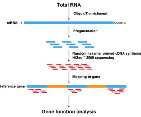
8 RNA-seq experiment . . . 37

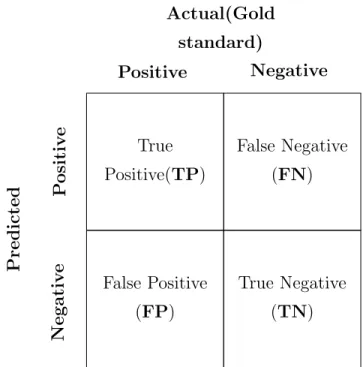
9 Confusion matrix . . . 41

10 Procedure to identify regulon . . . 51

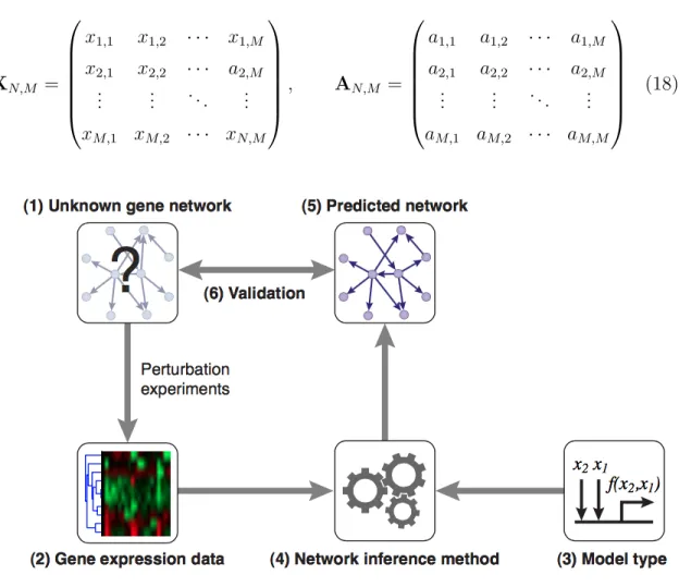
11 Step for regulatory network inference. . . 58

12 Example DREAM4 Input for BENIN . . . 84

13 Effect of the noise in location data . . . 99

14 Influence of BENIN parameters . . . 100

15 A subnetwork from 100-nodes network 4 . . . 109

16 The Eukaryotic cell cycle . . . 125

17 From nucleus to DNA sequence . . . 126

18 Steps for retrieving knockdown data . . . 140

19 Steps for collecting promoter sequences . . . 142

20 Steps for collecting protein sequences . . . 144

22 Snapshot of FIMO output . . . 153

24 Inference of GRN controlling HeLa cell cycle throughBENIN . . . 157

21 BED file and BETA-minus output . . . 160

23 Differential Expression analysis output . . . 161

(8)

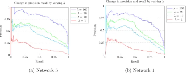
26 Precision-recall curves for BENIN . . . 163

27 ROC curves for BENIN . . . 165

28 Precision-recall curves for BENIN +orthology . . . 167

29 ROC curves for BENIN +orthology . . . 167

30 Orthologous Regulatory Network From mouse . . . 180

31 Edge Distribution . . . 181

32 Global score Distribution for the DREAM4 size 100 subchallenge. . . 233

(9)

List of Tables

1 Motifs Finding Methods . . . 52

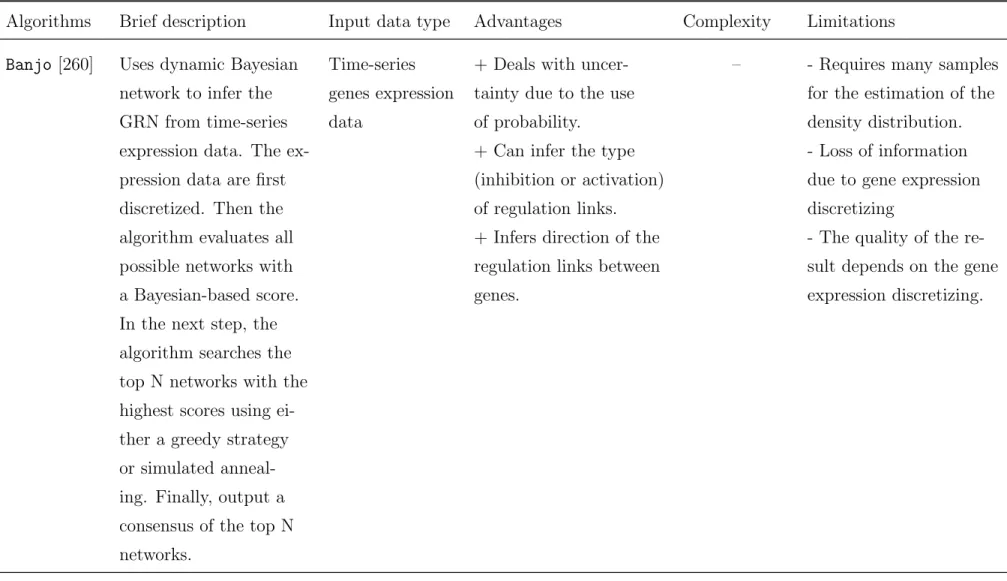
2 Reverse-Engineering Methods . . . 71

3 Description of DREAM4 size 10 and size 100 networks . . . 91

4 Motifs and errors type . . . 94

5 BENIN execution time on the DREAM4 . . . 96

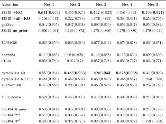
6 DREAM4 size 100 performance with KO expression . . . 103

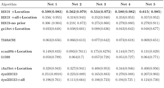
7 DREAM4 size 100 performance with Location data . . . 104

8 Global score on the DREAM4 size 100 subchallenge . . . 105

9 DREAM4 size 10 performance with Location data . . . 106

10 DREAM4 size 10 performance with KO expression . . . 106

11 Global score on the DREAM4 size 10 subchallenge . . . 107

12 Motif prediction confidence (median rank) . . . 113

13 Cell cycle Transcription Factors . . . 127

14 Characteristics of our Human “gold-standard” network . . . 136

15 Missing transcription factors in our “gold-standard network” . . . 137

16 Mouse gene regulatory network . . . 146

17 BENIN execution time . . . 159

18 BENIN performance . . . 162

19 Transcription factor and target gene . . . 168

20 Inference fromBENIN +combined+max . . . 174

21 Inference fromBENIN +orthology . . . 182

22 List of Degenerate IUPAC base symbols . . . 227

23 BENIN General Parameter setting . . . 230

24 BENIN +KO parameters on size 100 subchallenge . . . 230

(10)

26 BENIN +KO parameters on size 10 subchallenge . . . 231

27 BENIN +Location data parameters on size 10 subchallenge . . . 232

28 List of HeLa Peak Files . . . 238

29 List of knockdown datasets . . . 239

30 Information Motif and Transcription Factor . . . 240

31 Cell cycle genes . . . 249

32 Cell Cycle Transcription factor . . . 251

33 Knockdown Data from Gene Expression Omnibus . . . 268

34 Edges repetition in networks from HumanBase . . . 270

35 Edges repetition in Garcia networks . . . 286

36 HeLa “gold-standard” network - Positive links . . . 302

37 HeLa “gold-standard” network- Negative links . . . 319

38 Duplicate regulatory interaction from TRRUST and RegNetwork . . . . 340

39 Edges duplicated in our mouse regulatory network . . . 340

(11)

List of Terms and Abbreviations

ACC Accurary.

AUPR Area Under the Precision Recall curve.

AUROC Area under Receiver Operating Characteristic.

Biological pathway series of actions among molecules in a cell that leads to a cer-tain product or a change in a cell

BLAST Basic Local Alignment Search Tool. It is a sequence database searching program which compares a nucleotide or protein query sequence against all sequences in a database.

ChIP Chromatin ImmunoPrecipitation

DNA DeoxyriboNucleic Acid. It is a long double stranded molecule made of nu-cleotides A, C, G and T that contains the genetic information necessary for the development, functioning and the reproduction of all known living thing.

DREAM Dialogue for Reverse Engineering Assessments and Methods.

EM Expectation Maximisation.

ENet Elastic Net.

Enzyme Macro molecule that accelerates, or catalyzes, chemical reactions.

E-value Expected value, is the number of different alignments with scores equivalent to or better than threshold that are expected to occur by chance in a database search. The lower the E-value, the more significant the score.

(12)

FASTA Text-based format for representing either nucleotide sequences or amino acid, in which base pairs or amino acids are represented using single-letter codes.

FDR False Discovery Rate.

FFL Feed Forward Loop.

FN False Negative.

FP False Positive.

Gap Refer to substitution or indel in a sequence, where indel can be insertion or deletion in the sequence.

Gene expression profile Describes the expression levels of a gene across a set of samples obtained for a particular array experiment design.

GENIE3 GEne Network Inference with Ensemble of trees.

GO Gene Ontology. It is a major bioinformatics initiative to unify the representation of gene and gene product attributes across all species.

GRN Gene Regulatory Network.

IUPAC International Union of Pure and Applied Chemistry. It is the universally-recognized authority on chemical nomenclature and terminology.

LASSO Least Absolute Shrinkage and Selection Operator.

MEME Multiple EM for Motif Elicitation.

NPV Negative Predictive Value.

Non-coding DNA Components of DNA that do not encode protein sequences or RNA.

ODE Ordinary Differential Equation.

(13)

Ontology Formal naming and definition of the types, properties, and interrelation-ships of the entities that really or fundamentally exist for a particular domain of interest.

Operon Set of genes situated next to each other and under the control of the same promoter and operator.

Organelle Specialized subunit within the cell that has a specific function.

Ortholog Orthologous sequences are sequences occurring in different species that diverge from a common ancestral sequence after speciation, the evolutionary process in which new species arise.

Paralogy Sequences are paralogous if they were created by a duplication event within the genome.

Phenotype Observable characteristics of the organism such as eye’s color/shape, the hair’s color and so on.

Phylogenetic tree Diagram that depicts the lines of evolutionary descent of differ-ent species, organisms, or genes from a common ancestor.

PK Prior Knowledge.

PPI Proteins Proteins Interaction.

PPV Positive Predictive Value.

PWM Position Weight Matrix.

Regulatory sequence Segment of non-coding DNA that is capable to control the increase or decrease of the expression of specific genes within an organism.

Regulon Set of genes or operons regulated by the same transcription factor.

RNA Ribonucleic acid, is a single stranded molecule made of nucleotides A, C, G and U. It plays a major role in protein synthesis as it is involved in the transcription, decoding, and translation of the genetic code to produce proteins.

(14)

System Biology Computational and mathematical modeling of complex biological network.

TG Target Gene. It is a gene that is regulated by a transcription factor is called targeted gene of this transcription factor.

TF Transcription Factor.

TFBS Transcription Factor Binding Site.

TIGRESS Trustful Inference of Gene REgulation using Stability Selection.

TN True Negative.

TP True Positive.

TPR True Positive Rate.

TFBS Transciption Factor Binding Site.

VAR Vector AutoRegressive.

Enhancer TO DO

Silencer TO DO

Histone TO DO

Chromatin TO DO

ANOVA Analysis Of Variance

MRMR Minimum Redundancy Maximum Relevance

LASSO Least Absolute Shrinkage and Selection Operator

DEG Differentially Expressed Gene

ChiP-seq Chromatin immunoprecipitation followed by sequencing

(15)

DBD DNA Binding Domain

CDK Cyclin Dependent Kinase

Sister Chromatid copies of a chromosome held at the centromere

Spindle fibers aggregate of microtubules that are formed during the cell cycle and that move the chromosomes.

Microtubule protein filament that ressembles hollow tube.

KO Knockout

KD Knock down

KNN K nearest neighbor

Peak calling computational method used to identify areas in a genome that have been enriched with aligned reads after performing ChIP-sequencing experiment

AWG ENCODE Analysis Working Group

IC Information Content

MICA Most Informative Common Ancestor

TSS Transcription Start Site

FDR False Discovery Rate

EM Expectation Maximization

k-mer sequence of length k

MCMC Markov Chain Monte Carlo

BMA Bayesian Model Averaging

GGM Graphical Gaussian Model

FPR False Positive Rate

DPI data processing inequality

(16)

Chapter 1

Introduction

All living organisms on the earth interact with other organisms and are regularly exposed to environmental factors in their habitats. These factors are varied, encom-passing temperature, oxygen level, nutrient and water availability, and in some cases, the presence of toxic elements. In response to variations in these factors, organisms need to develop features to survive. These features take the form of gene expression and regulation. The following thesis engages with the complexities of this process. The thesis will be grounded on three key questions: “What is gene expression?” “What does it means to regulate the expression of a gene?” and finally, “How do these processes work?”

System Biology, a discipline that is deeply rooted in biology, physics, chemistry, as well as in computer science and mathematics, provides a mechanism for modeling the complex networks of biologically relevant entities (DNA, RNA, proteins, or cells) and in so doing, provides an avenue for answering questions such as “How does a biological component interact with other components and its environment?”, “What regulates its function and in what manner?”, “What kind of properties emerge from these interactions?” and so one [240]. Thegene regulatory network (GRN)is an example of these complex networks. The GRN offers a path to understand parameters that contribute to a properly functioning cell. Moreover, GRN helps understanding interactions between different organisms as well as the interaction with their habi-tats. Thus, there is a strong need to model such a complex network for scientists to have abstract reasoning about its dynamics. Even though we now witness high-throughput experiments that produce a plethora of data, the question of modeling

(17)

and reconstructing a GRN remains largely unsolved and a big challenge in Systems Biology. The following thesis will contribute to the discourse on the problems of GRN reconstruction.

1.1

Gene Regulation

1.1.1

Prokaryotic Gene Regulation

A gene is a portion of DNA responsible for the physical and inheritable characteristics or the phenotype (e.g., the shape, the color, or the size) of all living organisms. It is the way biological information is transmitted through generations and the basis of heredity. Each organism has a certain number of genes, e.g E. coli, a bacteria, has between 4,000 and 5,500 known genes. Inside the cells of every living thing, after receiving a signal triggered by distinct factors, each gene is transcribed into mRNA, a kind of RNA, by an enzyme called RNA-polymerase through a process known as transcription. Through another process known as translation, the mRNA is then transformed into a polypeptide chain, a component of proteins responsible for the observable characteristics of the organism. Gene expression is the process (transcrip-tion + transla(transcrip-tion) in which the biological informa(transcrip-tion contained in a gene is used to synthesize the gene products, which are principally proteins.

To better present and understand the gene regulation process, we will consider the prokaryotes’ case, as it is the easiest to comprehend. A eukaryote is an organism whose cells contain a nucleus and other organelles enclosed within membranes,e.g hu-man. A prokaryote is a single-celled organism that lacks membrane-bound organelles such as bacteria. Usually, an organism does not produce all proteins simultaneously because different proteins are involved in different cellular processes. It is important to control how much a gene is expressed at any given time and when a gene is needed. Any disruption to this control can yield serious consequences. For example, it is im-portant for E. coli to control the levels of tryptophan (Trp), an essential amino acid for its survival. Hence, if its environment is lacking tryptophan, E. coli needs to syn-thesize the proteins necessary to produce the tryptophan. One can thus define gene regulationas the set of mechanisms used by the cell to control (increase or decrease)

(18)

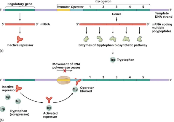
the products of gene expression. Figure 2 shows an example the Trp regulation in E. coli. In this figure, there are two types of genes. There are transcription factors (TFs) or regulatory genes, which are genes whose products control other genes’ expression. When those proteins increase the gene expression, they are calledactivators. Alter-natively, when proteins inhibit the expression of genes, we call them repressors. In Figure 2, there are also target genes (TGs) that are structural genes that encode pro-teins not involved in regulation. Gene regulation will manifest differently depending on whether the organism is a prokaryote or a eukaryote, as discussed in Section 1.1.2. In prokaryotes we identify specific regions of genes: operons,promoter regions and transcription factor binding sites (TFBS). Genes that produce proteins involved in the same process and are controlled by the same regulatory genes are located next to each other in clusters called operons. RNA polymerase will bind to a promoter region, a sub-region of the non-coding region upstream in an operon. A transcription factor binding site (TFBS), also known as an operator, is another non-coding sub-region where TFs will bind to allow gene regulation. Figure 1 summarizes the structure of a typical operon within prokaryotes.

Figure 1: Organization of an operon in prokaryotes.

Organization of genes in prokaryotes: related structural genes are situated next to each other, forming a cluster called an operon. The operon is under the control of a single promoter–where the RNA polymerase binds–and a single operator–where the TF will bind to control the expression of genes within the operon. This TF comes from the expression of the regulatory gene. The set formed by the promoter, the operator, and the structural genes is called operon [189].

(19)

Figure 2: Tryptophan regulation in E. coli

The tryptophan regulation in E. coli. In (a), the tryptophan is absent in the environment of E. coli. A repressor is made from a regulatory gene. However, as the environment lacks trp, it is inactive; thus, it does not bind to the operator. The RNA polymerase can thus transcribe the genes (structural genes) in the operon, and enzymes (here proteins) for the synthesis of tryptophan will be produced. (b)The environment of E. coli contains tryptophan, the repressor is active and can thus bind to the operator and block the activity of the RNA polymerase [189].

(20)

1.1.2

Eukaryotic Gene Regulation

As in prokaryotes, the process of gene regulation is controlled by proteins which at specific region allow or block the activity of RNA polymerase. However, in eukaryotic cells, gene regulation is far more complicated than in prokaryotic cells. First of all, eukaryotes have more genes than prokaryotes. Nearly all the cells of eukaryotes have the same DNA sequence. However, cell specialization is a result of the difference in gene regulation in these cells.

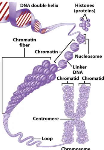
Another divergence is the organization of genes within the genome. Unlike prokary-otic cells, operons are generally not found in eukaryotes. Instead, each gene is as-sociated with its promoter element where the RNA polymerase and the regulatory protein will bind. The promoter is almost always situated upstream to the coding genes. Most of the time, transcription factor binding sites (TFBS) are located within promoter regions. However, in some cases, TFBS are located far from the promoter, either upstream or downstream from the coding region; they are called enhancers. It worth mentioning that in prokaryotic cells, the expression of genes may be controlled by the action of several TFs [144, 142]. In eukaryotes, gene expression is regulated at different levels, during transcription, and both before and after translation. It con-trasts with prokaryotes, where gene regulation happens primarily at the transcription level. Furthermore, a significant difference between the gene regulation in eukaryotic and prokaryotic cells is that, in eukaryotic cells, the DNA sequence is compacted around a protein called a histone, forming the nucleosome. Nucleosomes are assem-bled into a compact structure called chromatin. The chromatin can either promote or prevent genes regulation. TFs and RNA polymerase cannot access the target gene when the DNA is compacted around the histone. Figure 4 summarizes how the DNA is packed in the eukaryote genome.

1.2

Gene Regulatory Network

A gene regulatory network is a set of all elements (transcription factors, genes, or RNA) that interact together directly or indirectly to control genes’ expression. In this thesis, we will only consider the transcriptional level of regulation. Accordingly,

(21)

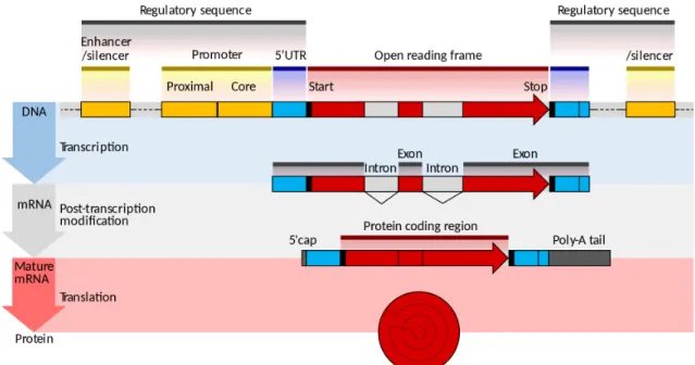
Figure 3: Eukaryotic gene structure

Organization of a gene within the genome of a eukaryote. The open reading frame contains the DNA sequence (target gene) transcribed by RNA polymerase. The promoter contains regions where a variety of TFs may bind, allowing the RNA polymerase to transcribe the adjacent gene: this is gene expression. Note that the RNA polymerase also binds in the promoter region, particularly in the core promoter region. Furthermore, the TFs can also bind in distant regions called enhancer or silencer regions, which also control gene expression.

(22)

Figure 4: Chromatin in eukaryotic cells

(23)

the gene regulatory network (GRN) will be the set of target genes (TGs) and tran-scription factors (TFs) that interact together through relations called regulatory links. Figure 5 shows a simplifying picture of the gene regulatory network consisting of a set of target genes and transcription factors and their regulatory interactions.

Figure 5: Gene regulatory network abstraction

The figure presents an abstraction of the gene regulatory network [193]. It consists of a set of genes, their expression products, and the regulatory interactions that exist between them.

Several studies [3, 4, 5] have demonstrated that, like many real networks, the out-degree of genes in the GRN follows a free distribution. Following a scale-free distribution indicates that most of the TFs are connected to a small number of genes, while only a few TFs regulate many genes. TFs that regulate a multitude of genes are called hub genes. This particular organization of the GRN ensures its connectivity and integrity [4, 5]. The presence of hub TFs in the GRN make it robust against random disruption [3], as they will generally affect non-hub genes, and, will consequently not lead to a loss of connectivity. Hubs are essential for the GRN and are generally the target of diseases like cancer. Given their importance, researchers have hypothesized that hub genes are subject to strict evolutionary constrains.

Apart from the gene connectivity distribution, the GRN has long been thought to have a modular organization that is a critical feature for the cell to coordinate its complex functions (the different tasks are split over the modules which can either interconnected or be insulated from) [95, 185]. Albert L`aszl`o et al have defined a module as a set of physically or functionally linked molecules that work together

(24)

to achieve distinct functions [11]. Given the GRN, a module will refer to a set of genes involved in a joint elementary function, sharing the same behavior (expression pattern) and under the control of a set of regulators that controls their expression. A gene can be part of multiple modules at a time, which implies that the functional modules overlap each other.

1.3

Problem Statement

Networks are omnipresent in biology and widely used to represent different kinds of information and most likely interactions. There exist several types of networks. For example, Protein-Protein networks that model the physical interactions of proteins or metabolic networks that comprehensively describe all possible biochemical reactions for an organism.

Gene expression regulation differs between eukaryotes and prokaryotes. In prokary-ote, the regulation is much simpler and happens at the transcription. However, in eukaryotes, gene expression regulation is more complex and happen at several levels:

• At the epigenetic level: i.e., when the DNA is unwound and loosened from the nucleosome to allow the transcriptional machinery to start the transcription

• At the transcriptional level, i.e., when the DNA is transcribed into RNA • At the post-transcriptional level, i.e., after the transcription but before the RNA

is translated into protein

• At the post-translational level, i.e., after the RNA is translated into proteins. In this work, we restrict the GRN at the transcriptional level where most of the genes are regulated [20]: it is the transcriptional gene regulatory network (TRN). The TRN offers a condensed view of the regulation. In what follows, the TRN represents the GRN. Restricting the expression to the transcriptional level. Restricting our model to transcription will ignore other types of regulation.

The GRN is generally represented as a graph. In this graph, the nodes are all the genes acting in the regulation or even modules of co-expressed genes. The graph can be directed or not. In this graph, a directed edge communicates the direct causal

(25)

relationship from a transcription factor (the source) to its target gene (the sink). Note that the edges can be signed, with a positive sign denoting activation and negative sign repression.

Our research focuses on reverse-engineering the directed unsigned graph of the interacting genes at the transcription level, forming the GRN. Our problem is a binary classification problem in which we seek to infer whether or not there is an interaction between each TF and the TGs. Our model does not report other information about regulation, such as the interaction type (enhance or repress), the TF’s influence degree on a TG, or the way TFs associate together.

Given that the GRN graph structure is unknown, the computational problem of GRN inference amounts to reverse-engineering the graph structure (i.e., the list of the edges) between all the TFs and genes. One uses as input for this computational prob-lem the available high-throughput omics data, such as expression data or sequence data. The output is the graph of the interactions between the TFs and the TGs.

1.4

Motivation

A model is anything that one uses as a substitute for a system we wish to under-stand [21]. GRN modeling is an iterative process in which available high-throughput data is used to build and refine a model (the links within the graph), representing a GRN. Roughly speaking, the goal of GRN modeling is to answer the following four principal questions:

1. Why do cells in organisms have different properties even though they all have the same genetic information: the same DNA?

2. How does a cell in an organism know which genes to express at a particular time?

3. What is the full range of behavior that the system will exhibit if some parts stop functioning, or if the organism is exposed to different conditions?

4. How robust is the system under extreme conditions?

In a nutshell, modeling and reconstructing a GRN is essential for understanding, visualizing, exploring, and analyzing the regulatory process [173, 21, 98].

(26)

Understanding. Modeling a GRN provides scientists with a framework and an abstraction at the genome-scale for understanding the principles behind gene regula-tion. It allows automatic interpretation and greater scrutiny of a GRN, thus revealing the hidden properties of the GRN. Furthermore, modeling a GRN is a way to link cellular processes and states to physical states, thus helping to understand why, given some conditions, we observe a particular phenotype. The different phenotypes that an organism adopts originate from complex molecular processes occurring within the cell, making it challenging to decipher simply through lab experiments. For example, modeling facilitates an analysis of which cellular states lead to complex diseases such as cancer. In a sense, modeling will help to underline or define the states associ-ated with the observed disease. Moreover, modeling the GRN can serve as scaffold information to extract local or global properties that, once demonstrated to be sta-tistically different from random networks, can be related to a better understanding of biological processes.

Analyzing and reasoning. By modeling a GRN, scientists have a mechanism for examining the actions of many genes simultaneously under different given conditions, thus enabling them to predict how cells behave under new conditions automatically. Also, it has the potential to facilitate experiments conducted at a large scale, such as simulations, that would alternatively need to be conducted in a wet lab experiment at a much higher cost. Hence, lab scientists will benefit from engaging in modeling as a part of their work. They will be better able to derive novel biological hypotheses about how those conditions affect the molecular interactions that can be later investigated in wet-lab experiments such as gene expression experiments. Moreover, scientists will have a view of the GRN as a whole rather than a collection of single biological entities, offering insights on how to optimize and control parts of the network while having global knowledge of how it will affect the whole network. Finally, modeling and reconstructing a GRN will facilitate information transfer from well-studied organisms to unknown organisms.

Visualizing. Modeling a GRN will provide scientists a way to visualize extremely large-scale complex relationships among elements operating in the GRN, thus serving as a map or a blueprint of molecular interactions within the cells.

(27)

1.5

Challenge in Gene Regulatory Network

Infer-ence

GRN inference is a daunting problem in Systems Biology. Scientists face several difficulties. The following list gives an overview of the problems they face:

• The data obtained from high-throughput experiments are noisy. If we consider microarray data, they contain a noise magnitude of 20−30% [2]. This noise has several origins, such as measurement errors. The difficulty here lies in dissoci-ating real gene expression values (real signal) from experimental noise [183]. In Chapter 2, we present reverse-engineering methods that use various strategies to infer a GRN from noisy expression data.

• The amount of experimental data available is minimal, as it is mainly the case for expression data. Data availability restriction seems paradoxical with current high-throughput facilities. Although it is now possible to experimentally inves-tigate a considerable number of genes simultaneously, the number of samples available has not and cannot be expanded in the same way because of limita-tions such as cost. The results are datasets, where the number of genes is far higher than the number of samples. It is known as the high dimension, low sample problem [91]. When the number of dimensions increases, the amount of data needed to represent the data accurately increases exponentially. This phenomenon is known as the curse of dimensionality problem [40]. As such, data obtained from gene expression experiments is sparse, compounding the problem of the GRN model complexity stemming from the innate complexity of gene regulation itself. Furthermore, the GRN model is very complex due to the complexity of gene regulation itself. There is a strong relation between model complexity, the amount of data required to construct the model, and the constructed model’s quality. Due to this connection, the development of an ac-curate and complex genome-scale GRN model is difficult. Some computational methods break down when data is sparse [98]. In section Chapter 2, we will discuss some statistical methods and the strategies they use to deal with the problem of data sparsity. In Chapter 3, a new solution is proposed to cope with

(28)

the data’s limited availability.

• It is challenging to distinguish direct from indirect regulation [82]; gene reg-ulation is a complex process. For example, at a certain time a gene (name it genea) within the cell may be activated by a TF (name it TFa) that we know is a protein which originates from expression from another gene (name it geneb) which in turn is activated by another TF (name it TFb). Consequently, TFb will indirectly influence the expression of the former gene. Looking at the ex-pression profile, it becomes difficult to recognize that theTFb does not directly interact with the genea.

• High dimension data that is available today represent only a snapshot of a par-ticular cell state and time interval of the cell’s life. So we miss several cell states. Thus, data obtained is incomplete, resulting in a limited understanding of how all functional units are put together in the cell [200]. Moreover, most lab mea-surements (gene expression, proteins-DNA interactions) are on cell populations. Even though they have the same genetic information, cells can exhibit a signifi-cant difference in the amount of gene expression products. These measurements result in an averaging of the behavior of the cells that may cause a loss of rele-vant information such as relerele-vant events that may occur in a particular cell but may not be present at the global view [54].

• It is challenging to identify regulatory sequences because they are short se-quences in the midst of a lot of noise. Moreover, those sese-quences are highly variable, and they are repeated frequently in the genome. Some of those repeti-tions do not represent regulatory sequence at all [230, 46, 30]. Several algorithms that try to overcome this problem using different strategies to find TFBS in a set of sequences have been proposed in the literature. In Chapter 2, we will present some state of the art solutions.

• Our knowledge of the encoding regulatory elements in genomes remains elemen-tary [218, 22]. It results in myriads of available sequences, of which only a small fraction have been functionally annotated [30].

(29)

GRN remains limited. This constraint causes a problem, particularly when scientists want to assess the inferred networks or assess the performances of the methods used to infer the network. A solution to this problem is presented in Section 2.4.3.

1.6

Limitation of State-of-the-Art

Gene regulatory network inference is a long-standing problem in systems biology. Many solutions have been proposed in the literature, but they still present some limitations that render the inference an unresolved problem. Among the limitations we can list:

• The use of only one type of data for the inference of the network. In effect, the rapid technological advances have led to the production of different types of biological data that carry on complementary but incomplete knowledge about the regulation; the GRN inference of networks using only one type of biological data leads to incomplete and less accurate GRNs.

• Most existing algorithms for GRN inference based on expression profiles as-sume a linear dependency among genes. However, the dependencies involved in regulation are too complex to explain using a simple linear model.

• The majority of existing studies that reconstruct the GRN have focused on inferring individual regulatory links. These algorithms try to elucidate all the regulatory links between all the candidates’ genes, given the limited availability of data, leading to many more false positives than true positives.

1.7

Contribution

The contributions of this research project are summarized as below:

• Implementation of a GRN inference method that uses Elastic Net for feature selection.

• Implementation of a method that integrates several types of omics data with expression data for GRN inference.

(30)

• Reconstruction of the gene regulatory network that controls the cell cycle in a model organism: human.

1.7.1

BENIN: Network Inference as Feature Selection using

Elastic Net

Gene regulatory network inference is one of the central problems in computational biology. Researchers have developed computational methods to reverse-engineer the GRN using varied mathematical models, ranging from Boolean networks [146], In-formation theory [272], correlation [248], Bayesian networks [258] and differential equations [36]. In this thesis, we introduce BENIN: Biologically Enhanced Network INference. BENINis a simple and intuitive inference method for integrating any prior knowledge data with time-series expression data. BENIN states GRN inference as a feature selection problem: finding the direct regulators of each gene. It assumes that a target gene’s expression profile is a linear function of its direct regulators’ expres-sion profiles. BENIN applies a regression technique called Elastic Net, combined with a resampling technique to perform feature selection.

1.7.2

BENIN

: Integration of Prior Knowledge data

The advent of high-throughput technologies such as DNA microarray, RNA-seq, or ChIP-seq has triggered the production of a large variety of data that is stored in diverse curated databases. This data drives machine learning challenges, particularly for systems biology, such as GRN inference. Common problems in GRN inference include the poor knowledge of cell function, the limited number of samples compared to the number of genes being studied, and the data’s noisy nature.

Data integration is a common approach to improve inference. Researchers have proposed several ways to combine expression data with prior knowledge available in data such as pathways [216], protein-protein interactions [271], gene annotation data [177], sequence data [80], literature [140] or functional association [223]. Most use the Bayesian network framework to include prior information into GRN infer-ence. However, the Bayesian approach has many drawbacks when applied to high-dimensional data and requires deep knowledge of the prior for good integration.

(31)

More-In this work, we used the Adaptive Elastic Net, a modified version of the Elastic Net, to include prior knowledge. In this work, we consider different types of prior knowledge data:

• Knockout (KO) and Knockdown (KD) gene expression data. They are ex-pression data measured in an organism where a transcription factor is made inoperative (KO expression data), or its expression is reduced (KD expression data). This data type is integrated either through the z-score (for KO data) or the probabilistic framework (for KD data).

• ChIP-seq data. They report regions in the genome where a specific transcrip-tion factor (TF) will physically bind to the DNA to, for example, control the expression of proximal genes. They are obtained through in vivo experiments. These kinds of data are integrated through the computation of a score that measures potential binding between each TF and all the genes in the genome.

• Functional annotation, which reports the gene ontology (GO) annotation for a gene’s function. For a specific gene, the annotation is a set of terms that captures the gene’s current biological knowledge. We consider the functional similarity between genes by comparing their functional annotations and com-puting a similarity score, which will be integrated into BENIN.

• TFBS, which are reported in term matrices, which store binding specificity for a specific TF. We used this data to scan the genome’s region of interest, and the result of the scanning process is integrated through a probabilistic framework into BENINto boost the network inference.

• Genome-wide location data use p-values to report physical interactions between TFs and genes of the organism of interest. We integrated genome-wide location into BENINin a probabilistic manner.

The probabilistic framework is defined through the Bayes formula. BENIN allows for control of the impact of the prior on the model. BENIN is generic enough to integrate any type of data.

BENIN allows the integration of regulatory information across species. Compar-ative studies have demonstrated that GRNs from closely related species may share

(32)

conserved topological properties known as kernel components [64, 100, 227]. GRN inference in an organism can thus leverage knowledge and findings of regulatory net-works from other well-known organisms. The key idea behind information transfer among related species is the conservation of biological function among orthologous genes. Hence, the assumption is that orthologous transcription factors regulate or-thologous genes. The challenge here is to define “True” oror-thologous genes for a reliable transfer of information. Orthology should be distinguished from paralogy in which the biological function is not preserved. Many existing algorithms infer the GRN either based on the expression data alone or through comparative evolution solely. How-ever, integrating both strategies may help refine GRNs inferred from expression data and, besides, will enrich the network with new potential regulatory interaction. We extendedBENINto include orthologous regulatory information from model organisms, through orthology-based information transfer.

1.7.3

Application of

BENIN

to Human cell Cycle

The cell cycle is a fundamental biological process that occurs in all living cells and is essential for their survival. Cell division is a highly regulated process. Proper regulation of gene activities during the cell cycle is critical for the well functioning of several cellular processes and accurate transmission of the genetic information. A disruption to this regulation may lead to complex and irreversible phenotypes. Therefore, it is crucial to unravel the network of interacting molecules controlling the cell cycle to get insights into both normal and abnormal cell divisions related to diverse pathological phenotypes.

We usedBENINto infer the GRN that controls the cell cycle of the HeLa cell cycle. The HeLa cell line is a cancerous human cell line. We integrate prior knowledge from diverse sources: ranging from TFBS information, knock-down gene expression data, functional annotation, and ChIP-seq data. Several studies have suggested conser-vation of the general mechanism of cell cycle regulation among vertebrates [18, 55]. Hence, we refined the regulatory network inferred from expression data and prior bi-ological knowledge with regulatory information from orthologous genes in the mouse model organism through sequence orthology detection.

(33)

1.7.4

List of publications

• Kamgnia, S., & Butler, G. (2019, December). BENIN: combining knockout data with time-series gene expression data for the gene regulatory network infer-ence. In Proceedings of the Tenth International Conference on Computational Systems-Biology and Bioinformatics (pp. 1-9). [123].

• Wonkap, S. K., & Butler, G. (2020). BENIN: Biologically enhanced net-work inference. Journal of Bioinformatics and Computational Biology, 18(03), 2040007 [250]

1.8

Organization of the Thesis

The thesis is structured as follows:

Chapter 2 details the background notions needed to comprehend this disserta-tion. It then follows an analysis of the data available to overcome this challenge and the strategies available to evaluate GRN inference algorithms. Then it explores the different methods that have been undertaken to reconstruct the gene regulatory network.

Chapter 3 introduces BENIN, a GRN inference algorithm for multiple data inte-gration, and details its results on the DREAM4 challenge.

Chapter 4 presents the results of applying BENIN to infer the gene regulatory network that controls the Human HeLa cell cycle. It also offers an extension of BENIN

to integrate regulatory information from other model organisms through sequence homology for the gene regulatory network inference.

Chapter 5 concludes this thesis by highlighting our different results, findings, and points for future work.

(34)

Chapter 2

Background

With the availability of a deluge of genomic data, we now witness many algorithms’ emergence to tackle the GRN modeling. The chapter covers the mathematical back-ground notions such as Bayesian networks, feature selection, and regression. The chapter gives an overview state of the art methods for gene regulatory network infer-ence. Hence, Section 2.1 defines machine learning and statistical notions. Section 2.5 presents the three main methodologies introduced in the literature for regulatory net-work inference. We give for each methodology some state-of-the-art net-works proposed in the literature.

2.1

Background for Network Inference

This section highlights critical aspects of statistics and machine learning relevant to this thesis: Bayesian networks; the notion of mutual information; Elastic Net and regression; the vector autoregressive model; the Granger causality; the stationary bootstrap; a position weight matrix; a consensus sequence and finally a DNA motif.

2.1.1

Bayesian Network

Graphical models are robust and extremely popular tools to model uncertainty[134]. They allow us to deal with uncertainty with the use of probability theory and cope with complexity through graph theory. The most common type of graphical model is the Markov network and the Bayesian Network, also known as the causal network.

(35)

In this thesis, we only consider Bayesian Network; the Markov network is out of the thesis’s scope.

Let consider a setU ={X1, X2,· · ·, Xn}of discrete variables, where each Xi may

take values from a finite set. A Bayesian Network is a representation of the joint probability distribution of a set of random variables U. More formally, a Bayesian network is defined as a pair N = hG,Θi. G is a directed acyclic graph whose ver-tices are the random variables Xi, and the edges represent the direct probabilistic

dependencies between the variables. G encodes an independence assumption, which states that each variable Xi is independent of the variables in {X1, X2,· · · , Xi−1}

given its parents P aG(Xi) (set of variables connected to Xi inG) in G. The second

component, Θ, describes the conditional distribution for eachXi givenP aG(Xi). The

overall model defines an unique joint probability distribution onX1, X2,· · · , Xnsuch

that:

P (X1, X2,· · · , Xn) = Πni=1P(Xi|P aG(Xi)) (1)

Bayesian networks are suitable for modeling and learning causal relationships. An extension of Bayesian Network was introduced, which allows handling time series or sequential data: the Dynamic Bayesian Network (DBN) [167, 75]. It allows representing dynamic processes that evolve through time. It extends the set of random variables in the model (in the graph). Now, each node in the graph represents a variable at a specific time pointt. In this new graph, a node can only be connected to another node in subsequent time points. This restriction is to ensure the DAG nature of the graph. In a DBN, the state of variable at time time T = t+ 1 is conditionally dependent on the values of its parents through the interval T = 1 to T =t. More formally, let

X_it+1 a random variable Xi at time T = t+ 1; let P aG(Xi)[1,t] the set of Xi parent

variables through the time interval [1, t], the new joint distribution is defined as:

P X₁t+1, X₂t+1,· · · , X_nt+1

= Πn_i₌₁P(X_it+1|P aG(Xi)[1,t] (2)

2.1.2

Mutual information

Mutual information is a positive quantity that measures how much a random variable

X tells us about another Y and vice versa: it measures the information shared by both variables. It is generally used as a powerful tool to measure the nonlinear dependency between two variables. Let X with alphabet X a random variable with

(36)

probability distribution p(x) = P r{X = x}. Let Y with alphabet Y a random variable with probability distribution p(y) = P r{Y = y}. The mutual information

I(X;Y) betweenX and Y is defined as:

I(X;Y) = X

x∈X,y∈Y

P(x, y) log P(x, y)

P(x) P(y) (3) where P(x, y) the joint distribution of X and Y. The mutual information is a symmetric measure. We have:

I(X;Y) = I(Y;X) (4) A value of I(X;Y) = 0 indicates that the two variables are independent, and a high value indicates a high correlation between the variables.

2.1.3

Regression Technique

Linear regression is a statistical method for modeling the linear relationship between a dependent variable and a set of predictor variables. This linear relationship takes the form ~y = Xβ~ + ~ξ, where ~y = (y1,· · · , yN)T, is an N vector representing the

dependent variable with yi ∈R. X = (~x1,· · · , ~xN)T, ~xi ∈ RM, is the Nx M matrix

of explanatory variables, and, β~ = (β0, β1,· · · , βM)T is the M coefficients vector

and finally, ~ξ is the error vector of size N. For simplicity we will assume that X is standardized, i.e. PN i=1xij = 0, 1 N PN i=1x 2 ij = 1 for j = 1,2,· · · , N

Usually, an estimation β~OLS = (XTX)−1XT~y of β~ is obtained by minimizing the

residual sum of square (RSS) defined in Equation 5

RSS(β~) = N X i=1 (yi−~xTi β~) 2 . (5)

However, when the number of variables M becomes very large compared to the number of samples N, i.e., M N (high dimensional problem), many of these variables may be irrelevant to the output, and a large number of them are highly correlated (multicollinearity problem). Therefore, the matrix XTX will be singular (the matrix is not invertible), and the estimatedβ~OLS will no longer exist [69].

(37)

in the input matrix may lead to big changes in the OLS estimate. Hence, we can no longer use the vector that minimizes Equation 5 as an estimation of β~ [174, 69]. All these may suggest a parsimonious coefficient vector β~, such as keeping the model a smaller set of the most relevant predictors, leading to a more relevant and meaningful model.

Several solutions have been proposed in the literature to tackle the problem by introducing a penalty to the residual sum of square. Thus, instead of minimizing Equation 5 we minimize Equation 6,

RSSP =RSS(β~) +Pλ(β~) (6)

wherePλ(β~) is a function that penalizes the values of the parameters we are looking

for (here β~), and λ is a parameter that controls the trade-off between penalization and likelihood. Different penalties have been introduced in the literature, but we will only consider three of them. Interested reader can refer to [163, 39, 68] for a detailed description of other penalization techniques.

2.1.3.1 Ridge Regression

The Ridge regression was introduced by Andrey Tikonov [101]. It minimizes the l2 penalized RSS described in Equation 7.

~ βridge = argmin ~ β RSS(β~) +λ||β~||2 2 = arg min ~ β RSS(β~) +λ M X j=1 β_j2 (7)

The parameterλ≥ 0 controls the strength of the penalty, which increases with the values ofλ. λis dependent on the data, and it is generally estimated with data-driven methods like cross-validation.

TheRidgepenalization is ideal when dealing with many predictors variables, each having a small effect on the dependent variable. It prevents the low prediction of the regression coefficients when many of the predictors are correlated. TheRidge shrinks the coefficients of the correlated predictors equally towards zero [72, 169] without setting them to zero. As a consequence, Ridge regression does not select the most

(38)

informative predictors. Instead, it minimizes their impact on the model, which may still be uninterpretable.

2.1.3.2 LASSO

The limitation of the Ridge has led to the introduction of the LASSO of Tibshi-rani [228]. The LASSO uses L1-norm to penalize the coefficients vector β~ and mini-mizes the optimization problem describes in Equation 8.

~ βLasso = argmin ~ β RSS(β~) +λ||β~||1 = arg min ~ β RSS(β~) +λ M X j=1 |βj| (8)

The LASSOshrinks many unimportant predictors coefficients exactly to zero, with only a small subset of nonzero coefficients. Since it selects some variables among the set of predictors, the LASSOcan be regarded as a feature selection method. λcontrols the sparsity of the model. The LASSO regularization allows shrinking unimportant variables to zero. The obtained model is thus more interpretable. Like with Ridge

regression, LASSO is good at dealing with many input variables. However, it presents some drawbacks. The LASSO is not efficient when many of the predictors are corre-lated. In this situation, it will randomly choose one of the predictors amongst the correlated predictors that will be included in the model. Hence, if all the predictors are correlated, theLASSOwill break down. Furthermore, whenM N,LASSOselects at most N variables before it saturates.

2.1.3.3 Elastic Net

More recently, a new regularization has been proposed to solve theLASSO’s limitations: theElastic Netof Zou and Hasti [274]. It combines the idea of theRidgeandLASSO

(39)

~ βEN et = argmin ~ β RSS(β~) +λ1||β~||22+λ2||β~||1 = argmin ~ β RSS(β~) +λ h (1−α)||β~||2₂+α||β~||1 i = arg min ~ β RSS(β~) +λ " (1−α) M X j=1 β_j2+α M X j=1 |βj| # , (9) where α = λ2

λ1+λ2 and λ = λ1 +λ2. As previously, λ controls the degree of regu-larization while α controls the tradeoff between ridge and lasso regression. Elastic Net is equivalent to Ridge regression for α = 0 and to LASSO when α = 1. By combining both regularizations, the Elastic Net integrates the advantages of both techniques and overcomes the drawbacks of each regularization taken separately. The

l1 part performs the variable selection, while thel2 part favors the grouped selection and stabilizes the solutions path with respect to random variable selection there-fore, improving the solution. With the grouping effect, the Elastic Net ensures that the group of correlated variables will get approximately the same magnitude of coefficients. When M N the Elastic Net is capable of selecting more than N

variables[169]. However, the Elastic Net lacks the oracle property. From the work of Fan and Li [67], a method is said to have the oracle property if it can asymptoti-cally estimates the zero coefficients of the true parameter vectors as exactly zero with a probability close to one, as if the true zero coefficients were known beforehand; and it remains consistent with the estimate of the nonzero coefficients.

2.1.3.4 Adaptive Elastic Net

Several efforts have been made to extend the Elastic Net to remedy the lack of oracle property. The Adaptive Elastic Net was introduced by Zou e.t Hastie [273, 72] which solve the optimization problem in Equation 10:

λ M X j=1 νjPα(βj) = λ M X j=1 νj(1−α)β2j +α M X j=1 |βj| , (10)

whereνj(j = 1,2,· · · , M) are the adaptive data driven weights. These weights allow

(40)

knowledge or bias over these variables [72]. The idea is to give large weights νj to

unimportant variables, and thus to heavily shrink their corresponding coefficient; on the other hand give small weights νj to important variables to slightly shrink their

associated coefficients. Therefore, the larger is νj the more penalized will be βj.

2.1.4

The

p-order Vector Autoregressive Model

The vector autoregressive model (VAR) is one of the easiest models and the most used to analyze and capture interdependencies among multiple time series. In a VAR(p) model, each variable is expressed as a linear combination of a constant c, the p lags of its own values as well as the p lags of the other variables in the model and finally, an error term ξ~. Let ~xt = (~x1,t, ~x2,t,· · · , ~xM,t)T be an M−dimensional multiple time

series data vector; ~xt is assumed to be generated from a VAR(p) if it can be written

as in Equation 11.        ~x1,t ~x2,t .. . ~ xM,t        =        c1 c2 .. . cM        +        a1 1,1 a11,2 · · · a11,M a1 2,1 a 1 2,2 · · · a 1 2,M .. . ... . .. ... a1 M,1 a1M,2 · · · a1M,M               ~ x1,t−1 ~ x2,t−1 .. . ~ xM,t−1        +· · ·+        ap1,1 a p 1,2 · · · a p 1,M ap₂_,₁ ap₂_,₂ · · · ap₂_,M .. . ... . .. ... ap_M,₁ ap_M,₂ · · · ap_M,M               ~ x1,t−p ~ x2,t−p .. . ~ xM,t−p        +        ~ ξ1,t ~ ξ2,t .. . ~ ξM,t        (11) or equivalently ~xt=~c + A1~xt−1+· · · +Ap~xt−p + ξ~t, (12)

where p denotes the lag length or the order of the VAR model; Ai is a M xM

matrix of coefficients, M represents the number of variables in the time series; ξ~t is a

M−dimensional white noise vector,i.e E(~ξt) = 0,E(~ξt, ~ξ

0

t) = Σ andE(ξ~t, ~ξ

0

t−k) = 0.

From the system of equations in Equation 11, each variable in the time series can be separately written as follows:

~ x1,t= c1+a11,1~x1,t−1+~x11,2x2,t−1+· · ·+a11,M~xM,t−1+· · ·+ap1,1~x1,t−p+ap1,2~x2,t−p+· · ·+ap1,M~xM,t−p+~ξ1,t ~ x2,t= c2+a12,1~x1,t−1+a21,2~x2,t−1+· · ·+a12,M~xM,t−1+· · ·+ap2,1~x1,t−p+ap2,2~x2,t−p+· · ·+ap2,M~xM,t−p+~ξ2,t .. . ~xM,t= cM+aM,1 1~x1,t−1+a1M,2~x2,t−1+· · ·+a1M,M~xM,t−1+· · ·+apM,1~x1,t−p+apM,2~x2,t−p+· · ·+apM,M~xM,t−p+~ξM,t (13)

Equation 12 can be solved by any regression algorithms: either OLS or penalized regression algorithms.

(41)

2.1.5

Granger Causality

The notion of Granger causality [84] is a widely used concept introduced by the Nobel prize-winning economist Clive Granger, to analyze the relationship between time series. It is based on the intuition that a cause always comes before its effects. Hence, a time series variable ~yt is said to Granger cause another~xt, if the prediction

of ~xt in term of its own lagged values and the lagged values of ~yt are better than the

prediction of~xt based only on its own lagged values. This means that, in the general

VAR(p) process described in Equation 12, a variable~xi,t is called a Granger cause of

another ~xj,t if at least one element of Aτ=1,···,p(j, i) is different from zero.

2.1.6

The Stationary Bootstrap

Bootstrapping is a powerful statistical method introduced by Efron [60] for estimating the distribution of an estimator or statistic test from resampled independently and identically distributed data (iid). However, the method no longer works when con-sidering more complex dependent data such as time-series data as the iid assumption breaks down. The situation is more complicated when considering the time series be-cause the bootstrap samples should be built in a way that captures the dependencies in the data. The work of Efron [60] has been extended to account for dependencies in the data when performing bootstrapping. Several algorithms have been proposed in the literature. However, in this thesis, we will only consider one of them, which preserves the stationarity of the original time series: the stationary bootstrap [180]. Interested readers may refer to review papers [137, 102] to have a deeper knowledge about existing algorithms for bootstrapping time series. Note that a time series is sta-tionary if it fulfills the following conditions: the mean, variance, and autocorrelation are constant over time. It is an important property to preserve as it is an assumption underlying many statistical procedures used in time series analysis.

The general idea of the stationary bootstrap is that a pseudo time series is gen-erated by resampling with replacement from the original data and blocks of random size. The blocks sizes follow a certain distribution. In the original version of the algorithm the authors chose the geometric distribution. The algorithm assumes that the original time series is stationary and weakly dependent. A time series ~xt is said

(42)

explain the algorithm, let ~xt=1,2,···,N = (x1, x2,· · ·, xN) the original time series and

Bil ={xi, xi+1,· · · , xi+l−1} a block of observations starting from xi. The algorithm

samples with replacement a sequence of blocks of random length Bi1l1, Bi2l2,· · · until the final pseudo time~x∗_t =x∗₁, x₂∗,· · · , x∗_N hasN observations. The firstl1-observations

are determined using the first block Bi1l1 the nextl2-observations by Bi2l2 and so on. Assuming a geometric distribution for iid random variables l1, l2· · ·lm representing

the blocks lengths, we have Pr(li = m) = (1−p)m−1p, for m = 1,2,· · · and p a

fixed number in [0,1]. The sequence i1, i2,· · · , im is a sequence of iid variables with

uniform distribution over [1, n] representing the starting position for a block. The following lines summarize the stationary algorithm:

1. Choose p uniformly from [0,1].

2. Assign to i a random number from 1 to N and pick the ith element in the original time series and add it to the pseudo time series.

3. Randomly pick a number from a uniform distribution over [0,1] and assign it toj.

(a) if j > p, then pick the next element of the original time series as the next one in the pseudo time series. Note that the algorithm wraps around the original time series. Thence, ifi=N then we pick the 1stelement of the original time series as our next element.

(b) if j ≤ pthen go to step 2.

4. Repeat from step 3 until the pseudo time series has N observations.

2.1.7

Representation of Sites

2.1.7.1 Consensus Sequence

A consensus sequence is a string over the nucleotides alphabet A, C, G, T and an extended alphabet (generally from the IUPAC alphabet [44]), which shows variable degenerate or conserved nucleotides at each position of a motif representing the bind-ing sites of a transcription factor. Note that degenerate base symbols are IUPAC symbols used to represent the DNA position that can have several alternatives. They

(43)

are used to report positional variation in situations such as DNA sequencing errors, consensus sequences, or single-nucleotide polymorphisms. Table 22 gives the list of IUPAC degenerate symbols. An example of consensus is the sequence depicted in Figure 6a. It describes the consensus sequence for the TrpR transcription factor.

2.1.7.2 Position Weight Matrix

A position weight matrix (PWM) is a model widely used to depict the DNA binding preferences (motifs) of a transcription factor. The model is a matrix W. In the matrix, each row corresponds to a letter in an alphabet, e.g., amino acids or nucleic acids, over the sequences, and each column corresponds to a position in the motif. This matrix defines the probability of each letter in the alphabet to occur at a specific position of the motif. The coefficient W[i, j] gives the score of having ith letter of the alphabet at position j of the motif. This representation of a biological motif was introduced by American geneticist Gary Stormo and colleagues in 1982 [222] as an alternative to consensus sequences (to overcome their limitations).Figure 6b shows an example of the PWM for the TrpR transcription factor that regulates the trp regulon’s expression.

2.1.7.3 Sequence Logo

The sequence logo is a graphical technique for summarizing the alignment of a set of sequences. These sequences can be, for example, protein sequences, RNA sequences, or DNA sequences. The sequence logo is a series of stacks of letters. Each stack shows how well a letter is conserved at a position. This conservation is computed through a score based on Shannon entropy [205]. At each position, individual letters’ height is proportional to its frequency at the specific position of the alignment. Sequence logos are used to represent TFs DNA binding. Figure 6c shows an example of a sequence logo representing the binding site of the TrpR TF inE.coli. They are mainly used to visualize a large number of sequences that share a common conserved pattern.

(44)

(a) Consensus sequences

(b) Position specific probability matrix

(c) Sequence logo

Figure 6: Different representations of binding sites

(a) Alignment of TrpR binding sites in E. coli and the derived consensus sequence: the nucleotides consensus sequence and the IUPAC consensus sequence obtained with MEME. In the latter, a letter ’m’ means the presence of ’A’ or ’C’, a letter ’K’ means the presence of ’G’ or ’T’, and finally, a letter ’r’ means the presence of ’G’ or ’A’ at the considered position in the motif. (b) Sequence logo representation obtained with MEME web tool. The relative height of the letters indicates their frequency at each position measured in bits. (c) Position specific probability matrix (PSPM) that is MEME’s motif representation. For each position in the motif, it gives the observed frequency (“probability”) of each possible letter.

(45)

2.2

Feature Selection

Given data with many variables, feature selection is defined as a method that selects the maximal subset of most important features to the output, i.e., the subset of vari-ables that conveys information about the output. The objectives of feature selection are manifolds:

• Reduce the model’s complexity and improve its quality to make it easier to interpret by removing redundant and noninformative variables.

• Understand the process underlying the data. • Reduce overfitting.

• To speed up computation and make a more cost-effective model.

Feature selection methods are split up into four categories depending on how they are combined with the model learning process [194]: filter methods, wrapper methods, embedded methods, or ensemble methods.

2.2.1

Filter Methods

Filter methods consider the intrinsic properties and statistical characteristics of the data to assess their relevance. They are independent of the learning algorithm. In this category, weights are assigned to each variable based on their dependency on the problem/ class label. These weights are generally computed using correlation-based methods or information theory-correlation-based methods. Then, generally, the features are ranked regarding the computed weights, and a threshold is applied to get the subset of selected features. Otherwise, a cost function is optimized to find the subset of relevant features. The simplicity of these methods makes them scalable to the data. Filter methods are divided into two categories: univariate and multivariate methods. In univariate methods, the relevance of each variable is evaluated separately according to the selection criterion. There are methods like t-statistics, correlation methods, fold change ratio, B-statistics. In multivariate methods, the interaction between the features is considered when evaluating the relevance of features. These methods are

(46)

among others, Analysis of the Variance (ANOVA), mutual information, or Minimum Redundancy Maximum Relevance (MRMR).

2.2.1.1 Differential Expression Analysis:

Differentially expressed genes (DEG) analysis consists of comparing the expression profiles of genes among several groups or conditions in designed experiments. This problem is challenging and important in gene expression analysis. It allows filtering informative genes, which is valuable for drug discovery, biomarker identification, or even inference of gene regulatory networks. DEG analysis is performed in two main steps: ranking and selection. In the ranking, a filter-based feature selection method (statistic) is defined to capture the variability of the expression per gene (between the conditions). The statistics are used to compute a score that measures the degree of differential expression. The higher the score, the more the gene is differentially expressed. In selection, a methodology needs to be defined (e.g., setting a threshold) to describe what are “significant” differentially expressed genes. Several feature se-lection techniques have been proposed for DEG analysis[117], among which we can list:

• Fold Change: it is the simplest method for DEG analysis, in which we compute the ratio between the expression mean of the two compared groups. Thus we have

F C =log2(µT(g))−log2(µC(g)) (14)

whereµT(g), respectivelyµC(g), is the average expression of gene gin condition

T, respectively in condition C.

• t-statistic: which compares the distribution of expression values of genes in two conditions through the means of expression data in the two conditions/ groups. It is computed as : µT(g)−µC(g)t q σT(g)2 N1 + σC(g)2 N2 (15)

whereσT(g) (respectivelyσC(g) ) is the standard deviation of the expression of

(47)

• The Empirical Bayes Statistic [215]: in this method, statistical tests like the abovet-test is defined within a Bayesian framework, and the empirical Bayes is used to estimate the error in differential expression. This method results in more stabl