through a Bayesian analysis of light field projections
Anat Levin1William T. Freeman1,2
Fr´edo Durand1
1MIT CSAIL 2Adobe Systems
Abstract. Computer vision has traditionally focused on extracting structure,
such as depth, from images acquired using thin-lens or pinhole optics. The de-velopment of computational imaging is broadening this scope; a variety of un-conventional cameras do not directly capture a traditional image anymore, but instead require the joint reconstruction of structure and image information. For example, recent coded aperture designs have been optimized to facilitate the joint reconstruction of depth and intensity. The breadth of imaging designs requires new tools to understand the tradeoffs implied by different strategies.
This paper introduces a unified framework for analyzing computational imaging approaches. Each sensor element is modeled as an inner product over the 4D light field. The imaging task is then posed as Bayesian inference: given the observed noisy light field projections and a prior on light field signals, estimate the origi-nal light field. Under common imaging conditions, we compare the performance of various camera designs using 2D light field simulations. This framework al-lows us to better understand the tradeoffs of each camera type and analyze their limitations.
1
Introduction
The flexibility of computational imaging has led to a range of unconventional cam-era designs. Camcam-eras with coded apertures [1,2], plenoptic camcam-eras [3,4], phase plates [5,6], and multi-view systems [7] record different combinations of light rays. Re-construction algorithms then convert the data to viewable images, estimate depth and other quantites. These cameras involves tradeoffs among various quantites–spatial and depth resolution, depth of focus or noise. This paper describes a theoretical framework that will help to compare computational camera designs and understand their tradeoffs. Computation is changing imaging in three ways. First, the information recorded at the sensor may not be the final image, and the need for a decoding algorithm must be taken into account to assess camera quality. Second, beyond 2D images, the new designs enable the extraction of 4D light fields and depth information. Finally, new priors can capture regularities of natural scenes to complement the sensor measurements and amplify decoding algorithms. The traditional evaluation tools based on the image point spread function (PSF) [8,9] are not able to fully model these effects. We seek tools for comparing camera designs, taking into account those three aspects. We want to evaluate the ability to recover a 2D image as well as depth or other information and we want to model the decoding step and use natural-scene priors.
A useful common denominator, across camera designs and scene information, is the lightfield [7], which encodes the atomic entities (lightrays) reaching the camera. Light fields naturally capture some of the more common photography goals such as high spa-tial image resolution, and are tightly coupled with the targets of mid-level computer vision: surface depth, texture, and illumination information. Therefore, we cast the re-construction performed in computational imaging as light field inference. We then need to extend prior models, traditionally studied for 2D images, to 4D light fields.
Camera sensors sum over sets of light rays, with the optics specifying the mapping between rays and sensor elements. Thus, a camera provides a linear projection of the 4D light field where each projected coordinate corresponds to the measurement of one pixel. The goal of decoding is to infer from such projections as much information as possible about the 4D light field. Since the number of sensor elements is significantly smaller than the dimensionality of the light field signal, prior knowledge about light fields is essential. We analyze the limitations of traditional signal processing assump-tions [10,11,12] and suggest a new prior on light field signals which explicitly accounts for their structure. We then define a new metric of camera performance as follows: Given a light field prior, how well can the light field be reconstructed from the data measured by the camera? The number of sensor elements is of course a critical vari-able, and we chose to standardize our comparisons by imposing a fixed budget ofN sensor elements to all cameras.
We focus on the information captured by each camera, and wish to avoid the con-founding effect of camera-specific inference algorithms or the decoding complexity. For clarity and computational efficiency we focus on the 2D version of the problem (1D image/2D light field). We use simplified optical models and do not model lens aberrations or diffraction (these effects would still follow a linear projection model and can be accounted for with modifications to the light field projection function.)
Our framework captures the three major elements of the computational imaging pipeline – optical setup, decoding algorithm, and priors – and enables a systematic comparison on a common baseline.
1.1 Related Work
Approaches to lens characterization such as Fourier optics [8,9] analyze an optical ele-ment in terms of signal bandwidth and the sharpness of the PSF over the depth of field, but do not address depth information. The growing interest in 4D light field render-ing has led to research on reconstruction filters and anti-aliasrender-ing in 4D [10,11,12], yet this research relies mostly on classical signal processing assumptions of band limited signals, and do not utilize the rich statistical correlations of light fields. Research on generalized camera families [13,14] mostly concentrates on geometric properties and 3D configurations, but with an assumption that approximately one light ray is mapped to each sensor element and thus decoding is not taken into account.
Reconstructing data from linear projections is a fundamental component in CT and tomography [15]. Fusing multiple image measurements is also used for super-resolution, and [16] studies uncertainties in this process.
b plane a plane b a b a
(a) 2D slice through a scene (b) Light field (c) Pinhole
b a b a b a
(d) Lens (e) Lens, focus change (f) Stereo
b a b a b a
(g) Plenoptic camera (h) Coded aperture lens (i) Wavefront coding
Fig. 1.(a) Flat-world scene with 3 objects. (b) The light field, and (c)-(i) cameras and the light rays integrated by each sensor element (distinguished by color)
2
Light fields and camera configurations
Light fields are usually represented with a two-plane parameterization, where each ray is encoded by its intersections with two parallel planes. Figure1(a,b) shows a 2D slice through a diffuse scene and the corresponding 2D slice of the 4D light field. The color at position(a0, b0)of the light field in fig.1(b) is that of the reflected ray in fig.1(a) which intersects the a and b lines at pointsa0,b0 respectively. Each row in this light field corresponds to a 1D view when the viewpoint shifts along a. Light fields typically have many elongated lines of nearly uniform intensity. For example the green object in fig.1is diffuse and the reflected color does not vary along the a dimension. The slope of those lines corresponds to the object depth [10,11].
Each sensor element integrates light from some set of light rays. For example, with a conventional lens, the sensor records an integral of rays over the lens aperture. We review existing cameras and how they project light rays to sensor elements. We assume that the camera aperture is positioned on the a line parameterizing the light field.
Pinhole Each sensor element collects light from a single ray, and the camera
pro-jection just slices a row in the light field (fig1(c)). Since only a tiny fraction of light is let in, noise is an issue.
Lenses gather more light by focusing all light rays from a point at distanceD to a sensor point. In the light field,1/D is the slope of the integration (projection) stripe (fig1(d,e)). An object is in focus when its slope matches this slope (e.g. green in fig1(d)) [10,11,12]. Objects in front or behind the focus distance will be blurred. Larger apertures gather more light but can cause more defocus.
Stereo [17] facilitate depth inference by recording 2 views (fig1(g), to keep a con-stant sensor budget, the resolution of each image is halved).
Plenoptic cameras capture multiple viewpoints using a microlens array [3,4]. If each microlens coversksensor elements one achieveskdifferent views of the scene, but the spatial resolution is reduced by a factor ofk(k= 3is shown in fig1(g)).
Coded aperture[1,2] place a binary mask in the lens aperture (fig1(h)). As with conventional lenses, objects deviating from the focus depth are blurred, but according to the aperture code. Since the blur scale is a function of depth, by searching for the code scale which best explains the local image window, depth can be inferred. The blur can also be inverted, increasing the depth of field.
Wavefront coding introduces an optical element with an unconventional shape so
that rays from any world point do not converge. Thus, integrating over a curve in light field space (fig1(i)), instead of the straight integration of lenses. This is designed to make defocus at different depths almost identical, enabling deconvolution without depth information, thereby extending depth of field. To achieve this, a cubic lens shape (or phase plate) is used. The light field integration curve, which is a function of the lens normal, can be shown to be a parabola (fig1(i)), which is slope invariant (see [18] for a derivation, also independently shown by M. Levoy and Z. Zhang, personal communi-cation).
3
Bayesian estimation of light field
3.1 Problem statement
We model an imaging process as an integration of light rays by camera sensors, or in an abstract way, as a linear projection of the light field
y=T x+n (1)
wherexis the light field, y is the captured image,n is an iid Gaussian noise n ∼ N(0, η2
I) andT is the projection matrix, describing how light rays are mapped to sensor elements. Referring to figure1,Tincludes one row for each sensor element, and this row has non-zero elements for the light field entries marked by the corresponding color (e.g. a pinholeTmatrix has a single non-zero element per row).
The set of realizableT matrices is limited by physical constraints. In particular, the entries ofT are all non-negative. To ensure equal noise conditions, we assume a maximal integration time, and the maximal value for each entry ofT is1. The amount of light reaching each sensor element is the sum of the entries in the correspondingT row. It is usually better to collect more light to increase the SNR (a pinhole is noisier because it has a single non-zero entry per row, while a lens has multiple ones).
To simplify notation, most of the following derivation will address a 2D slice in the 4D light field, but the 4D case is similar. While the light field is naturally continuous, for simplicity we use a discrete representation.
Our goal is to understand how well we can recover the light fieldxfrom the noisy projectiony, and which T matrices (among the camera projections described in the previous section) allow better reconstructions. That is, if one is allowed to takeN mea-surements (T can haveN rows), which set of projections leads to better light field re-construction? Our evaluation methodology can be adapted to a weightwwhich specifies
how much we care about reconstructing different parts of the light field. For example, if the goal is an all-focused, high quality image from a single view point (as in wavefront coding), we can assign zero weight to all but one light field row.
The number of measurements taken by most optical systems is significantly smaller than the light field data, i.e.T contains many fewer rows than columns. As a result, it is impossible to recover the light field without prior knowledge on light fields. We therefore start by modeling a light field prior.
3.2 Classical priors
State of the art light field sampling and reconstruction approaches [10,11,12] apply signal processing techniques, typically assuming band-limited signals. The number of non-zero frequencies in the signal has to be equal to the number of samples, and there-fore bethere-fore samples are taken, one has to apply a low-pass filter to meet the Nyquist limit. Light field reconstruction is then reduced to a convolution with a proper low-pass filter. When the depth range in the scene is bounded, these strategies can further bound the set of active frequencies within a sheared rectangle instead of a standard square of low frequencies and tune the orientation of the low pass filter. However, they do not address inference for a general projection such as the coded aperture.
One way to express the underlying band limited assumptions in a prior terminology is to think of an isotropic Gaussian prior (where by isotropic we mean that no direction in the light field is favored). In the frequency domain, the covariance of such a Gaussian is diagonal (with one variance per Fourier coefficient), allowing zero (or very narrow) variance at high frequencies above the Nyqusit limit, and a wider one at the lower frequencies. Similar priors can also be expressed in the spatial domain by penalizing the convolution with a set of high pass filters:
P(x)∝exp(− 1 2σ0 X k,i |fk,ixT|2) =exp(− 1 2x T Ψ−1 0 x) (2)
wherefk,idenotes thekth high pass filter centered at theith light field entry. In sec5, we will show that band limited assumptions and Gaussian priors indeed lead to equiva-lent sampling conclusions.
More sophisticated prior choices replace the Gaussian prior of eq2with a heavy-tailed prior [19]. However, as will be illustrated in section3.4, such generic priors ignore the very strong elongated structure of light fields, or the fact that the variance along the disparity slope is significantly smaller than the spatial variance.
3.3 Mixture of Gaussians (MOG) Light field prior
To model the strong elongated structure of light fields, we propose using a mixture of oriented Gaussians. If the scene depth (and hence light field slope) is known we can define an anisotropic Gaussian prior that accounts for the oriented structure. For this, we define a slope field S that represents the slope (one over the depth of the visible point) at every light field entry (fig.2(b) illustrates a sparse sample from a slope field). For a given slope field, our prior assumes that the light field is Gaussian, but has a
variance in the disparity direction that is significantly smaller than the spatial variance. The covarianceΨS corresponding to a slope fieldSis then:
xTΨS−1x=X i 1 σs |gST(i),ix|2+ 1 σ0 |g0T,ix|2 (3)
wheregs,iis a derivative filter in orientationscentered at theith light field entry (g0,i is the derivative in the horizontal/spatial direction), andσs<< σ0, especially for non-specular objects (in practice, we consider diffuse scenes and setσs= 0). Conditioning on depth we haveP(x|S)∼N(0, ΨS).
We also need a priorP(S)on the slope fieldS. Given that depth is usually piecewise smooth, our prior encourages piecewise smooth slope fields (like the regularization of stereo algorithms). Note however that S and its prior are expressed in light-field space, not image or object space. The resulting unconditional light field prior is an infinite mixture of Gaussians (MOG) that sums over slope fields
P(x) = Z
S
P(S)P(x|S) (4)
We note that while each mixture component is a Gaussian which can be evaluated in closed form, marginalizing over the infinite set of slope fields S is intractable, and approximation strategies are described below.
Now that we have modeled the probability of a light fieldx, we turn to the imaging problem: Given a cameraTand a noisy projectionywe want to find a Baysian estimate for the light fieldx. For this, we need to defineP(x|y;T), the probability thatxis the explanation of the measurementy. Using Bayes’ rule:
P(x|y;T) = Z S P(x, S|y;T) = Z S P(S|y;T)P(x|y, S;T) (5)
To express the above equation, we note that y should equalT xup to measurement noise, that is,P(y|x;T)∝exp(− 1
2η2|T x−y|
2
). As a result, for a given slope fieldS, P(x|y, S;T)∝P(x|S)P(y|x;T)is also Gaussian with covariance and mean:
Σ−1 S =Ψ− 1 S + 1 η2T T T µS= 1 η2ΣST T y (6)
Similarly,P(y|S;T)is also a Gaussian distribution measuring how well we can explain y with the slope componentS, or, the volume of light fieldsxwhich can explain the measurementy, if the slope field wasS. This can be computed by marginalizing over light fieldsx:P(y|S;T) = RxP(x|S)P(y|x;T). Finally,P(S|y;T)is obtained from Bayes’ rule:P(S|y;T) =P(S)(y|S;T)/RSP(S)(y|S;T)
To recap, the probabilityP(x|y;T)that a light fieldxexplains a measurementyis also a mixture of Gaussians (MOG). To evaluate it, we measure how wellxcan explain y, conditioning on a particular slope fieldS, and weight it by the probabilityP(S|y)
thatSis actually the slope field of the scene. This is integrated over all slope fieldsS.
Inference Given a cameraT and an observationy we seek to recover the light field x. In this section we consider MAP estimation, while in section4we approximate the variance as well in an attempt to compare cameras. Even MAP estimation forxis hard,
0 1 2 3 4 5 6 7 x 10⁻³ pinhole wave front coding coded aperture stereo plenoptic isotropic gaussian prior isotropic sparse prior light fields prior band−pass assumption lens
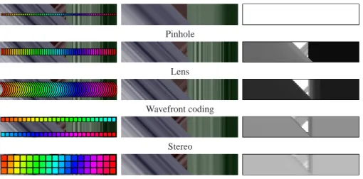
(a) Test image (b) light field and slope field (c) SSD error in reconstruction
Fig. 2.Light field reconstruction.
as the integral in eq5is intractable. We approximate the MAP estimate for the slope fieldS, and conditioning on this estimate, solve for the MAP light fieldx.
The slope field inference is essentially inferring the scene depth. Our inference generalizes MRF stereo algorithms [17] or the depth regularization of the coded aper-ture [1]. Details regarding slope inference are provided in [18], but as a brief summary, we model slope in local windows as constant or having one single discontinuity, and we then regularize the estimate using an MRF.
Given the estimated slope field S, our light field prior is Gaussian, and thus the MAP estimate for the light field is the mean of the conditional GaussianµS in eq6. This mean minimizes the projection error up to noise, and regularize the estimate by minimizing the oriented varianceΨS. Note that in traditional stereo formulations the multiple views are used only for depth estimation. In contrast, we seek a light field that satisfies the projection in all views. Thus, if each view includes aliasing, we obtain “super resolution”.
3.4 Empirical illustration of light field inference
Figure2(a,b) presents an image and a light field slice, involving depth discontinuities. Fig2(c) presents the numerical SSD estimation errors. Figure3presents the estimated light fields and (sparse samples from) the corresponding slope fields. See [18] for more results. Note that slope errors in the 2nd row often accompany ringing in the 1st row. We compare the results of the MOG light field prior with simpler Gaussian priors (ex-tending the conventional band limited signal assumptions [10,11,12]) and with modern sparse (but isotropic) derivative priors [19]. For the plenoptic camera we also explic-itly compare with signal processing reconstruction (last bar in fig2(c))- as explained in sec3.2this approach do not apply directly to any of the other cameras.
The prior is critical, and resolution is significantly reduced in the absence of a slope model. For example, if the plenoptic camera includes aliasing, figure 3(left) demon-strates that with our slope model we can super-resolve the measurements and the actual information encoded by the recorded plenoptic data is higher than that of the direct measurements.
The ranking of cameras also changes as a function of prior- while the plenoptic camera produced best results for the isotropic priors, a stereo camera achieves a higher
Plenoptic camera Stereo Coded Aperture
Fig. 3.Reconstructing a light field from projections. Top row: reconstruction with our MOG light field prior. Middle row: slope field (estimated with MOG prior), plotted over ground truth. Note slope changes at depth discontinuities. Bottom row: reconstruction with isotropic Gaussian prior
resolution under an MOG prior. Thus, our goal in the next section is to analytically evaluate the reconstruction accuracy of different cameras, and to understand how it is affected by the choice of prior.
4
Camera Evaluation Metric
We want to assess how well a light fieldx0can be recovered from a noisy projection y =T x0
+n, or, how much the projectionynails down the set of possible light field interpretations. The uncertainty can be measured by the expected reconstruction error:
E(|W(x−x0)|2;T) = Z
x
P(x|y;T)|W(x−x0)|2 (7)
whereW =diag(w)is a diagonal matrix specifying how much we care about different light field entries, as discussed in sec3.1.
Uncertainty computation To simplify eq7, recall that the average distance between x0
and the elements of a Gaussian is the distance from the center, plus the variance: E(|W(x−x0)|2|S;T) =|W(µS−x0)|2+
X
diag(W2ΣS) (8)
In a mixture model, the contribution of each component is weighted by its volume: E(|W(x−x0)|2;T) =
Z
S
P(S|y)E(|W(x−x0)|2|S;T) (9)
Since the integral in eq9 can not be computed explicitly, we evaluate cameras using synthetic light fields whose ground truth slope field is known, and evaluate an approxi-mate uncertainty in the vicinity of the true solution. We use a discrete set of slope field samples{S1, ...,SK}obtained as perturbations around the ground truth slope field. We
approximate eq9using a discrete average: E(|W(x−x0)|2;T)≈ 1
K
X
k
P(Sk|y)E(|W(x−x0)|2|Sk;T) (10)
Finally, we use a set of typical light fieldsx0
t (generated using ray tracing) and evaluate the quality of a cameraTas the expected squared error over these examples
E(T) =X t
Note that this solely measures information captured by the optics together with the prior, and omits the confounding effect of specific inference algorithms (like in sec3.4).
5
Tradeoffs in projection design
Which designs minimize the reconstruction error?Gaussian prior. We start by considering the isotropic Gaussian prior in eq 2. If the distribution of light fieldsxis Gaussian, we can integrate overxin eq11analytically to obtain:E(T) = 2Pdiag(1/η2
TTT +Ψ−1
0 )− 1
. Thus, we reach the classical PCA conclusion: to minimize the residual variance,T should measure the directions of max-imal variance inΨ0. Since the prior is shift invariant,Ψ−
1
0 is diagonal in the frequency domain, and the principal components are the lowest frequencies. Thus, an isotropic Gaussian prior agrees with the classical signal processing conclusion [10,11,12] - to sample the light field one should convolve with a low pass filter to meet the Nyquist limit and sample both the directional and spatial axis, as a plenoptic camera does. (if the depth in the scene is bounded, fewer directional samples can be used [10]). This is also consistent with our empirical prediction, as for the Gaussian prior, the plenop-tic camera achieved the lowest error in fig2(c). However, this sampling conclusion is conservative as the directional axis is clearly more redundant than the spatial one. The second order statistics captured by a Gaussian distribution do not capture the high order dependencies of light fields.
Mixture of Gaussian light field prior. We now turn to the MOG prior. While the
optimal projection under this prior cannot be predicted in closed-form, it can help us understand the major components influencing the performance of existing cameras. The score in eq9reveals two aspects which affect a camera quality - first, minimizing the varianceΣS of each of the mixture components (i.e., the ability to reliably recover the light field given the true slope field), and second, the need to identify depth and make P(S|y)peaked at the true slope field. Below, we elaborate on these components.
5.1 Conditional light field estimation – known depth
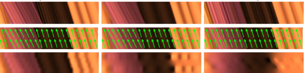
Fig 4shows light fields estimated by several cameras, assuming the true depth (and therefore slope field), was successfully estimated. We also display the variance of the estimated light field - the diagonal ofΣS (eq6).
In the right part of the light field, the lens reconstruction is sharp, since it averages rays emerging from a single object point. On the left, uncertainty is high, since it av-erages light rays from multiple points.In contrast, integrating over a parabolic curve (wavefront coding) achieves low uncertainties for both slopes, since a parabola “cov-ers” all slopes (see [18,20] for derivation). A pinhole also behaves identically at all depths, but it collects only a small amount of light and the uncertainty is high due to the small SNR. Finally, the uncertainty increases in stereo and plenoptic cameras due to the smaller number of spatial samples.
The central region of the light field demonstrates the utility of multiple viewpoint in the presence of occlusion boundaries. Occluded parts which are not measured properly
Pinhole
Lens
Wavefront coding
Stereo
Plenoptic
Fig. 4.Evaluating conditional uncertainty in light field estimate. Left: projection model. Middle: estimated light field. Right: variance in estimate (equal intensity scale used for all cameras). Note that while for visual clarity we plot perfect square samples, in our implementation samples were convolved with low pass filters to simulate realistic optics blur.
lead to higher variance. The variance in the occluded part is minimized by the plenoptic camera, the only one that spends measurements in this region of the light field.
Since we deal only with spatial resolution, our conclusions correspond to common sense, which is a good sanity check. However, they cannot be derived from a naive Gaussian model, which emphasizes the need for a prior such as as our new mixture model.
5.2 Depth estimation
Light field reconstruction involves slope (depth) estimation. Indeed, the error in eq9 also depends on the uncertainty in the slope fieldS. We need to makeP(S|y)peaked at the true slope fieldS0
. Since the observationyisT x+n, we want the distributions of projectionsT xto be as distinguishable as possible for different slope fieldsS. One way to achieve this is to make the projections corresponding to different slope fields concentrated within different subspaces of the N-dimensional space. For example, a stereo camera yields a linear constraint on the projection- theN/2samples from the first view should be a shifted version (according to slope) of the otherN/2. The coded aperture camera also imposes linear constraints: certain frequencies of the defocused signals are zero, and the location of these zeros shifts with depth [1].
To test this, we measure the probability of the true slope field, P(S0
|y), aver-aged over a set of test light fields (created with ray tracing). The stereo score is < P(S0
|y) >= 0.95(where< P(S0
|y) >= 1means perfect depth discrimination) compared to< P(S0
|y)>= 0.84for coded aperture. This suggests that the disparity constraint of stereo better distributes the projections corresponding to different slope fields than the zero frequency subspace in coded aperture.
We can also quantitatively compare stereo with depth from defocus (DFD) - two lenses with the same center of projection, focused at two different depths. As predicted by [21], with the same physical size (stereo baseline shift doesn’t exceed aperture width) both designs perform similarly, with DFD achieving< P(S0
|y)>= 0.92.
Our probabilistic treatment of depth estimation goes beyond linear subspace con-straints. For example, the average slope estimation score of a lens was< P(S0
|y)>= 0.74, indicating that, while weaker than stereo, a single monocular image captured with a standard lens contains some depth-from-defocus information as well. This result can-not be derived using a disjoint-subspace argument, but if the full probability is consid-ered, the Occam’s razor principle applies and the simpler explanation is preferred.
Finally, a pinhole camera-projection just slices a row out of the light field, and this slice is invariant to the light field slope. The parabola filter of a wavefront coding lens is also designed to be invariant to depth. Indeed, for these two cameras, the evaluated distributionP(S|y)in our model is uniform over slopes.
Again, these results are not surprising but they are obtained within a general frame-work that can qualitatively and quantitatively compare a variety of camera designs. While comparisons such as DFD vs. stereo have been conducted in the past [21], our framework encompasses a much broader family of cameras.
5.3 Light field estimation
In the previous section we gained intuition about the various parts of the expected error in eq9. We now use the overall formula to evaluate existing cameras, using a set of diffuse light field generated using ray tracing (described in [18]). Evaluated configura-tions include a pinhole camera, lens, stereo pair, depth-from-defocus (2 lenses focused at different depths), plenoptic camera, coded aperture cameras and a wavefront coding lens. Another advantage of our framework is that we can search for optimal parameters within each camera family, and our comparison is based on optimized parameters such as baseline length, aperture size and focus distance of the individual lens in a stereo pair, and various choices of codes for coded aperture cameras (details provided in [18]).
By changing the weights,W on light field entries in eq7, we evaluate cameras for two different goals: (a) Capturing a light field. (b) Achieving an all-focused image from a single view point (capturing a single row in the light field.)
We consider both a Gaussian and our new MOG prior. We consider different depth complexity as characterized by the amount of discontinuities. We use slopes between −45oto45oand noise with standard deviationη = 0.01. Additionally, [18] evaluates changes in the depth range and noise. Fig.5(a-b) plot expected reconstruction error with our MOG prior. Evaluation with a generic Gaussian prior is included in [18]. Source code for these simulations is available on the authors’ webpage.
Full light field reconstruction Fig.5(a) shows full light field reconstruction with our MOG prior. In the presence of depth discontinues, lowest light field reconstruction error is achieved with a stereo camera. While a plenoptic camera improves depth informa-tion our comparison suggests it may not pay for the large spatial resoluinforma-tion loss. Yet, as discussed in sec5.1a plenoptic camera offers an advantage in the presence of complex occlusion boundaries. For planar scenes (in which estimating depth is easy) the coded aperture surpasses stereo, since spatial resolution is doubled and the irregular sampling
1.5 2 2.5 3 3.5 4x 10 −3 pinhole lens wave front coding coded aperture DFDstereo plenoptic No depth discontinuities Modest depth discontinuities Many depth discontinuities
1 1.5 2 2.5x 10 −3 pinhole lens wave front coding coded aperture DFD stereo plenoptic No depth discontinuities Modest depth discontinuities Many depth discontinuities
(a) full light field (b) single view
Fig. 5.Camera evaluation. See [18] for enlarged plots
of light rays can avoid high frequencies losses due to defocus blur. While the perfor-mance of all cameras decreases when the depth complexity increases, a lens and coded aperture are much more sensitive than others. While the depth discrimination of DFD is similar to that of stereo (as discussed in sec5.2), its overall error is slightly higher since the wide apertures blur high frequencies.
The ranking in figs5(a) agrees with the empirical prediction in fig2(c). However, while fig5(a) measures inherent optics information, fig2(c) folds-in inference errors as well.
Single-image reconstruction For single row reconstruction (fig5(b)) one still has to account for issues like defocus, depth of field, signal to noise ratio and spatial resolution. A pinhole camera (recording this single row alone) is not ideal, and there is an advantage for wide apertures collecting more light (recording multiple light field rows) despite not being invariant to depth.
The parabola (wavefront coding) does not capture depth information and thus per-forms very poorly for light field estimation. However, fig5(b) suggests that for recov-ering a single light field row, this filter outperforms all other cameras. The reason is that since the filter is invariant to slope, a single central light field row can be recov-ered without knowledge of depth. For this central row, it actually achieves high signal to noise ratios for all depths, as demonstrated in figure4. To validate this observation, we have searched over a large set of lens curvatures, or light field integration curves, parameterized as splines fitted to 6 key points. This family includes both slope sensitive curves (in the spirit of [6] or a coded aperture), which identify slope and use it in the estimation, and slope invariant curves (like the parabola [5]), which estimate the cen-tral row regardless of slope. Our results show that, for the goal of recovering a single light field row, the wavefront-coding parabola outperforms all other configurations. This extends the arguments in previous wavefront coding publications which were derived using optics reasoning and focus on depth-invariant approaches. It also agrees with the motion domain analysis of [20], predicting that a parabolic integration curve provides an optimal signal to noise ratio.
5.4 Number of views for plenoptic sampling
As another way to compare the conclusions derived by classical signal processing ap-proaches with the ones derived from a proper light field prior, we follow [10] and ask: suppose we use a camera with a fixedN pixels resolution, how many different views (Npixels each) do we actually need for a good ‘virtual reality’?
0 10 20 30 40 0 1 2 3 4 5 6 7x 10 −3 Nyquist Limit Gaussian prior MOG prior
Fig. 6. Reconstruction error as a
function number of views. Figure6plots the expected reconstruction
er-ror as a function of the number of views for both MOG and naive Gaussian priors. While a Gaus-sian prior requires a dense sample, the MOG er-ror is quite low after 2-3 views (such conclu-sions depend on depth complexity and the range of views we wish to capture). For comparison, we also mark on the graph the significantly larger views number imposed by an exact Nyquist limit analysis, like [10]. Note that to simulate a re-alistic camera, our directional axis samples are aliased. This is slightly different from [10] which blur the directional axis in order to properly elim-inate frequencies above the Nyquist limit.
6
Discussion
The growing variety of computational camera designs calls for a unified way to ana-lyze their tradeoffs. We show that all cameras can be analytically modeled by a linear mapping of light rays to sensor elements. Thus, interpreting sensor measurements is the Bayesian inference problem of inverting the ray mapping. We show that a proper prior on light fields is critical for the successes of camera decoding. We analyze the limitations of traditional band-pass assumptions and suggest that a prior which explic-itly accounts for the elongated light field structure can significantly reduce sampling requirements.
Our Bayesian framework estimates both depth and image information, accounting for noise and decoding uncertainty. This provides a tool to compare computational cam-eras on a common baseline and provides a foundation for computational imaging. We conclude that for diffuse scenes, the wavefront coding cubic lens (and the parabola light field curve) is the optimal way to capture a scene from a single view point. For capturing a full light field, a stereo camera outperformed other tested configurations.
We have focused on providing a common ground for all designs, at the cost of sim-plifying optical and decoding aspects. This differs from traditional optics optimization tools such as Zemax that provide fine-grain comparisons between subtly-different de-signs (e.g. what if this spherical lens element is replaced by an aspherical one?). In contrast, we are interested in the comparison between families of imaging designs (e.g. stereo vs. plenoptic vs. coded aperture). We concentrate on measuring inherent informa-tion captured by the optics, and do not evaluate camera-specific decoding algorithms.
The conclusions from our analysis are well connected to reality. For example, it can predict the expected tradeoffs (which can not be derived using more naive light
field models) between aperture size, noise and spatial resolution discussed in sec5.1. It justifies the exact wavefront coding lens design derived using optics tools, and confirms the prediction of [21] relating stereo to depth from defocus.
Analytic camera evaluation tools may also permit the study of unexplored camera designs. One might develop new cameras by searching for linear projections that yield optimal light field inference, subject to physical implementation constraints. While the camera score is a very non-convex function of its physical characteristics, defining cam-era evaluation functions opens up these research directions.
Acknowledgments We thank Royal Dutch/Shell Group, NGA NEGI-1582-04-0004,
MURI Grant N00014-06-1-0734, NSF CAREER award 0447561. Fredo Durand ac-knowledges a Microsoft Research New Faculty Fellowship and a Sloan Fellowship.
References
1. Levin, A., Fergus, R., Durand, F., Freeman, W.: Image and depth from a conventional camera with a coded aperture. SIGGRAPH (2007)1,4,7,10
2. Veeraraghavan, A., Raskar, R., Agrawal, A., Mohan, A., Tumblin, J.: Dappled photogra-phy: Mask-enhanced cameras for heterodyned light fields and coded aperture refocusing. SIGGRAPH (2007) 1,4
3. Adelson, E.H., Wang, J.Y.A.: Single lens stereo with a plenoptic camera. PAMI (1992)1,4
4. Ng, R., Levoy, M., Bredif, M., Duval, G., Horowitz, M., Hanrahan, P.: Light field photog-raphy with a hand-held plenoptic camera. Stanford U. Tech Rep CSTR 2005-02 (2005) 1,
4
5. Bradburn, S., Dowski, E., Cathey, W.: Realizations of focus invariance in optical-digital systems with wavefront coding. Applied optics 36 (1997) 9157–91661,12
6. Dowski, E., Cathey, W.: Single-lens single-image incoherent passive-ranging systems. App Opt (1994) 1,12
7. Levoy, M., Hanrahan, P.M.: Light field rendering. In: SIGGRAPH. (1996)1,2
8. Goodman, J.W.: Introduction to Fourier Optics. McGraw-Hill Book Company (1968)1,2
9. Zemax:www.zemax.com.1,2
10. Chai, J., Tong, X., Chan, S., Shum, H.: Plenoptic sampling. SIGGRAPH (2000) 2,3,5,7,
9,13
11. Isaksen, A., McMillan, L., Gortler, S.J.: Dynamically reparameterized light fields. In: SIG-GRAPH. (2000) 2,3,5,7,9
12. Ng, R.: Fourier slice photography. SIGGRAPH (2005)2,3,5,7,9
13. Seitz, S., Kim, J.: The space of all stereo images. In: ICCV. (2001)2
14. Grossberg, M., Nayar, S.K.: The raxel imaging model and ray-based calibration. IJCV (2005)2
15. Kak, A.C., Slaney, M.: Principles of Computerized Tomographic Imaging.2
16. Baker, S., Kanade, T.: Limits on super-resolution and how to break them. PAMI (2002) 2
17. Scharstein, D., Szeliski, R.: A taxonomy and evaluation of dense two-frame stereo corre-spondence algorithms. Intl. J. Computer Vision 47(1) (April 2002) 7–423,7
18. Levin, A., Freeman, W., Durand, F.: Understanding camera trade-offs through a bayesian analysis of light field projections. MIT CSAIL TR 2008-049 (2008)4,7,9,11,12
19. Roth, S., Black, M.J.: Fields of experts: A framework for learning image priors. In: CVPR. (2005)5,7
20. Levin, A., Sand, P., Cho, T.S., Durand, F., Freeman, W.T.: Motion invariant photography. SIGGRAPH (2008) 9,12
21. Schechner, Y., Kiryati, N.: Depth from defocus vs. stereo: How different really are they. IJCV (2000) 11,14
![Fig. 5. Camera evaluation. See [18] for enlarged plots](https://thumb-us.123doks.com/thumbv2/123dok_us/365830.2540293/12.918.229.693.177.361/fig-camera-evaluation-enlarged-plots.webp)