Towards a Question Answering View of Natural Language Processing

(1)

Towards a Question Answering View of

Natural Language Processing

Submitted by

Andrej ˇ

Zukov-Gregoriˇc

for the degree of Doctor of Philosophy of the

Royal Holloway, University of London

(2)

Declaration

I, Andrej ˇZukov-Gregoriˇc, hereby declare that this thesis and the work presented in it is entirely my own. Where I have consulted the work of others, this is always clearly stated.

Signed . . . (Andrej ˇZukov-Gregoriˇc) Date:

(3)

(4)

Abstract

In recent years natural language processing research has tended to evolve through the successive modelling of various tasks. Examples include part-of-speech tagging, named entity recognition, co-reference resolution, various parsing tasks, language modelling, dialogue state tracking, extractive question answering (also called reading comprehen-sion), answer sentence selection, text summarization, machine translation, and even visual question answering. The goal of this thesis is threefold: to provide new architec-tures for a subset of the above; to propose a new model or task capable of generalising some of the above; finally, to build a dataset suitable for extractive question answering. We present results close to or above the state-of-the-art in named entity recognition (91.48 F1 on the CoNLL-2003 English dataset) and answer sentence selection (a 70.1% and 67.4% accuracy on the two test sets of InsuranceQA). Additionally, we provide a detailed ablation study of the well-known Bi-directional Attention Flow (BiDAF) model which we then use to suggest improvements to it. Finally, we introduce a new question answering dataset of labelled news data from armed-conflict events in the Iraq war.

(5)

Acknowledgement

I would like to thank my supervisor Zhiyuan Luo for initiating my interest in NLP. I started my PhD working on conformal prediction, followed by work on the probabilistic modelling of the spread of information across networks. I did not make much headway in these topics until I, by chance, was introduced to conditional random fields by Zhiyuan. This thesis is a testament to that moment. I would also like to thank our Department of Computer Science at Royal Holloway, as well as the Slovene Scholarship Fund for supporting me throughout my PhD.

In no particular order I would also like to thank my friends and colleagues: Dmitry Adamskiy, Sam Coope, Haotian Chen, Mayur Ladwa, Yoram Bachrach, Ed Tovall, Conan McMurtrie, Pasha Minkovsky, Attila Brozik, David Li, James Smith, Gre-gory Chockler, Jamie Alnasir, Michael Spagat, Florentyna Farghly, Pauline Heinrichs, Tim Scarfe, Han-Yi Chen, Ali Ahmed, Sam Robinson, ˇSpela Drnovˇsek-Zorko, Filip Drnovˇsek-Zorko, Joonas Karjaleinen, Raphael Reuben, Bryn Adams, Daniel Parting-ton, Sahil Wadhwa, Sebastian Janisch, Gabriel Hochstatter, Guy Doza, Nahom She-waybel, Sandford Sun, Maja Hakalo, Borjana Flipovska, Jasa Andrenˇsek, Luka Pilko, Volodya Vovk, James Smith, Asiana Jurca Avci and many, many, others for interesting technical conversations and for keeping me sane throughout my degree.

To my parents, Bojana and Miloˇs: none of this would have been possible without you. All your traits; your curiosity, your intellect, your strength and your love, you have selflessly, and through more sacrifice than most, given to me. For this, I am and forever will be, grateful.

(6)

2.2.2 Reading Comprehension . . . 27 2.2.3 Cloze-style Tasks . . . 29 2.3 Datasets . . . 30 2.3.1 CoNLL 2003 . . . 30 2.3.2 WikiQA . . . 31 2.3.3 InsuranceQA . . . 32 2.3.4 SQuAD . . . 32 2.3.5 IBC-C . . . 34 2.4 Evaluation . . . 34 2.4.1 Precision@k . . . 34 2.4.2 MRR . . . 34 2.4.3 F1 Score . . . 34

2.4.4 Micro and Macro Scores . . . 35

(7)

3 A Deep Learning Primer 36

3.1 Views of Language . . . 36

3.1.1 A Compositional View of Language . . . 36

3.1.2 A Sequential View of Language . . . 37

3.2 Recurrent Neural Networks . . . 38

3.2.1 Vanilla RNNs . . . 38 3.2.2 LSTMs . . . 38 3.2.3 Bi-directional RNNs . . . 39 3.2.4 Other architectures . . . 40 3.3 Attention Mechanisms . . . 40 3.3.1 Self-Attention . . . 41 3.3.2 Parametarized Attention . . . 41 3.3.3 Multi-head Attention . . . 41

3.4 Word and Sentence Representations . . . 41

3.4.1 Distributed Word Embeddings . . . 42

3.4.2 Sentence and Document Embeddings . . . 43

3.4.3 ELMo . . . 44

3.5 Siamese Networks . . . 44

3.6 Summary . . . 45

II Question Answering 46 4 A Detailed Ablation Study of the BiDAF Model 47 4.1 Introduction . . . 47

4.2 The BiDAF Model . . . 48

4.2.1 The Input Layers . . . 48

4.2.2 The Body Layers . . . 49

4.2.3 The Answer (Output) Layers . . . 51

4.2.4 Model Optimization . . . 52

4.3 Ablations . . . 54

4.3.1 Understanding Context2Query and Query2Context . . . 54

4.3.2 Uncompressed Query2Context Attention . . . 56

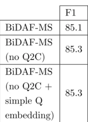
4.3.3 Using Different Question Representations . . . 57

4.3.4 Different Fusion Functions . . . 57

4.4 Multi-Span Answers . . . 58

4.4.1 Multilabel Loss . . . 58

(8)

4.4.3 Large Span Spaces . . . 59 4.4.4 A CoNLL QA dataset . . . 60 4.5 Results . . . 60 4.5.1 Ablation Results . . . 60 4.5.2 Multi-Span Results . . . 62 4.6 Implementation Details . . . 63 4.7 Related Work . . . 63 4.8 Summary . . . 64

5 A New NER Model 66 5.1 Introduction . . . 66

5.2 Named Entity Recognition . . . 66

5.2.1 LSTM complexity . . . 67

5.3 Parallel RNNs . . . 68

5.3.1 Promoting Diversity . . . 69

5.3.2 Output and Loss . . . 69

5.3.3 Relation to Ensemble Methods . . . 70

5.4 Results . . . 73

5.5 Implementation Details . . . 74

5.6 Related Work . . . 74

5.7 Summary . . . 75

6 A New Answer Selection Model 76 6.1 Introduction . . . 76

6.2 Preliminaries . . . 77

6.2.1 Embedding Questions and Answers . . . 79

6.2.2 Local Attention . . . 81

6.3 Global-Local Attention . . . 82

6.3.1 Creating Global Representations . . . 82

6.3.2 Combining Local and Global Representations to Determine At-tention Weights . . . 82

6.3.3 Building the Final Attention Based Representation . . . 84

6.3.4 Tuning Parameters to Minimize the Loss . . . 85

6.4 Results . . . 85

6.5 Implementation Details . . . 87

6.6 Related Work . . . 88

(9)

III A New Dataset 90

7 A New Dataset for Conflict Incident Question Answering 91

7.1 Introduction . . . 91

7.2 Creating the IBC-C Dataset . . . 92

7.2.1 Preprocessing . . . 92 7.2.2 Annotation . . . 93 7.2.3 Filtration . . . 94 7.2.4 Tasks . . . 96 7.2.5 Results . . . 102 7.3 Implementation Details . . . 103 7.4 Related Work . . . 103 7.5 Summary . . . 104 IV Conclusion 105 8 Conclusion and Future Work 106 8.1 Conclusion . . . 106

8.2 Future Work . . . 106

(10)

List of Figures

3.1 An example of a constituency parse tree. . . 37

3.2 An example of a dependency parse tree. . . 37

3.3 An LSTM network . . . 39

3.4 A bi-directional LSTM network . . . 39

3.5 The inside of an LSTM cell . . . 40

3.6 CBOW model . . . 43

3.7 Skip-gram model . . . 43

3.8 An example of a Siamese Network . . . 44

4.1 The BiDAF model. . . 53

5.1 A chart showing how multi-LSTM parameter complexity decreases as we shrink nand increase K. . . 67

5.2 An example of a parallel LSTM. FFNN is afeed-forward neural network. 68 6.1 Model architecture using answer-localized attention [133]. The left hand side used for the question. The right side of the architecture is used for both the answer and distractor. . . 78

6.2 Our proposed architecture with augmented attention. As in Figure 6.1, the right side of the model is used to embed answers and distractors. . . 78

6.3 A visualization of the attention weights for each word in a correct answer to a question. These examples show how the attention mechanism is focusing on relevant parts of the correct answer (although the attention is still quite noisy). . . 86

6.4 Performance of our system on InsuranceQA for various model sizes h (both the LSTM hidden layer size and embedding size) . . . 86

(11)

7.1 The IBC-C dataset visualised. A report is split into one or more non overlapping sections. A section is comprised of sentences which are com-prised of words. Each section is linked to exactly one incident which in turn can be linked to one or more sections. . . 92 7.2 A visualisation of the different steps taken to create the dataset. . . 94

(12)

List of Tables

2.1 Number of news articles, sentences, and tokens (words) in the

CoNLL-2003 English dataset. . . 30

2.2 Number of named entity types in the CoNLL-2003 English dataset. . . . 30

2.3 An example sentence from the CoNLL-2003 English dataset. . . 31

2.4 WikiQA dataset statistics. . . 31

2.5 WikiQA question type statistics. . . 31

2.6 An example question-answer pair from the WikiQA dataset. . . 32

2.7 InsuranceQA dataset statistics. . . 32

2.8 An example question-answer pair from the InsuranceQA dataset. . . 32

2.9 SQuAD dataset statistics. . . 33

2.10 SQuAD answer types. . . 33

2.11 An example taken from the SQuAD dataset. . . 33

4.1 CoNLL QA dataset statistics. . . 60

4.2 Existing BiDAF ablation results on the SQuAD dataset. [123] The Ex-act Match (EM) score measures the percentage of predictions that match any one of the ground truth answers exactly. . . 61

4.3 Our BiDAF ablation results on the SQuAD dataset. [123] . . . 61

4.4 CoNLL QA test set results using the BIDAF-MS multi-span model. . . 62

5.1 English NER F1 score of our model on the test set of CoNLL-2003 (En-glish). During training we optimize for the development set and report test set results for our best performing development set model. The bounded F1 results we report (±0.22) are taken after 10 runs. For the purpose of comparison, we also list F1 scores of previous top-performance systems. ‡ marks the neural models. ∗ marks model which use external resources. . . 71

(13)

5.2 Performance as a function of the number of RNN units with a fixed unit size of 64; averaged across 5 runs apart from the 16 unit model (averaged

across 10 runs). . . 71

5.3 Performance of our model with various unit sizes resulting in a fixed final output sizeht. Single runs apart from 16 unit. . . 72

5.4 Performance as a function of the unit size for our best performing model (16 biLSTM units). Single runs apart from with size 64. . . 72

5.5 Impact of various architectural decisions on our best performing model (16 biLSTM units, 64 unit size). Single runs. . . 72

6.1 Performance of various models on InsuranceQA . . . 87

7.1 An example of an incident hand coded by IBC staff. Min and max values represent the minimum and maximum figures quoted in report sections linked to the incident. . . 93

7.2 KSUB consideration rules . . . 95

7.3 ISUB consideration rules . . . 96

7.4 KNUM consideration rules. The hasOneTaggedAsKNUM column indi-cates whether the number ‘1’ is tagged as a KNUM (it could also be a pronoun). TheisKillSentence is determined by searching for kill-related keywords in the sentence. . . 97

7.5 INUM consideration rules . . . 98

7.6 LOCATION consideration rules . . . 99

7.7 DATE consideration rules . . . 99

7.8 WEAPON (usually the cause of death) consideration rules . . . 100

7.9 NER dataset statistics. Fully capitalized words indicate named entity tags. . . 100

(14)

List of Abbreviations

ACL Association of Computational Linguistics ADAM Adaptive Moment Estimation

AMTCL Association for Machine Translation and Computational Linguistics BiDAF Bi-Directional Attention Flow

BoW Bag of Words

CBOW Continuous Bag of Words CBT Children’s Book Test

CNN Convolutional Neural Network CRF Conditional Random Field

EM Exact Match

FPGA Field Programmable Gate Array GPU Graphics Processing Unit GRU Gated Recurrent Unit HMM Hidden Markov Model IBC Iraq Body Count IE Information Extraction IR Information Retrieval KB Knowledge Base

LSTM Long Short Term Memory

MUC Message Understanding Conference MRR Mean Reciprocal Rank

MT Machine Translation NER Named Entity Recognition NLP Natural Language Processing POS Part of Speech

QA Question Answering RNN Recurrent Neural Network

SEA Semantically Equivalent Adversary SQuAD Stanford Question Answering Dataset SVM Support Vector Machine

TF Term Frequency

(15)

Chapter 1

Introduction

Language is fundamentally inquisitive. Not only do we use it to convey information, we also use it to inquire for new information. Historically, most written text was of the former kind but with today’s popularity of messaging applications, we have seen an explosion in the amount of written data we have of the latter. This in turn has spurred research into question answering (QA) which is the study of models capable of answering questions across data.

Thenatural language processing (NLP) community divides question answering into two main categories depending on what the questions are being asked across. If across structured data, it is called structured QA, whereas if across unstructured data, it is calledtext QA. The two divisions have developed a separate focus.

Text QA research has focused heavily on attention models capable of detecting affinities between text and question. Much work has been done on detecting, mostly contiguous, answer spans in text. This has led to claims of human-level performance on certain well-known datasets. Recently however, there has been mounting evidence that suggests these models often learn to answer in a wrong way. They tend to focus on wrong parts of the question which makes them brittle in new contexts. There have been two main ways of remedying this. One has been through new datasets, the other through better inductive biases in the models themselves. Both strategies serve to help prevent models from learning spurious forms of reasoning.

Structured QA research has focused on two main data sources: knowledge bases (KBs) and tables. In the case of KBs, affinities between question and the contents of the KB (usually in the form of KB triplets) are modeled. Work on QA across tables on the other hand has seen attention from the neural semantic parsing community. Here, the mapping between question and logical form (such as a SQL query which then gets run across a table) is modeled. The logical form can be thought of as a blueprint for

(16)

1. Introduction

how to reason your way to the answer. Its generation can even be constrained to be both syntactically and semantically correct. However, it is unclear how this could be applied across unstructured data.

Many well known NLP tasks can be turned into a question answering task. For example, named entity recognition (NER) can be seen as a multi-span QA task. Sim-ilarly, much of information extraction (IE) can be seen as just QA across documents. Even seemingly unrelated tasks such as parsing can be thought of as questions answer-ing across text where the goal is to generate a parse. This unifyanswer-ing aspect of QA has helped open the door for the study of transfer and multi-task learning across differ-ent domains in NLP. For a long time NLP was forced to focus on small independdiffer-ent tasks; different models were developed and tailored for specific tasks like co-reference resolution, part-of-speech tagging, or constituency parsing. They were then pitted against each other on open datasets until they were “solved” only to have new, harder, datasets appear. Over time new datasets introduced harder and harder problems such as tasks involving dialogue or elements of computer vision. Concurrently, the unsu-pervised learning of word and sentence-level embeddings has armed downstream QA models with better inputs that have led to spikes in performance. Nevertheless, NLP is yet to have its ImageNet moment and although at least in question answering, the predominant mood now seems to be that of taking a step back and re-evaluating what it is our models are trying to learn.

All this, of course, matters, not only in and of itself, but also because of its use in application. Written questions nowadays appear in two main contexts: search and, more recently, dialogue (whether with an automated customer support agent or a home assistant). The proliferation of human-computer interaction is undoubtedly set to continue and the task of NLP research is to help equip it with ever better tools. This is not to say that the relationship between research and application is a one-way street, for surely it has been application which has over years heavily dictated the interests and directions of researchers in NLP. One need not look further than tasks which have preoccupied NLP for decades such as machine translation (MT) or more recent tasks such as . sentiment analysis, both driven by applicative need. In the former case, as a means of translating Cold War documents from Russian into English en masse; in the latter, as a way of predicting market sentiment in financial modeling or as a gauge of the quality of a product. Similarly, with question answering, it is clear that until we one day have fully automated customer service centers or home assistants with more human-like capabilities, applications such as these will continue to guide research in QA.

(17)

1.1. Contributions 1. Introduction

QA by focusing on three things: (1) the pitfalls of existing QA models, (2) entities and how they relate to QA, and (3) a new dataset created for QA across armed-conflict related texts. The thesis is divided into eight chapters and starts with chapter two where question answering, its history, and how it is viewed in linguistics is described. This is followed by a discussion of various different neural models used in the field in chapter three. The first substantive chapter with contributions is chapter four where we present a detailed ablation study of one of the most popular QA models and propose a new named entity QA task. Chapter five focuses on named entity recognition. Chapter six introduces a new answer selection model. Chapter seven introduces a new dataset for armed conflict analysis and presents results on it. Finally, chapter eight concludes this thesis with proposals for future work.

1.1

Contributions

The contributions in this thesis are contained in Chapters 4, 5, 6, and 7. We describe them briefly in turn:

Chapter 4

Chapter four presents an ablation study on the BiDAF reading comprehension model. We show that: (1) the model relies on its strong attention mechanisms to achieve good results (2) it is not sensitive to the complexity or simplicity of the question represen-tation (3) we propose a new form of attention which does not prematurely compress the question (4) we introduce a new dataset which combines reading comprehension with NER (5) we introduce an extension of the BiDAF model to the multi-span setting which we call BiDAF-MS.

Chapter 5

Chapter five introduces a new multi-LSTM model which is an end-to-end neural archi-tecture comprised of multiple ensemble-like bi-directional LSTMs. We show that our models achieves state of the art results on the CoNLL 2003 NER dataset.

Chapter 6

Chapter six focuses on another QA task called answer selection and introduces a new answer selection model which achieves state-of-the-art results on the InsuranceQA an-swer selection dataset. We achieve this by using a siamese architecture augmented with attention and a global view of the question and candidate answer.

(18)

1.2. List of Papers 1. Introduction

Chapter 7

Chapter seven introduces a new dataset of annotated armed-conflict news data. Using human-coded incident-level data about casualties in the ongoing conflict in Iraq we construct a base dataset which can be posited as either a NER, relationship extraction, event de-duplication, or question answering dataset.

1.2

List of Papers

The thesis is in part based on the following papers:

• Named Entity Recognition With Parallel Recurrent Neural Networks.

[39].

• An Attention Mechanism for Neural Answer Selection Using a Com-bined Global and Local View [7, 6].

• Neural Named Entity Recognition Using a Self-Attention Mechanism

[40].

(19)

Part I

(20)

Chapter 2

Question Answering

This chapter provides a thorough background on the topic of the thesis. The literature on this particular topic is huge, but we will try our best.

Question answering has a long history in both computing and natural language processing. This chapter begins by introducing the history behind question answering, followed by a review of what the areas of focus are today.

2.1

The History of Question Answering

Question can be thought of as utterances which we employ to retrieve information. Whether from or own memory or from some external context. As such, it is easy to see the central role question answering plays in natural language processing.

2.1.1 A brief history of NLP

Natural language processing is a very young field. We can trace its history back to the late 1940s. World War II had just ended and academia was spoiled for research directions to pursue. An entire generation of mathematicians, linguists, and engineers, on both sides, had just spent years contributing towards the war effort of their respec-tive sides. Many of them focused on code breaking and the machinery which made it feasible at scale - early computers. Code breakers developed a stable of techniques, runnable on the electromechanical or early electronic computers of the time or by so-calledhuman computers - groups of primarily women whose job it was to operate and program the computers as well hand-calculate or transcribe things when automated methods were found to be unfeasible. The code breaking techniques involved count-ing character, word, or n-gram frequencies; comparcount-ing documents; and through other

(21)

2.1. The History of Question Answering 2. Question Answering

over, questions naturally arose over whether the computers and techniques developed in code breaking could be applied to natural language instead of code.

This was a time of unprecedented international cooperation. International organi-zations such as the World Bank, the International Monetary Fund, the United Nations and its various agencies, had just been formed. The Nuremberg trials were ongoing, the Marshall plan was about to begin, and suspicions between the West and the So-viet Union festered. What a burning need, all of a sudden, to understand the world’s languages! And so, between roughly 1946 and 1949, Warren Weaver, a departmental director at the Rockefeller Foundation and a mathematician who had spent the war in operations research but who was familiar with communication theory and cryptogra-phy, began thinking about what would later become machine translation (MT). The result of his thoughts was a memorandum, entitledTranslation, which he completed in 1949. In it he cites a wonderful exchange between him and Norbert Wiener of MIT:

One thing I wanted to ask you about is this. A most serious problem, for UNESCO and for the constructive and peaceful future of the planet, is the problem of translation, as it unavoidably affects the communication between peoples. Huxley has recently told me that they are appalled by the magnitude and the importance of the translation job.

Recognizing fully, even though necessarily vaguely, the semantic difficulties because of multiple meanings, etc., I have wondered if it were unthinkable to design a computer which would translate. Even if it would translate only scientific material (where the semantic difficulties are very notably less), and even if it did produce an inelegant (but intelligible) result, it would seem to me worth while.

Also knowing nothing official about, but having guessed and inferred con-siderable about, powerful new mechanized methods in cryptographymethods which I believe succeed even when one does not know what language has been codedone naturally wonders if the problem of translation could conceivably be treated as a problem in cryptography. When I look at an article in Rus-sian, I say: ”This is really written in English, but it has been coded in some strange symbols. I will now proceed to decode.”

Have you ever thought about this? As a linguist and expert on computers, do you think it is worth thinking about?

(22)

Second - as to the problem of mechanical translation, I frankly am afraid the boundaries of words in different languages are too vague and the emo-tional and internaemo-tional connotations are too extensive to make any quasi-mechanical translation scheme very hopeful. I will admit that basic English seems to indicate that we can go further than we have generally done in the mechanization of speech, but you must remember that in certain respects basic English is the reverse of mechanical and throws upon words a burden which is much greater than most words carry in conventional English. At the present time, the mechanization of language, beyond such a stage as the design of photoelectric reading opportunities for the blind, seems very premature. . . .

Despite not having convinced Wiener, Weaver convinced many others including policy makers which responded with plentiful funds to fund research into the topic. In tandem with Weaver, disparate efforts elsewhere were ongoing. In particular, Andrew D. Booth of Birkbeck College and Richard H. Richens (a botanist turned computational linguist) of the Commonwealth Bureau of Plant Breeding and Genetics were by then working on a mechanized dictionary capable of translating individual words using a rule-based method. Similar efforts were being worked on, on one of the computers in California.

Research into machine translation soon opened other areas of focus which needed to be addressed such as syntactics and semantics. From this, new grammars, parsers, and what today we would call lexical databases were created. As these sub-problems turned into sub-fields, modern NLP slowly began to be born. In 1954 the ability to translate simple technical Russian into English was showcased in the IBM-Georgetown demonstration. In 1962 the Association for Machine Translation and Computational Linguistics (AMTCL) was formed - later to be renamed to today’s well known Associ-ation for ComputAssoci-ational Linguistics (ACL) in 1968.

Progress in MT was nevertheless slow. Despite early optimism that machine trans-lations would be solved within years, the end was nowhere in sight. In 1964 the US government set up the Automatic Language Processing Advisory Committee. Their task: to evaluate progress in machine translation and computational linguistics. Their 1966 report titledComputers in Translation and Linguistics was critical of the progress achieved and as a result funding for MT was heavily curtailed. The report emphasized the need for more basic research in computational linguistics and as a result NLP became more diversified.

(23)

knowl-2.1. The History of Question Answering 2. Question Answering

edge bases. Lexical databases such as WordNet and other knowledge bases based on semantic frames, were developed. Work in these areas complemented and intersected with work being done on expert systems. This was the era of great optimism that soft-ware systems could help humans solve tasks faster. Systems exposed natural language interfaces to be able to query structured data. SHRDLU (1970) could answer ques-tions and enact prompts in a simple block world; PARRY (1972) was an early chatbot which attempted to simulate a person with paranoid schizophrenia; KL-ONE (1974) reasoned across knowledge bases, SAM (1975) and PAM (1978) understood stories and could launch procedures as a result or answer questions about them. These systems in turn spurred research into more basic NLP research such as statistical parsing, part-of-speech tagging POS tagging, knowledge-base creation, and intent recognition.

In the early 1980s it was hoped that natural language interfaces would be the de facto way of interfacing with computers (instead of having to type complicated commands into the terminal). Entire companies such as Symantec were founded on this premise. Instead, with the advent of GUI operating systems (Mac OS 1.0 in 1984 quickly followed by Windows 1.0 and AmigaOS 1.0 in 1985), curtailed research into expert systems and natural language interfaces.

Running in parallel with the work being done on the above, research into the sta-tistical analysis of language started gaining traction. Hidden Markov models, which had been developed in the late 1950s and throughout the 1960s by the likes of Rus-lan Stratonovich and Leonard E. Baum (known for the Baum-Welch algorithm), saw their application first in speech recognition and later in tasks which could be posited as sequence classification problems such as POS tagging and eventuallynamed entity recognition (NER).

The 1990s saw an explosion in statistical NLP methods as the machine learning and NLP communities edged ever closer. Structuredsupport vector machines (SVMs), conditional random fields(CRFs), recurrent neural networks (RNNs)1 all started to be applied to language by the end of the decade. The standardization and proliferation of NLP tasks allowed the community to more easily compete on solving them. Conferences such as the first Text Retrieval Conference (TREC, 1992), SemEval-1 (1998), and Conll-1999, promoted shared tasks which saw researchers around the world compete on information retrieval (IR) and computational semantics analysis tasks.

The 2000s saw a maturing of these methods as researchers focused on an ever-growing list of shared tasks, various flavors of models, and perhaps what looking back would mark the decade - hand-engineered features. By the end of the decade, intri-cate models, compliintri-cated pipeline systems, and baroque hand-engineered features had

(24)

achieved measurable progress in most tasks. Simple tasks such as POS tagging and NER were considered close to being solved and much progress had been made on tasks such as co-reference resolution, semantic role labeling, word sense disambiguation, and sentiment analysis. Important caveats where the then state-of-the-art models failed remained. Pointedly, the way this was tackled was usually by adding more and better hand-engineered features.

An important shift happened in the early 2010s with a few key incursions of deep learning into the field. Distributed word representations in vector space appeared in 20112and were shown to substantially improve the performance of downstream models. As a direct result of this research, study into distributed word vector space models has blossomed and researchers are now trying to encode as much information into word embeddings as possible. In 2012 the now widely used sequence-to-sequence model was developed, immediately improving results in machine translation and semantic parsing. It was in the 2010s that mobile phones went from being devices used to call and text people to so-called smartphones - devices with which users could book flights, bank, check cycle routes, video call, book a cab, and, towards the end of the decade, even begin to use as smart personal assistants. Despite it being easier than ever before to place a call, smart phones users in the 2010s turned unexpectedly to messaging each other. This has reignited hopes that natural language, whether through voice or text, could again be used to interface with complex systems. As a result, study into dialogue systems saw increased interest, as did some of its sub-tasks, including semantic parsing and question answering.

At the time of writing it is late 2018 and we are slowly edging towards the end of another decade. Looking forward we can probably expect work in the next decade to continue to push the boundaries of deep learning NLP models. We can expect to see word and sentence or document level embedding models to mature as we find better ways of encoding information in them. This will lead to significant improvements in downstream tasks. Just as in the computer vision community, we are beginning to see more attention being paid to the robustness of our models and their brittleness to adversarial examples. Dialogue systems will improve as households acquire smart home assistants en masse, as a result we can expect continued interest in dialogue state tracking, question answering, and semantic parsing. A tougher nut to crack will be problems which we have only skirted the surface of such as true transfer learning and how memories are stored, retrieved, and used.

And what of machine translation? The original problem which helped spark

re-2

The first such models was actually introduced by Rumelhart, Hinton, and Williams in 1986 but distributed word representations first really saw their use in the early 2010s.

(25)

search into what would become modern NLP? As of 2018, the strongest neural machine translations systems perform close to par with humans.

2.1.2 A brief history of QA

Question answering traces its history back to the early days of NLP. From the very beginning there was a distinction betweenstructured QAandtext QA. The two branches distinguished themselves not only by the types of data questions were asked across but also by their application. Structured QA was seen as a means of providing an interface to complex structured data whereas text QA was initially seen as a frontend toinformation retrieval. Later, text QA would become an object of separate study as part ofreading comprehension.

In 1961 researchers at MIT revealed BASEBALL [38], a system capable of auto-matically answering questions across a structured baseball dataset. Its introduction confidently stated that:

Men typically communicate with computers in a variety of artificial, styl-ized, unambiguous languages that are better adapted to the machine than to the man. For convenience and speed, many future computer-centered systems will require men to communicate with computers in natural lan-guage. The business executive, the military commander, and the scientist need to ask questions of the computer in ordinary English, and to have the computer answer questions directly. Baseball is a first step toward this goal.

In 1965 a survey by Simmon et al. [128] mentioned no fewer than fifteen English language QA systems built over the preceding five years including early conversational agents. In the mid 1970s work by Wendy Lehnert influenced by Roger Schank and conceptual dependency theory introducedQUALM [74], a question answering program capable of answering questions about text. It was later used as a part of theSAM and PAM story understanding systems. Lehnert was one of the first NLP researchers to focus ontext QAas an area of independent study. QUALM worked by first classifying the question into one of thirteen conceptual categories before using heuristics to find the answer.

Despite having studied text QA in situ, QUALM failed to spark research into the new field. Perhaps one of the most decisive reasons for this was the lack of a stan-dardized dataset, or task, to help research coalesce around a shared goal. This at last happened with the inclusion of a QA task into the 1999 Text Retrieval Conference

(26)

2.2. Question Answering Research Today 2. Question Answering

(TREC) [139] where the task was to retrieve a ranked list of five documents and cor-responding answer snippets (short passage of text which contain the answer). As a result, research into QA has continued to blossom over the past 20 years.

Initially, researchers used pipeline approaches to try and tackle these new shared QA tasks. A common pipeline was:

1. Question Analysisquestions would first be analyzed and classified as belonging to a particular type using either heuristics or through some machine learning method (see [78]).

2. Candidate Document Selection A limited subset of candidate documents believed to contain the answer would be selected.

3. Answer ExtractionItems at varying granularities depending on the task would be ranked or classified in terms of their probability of containing the answer. Items here could range from the individual documents themselves down to sub-strings of the documents, individual sentences, or even short sequences of words.

4. Response GenerationAn appropriate response to be returned to the user was generated or selected.

With continued adoption of statistical and later deep learning methods in NLP the above pipeline began shedding heuristics and adopting a more end-to-end approach.

In what follows we cover some of the recent work done in the various sub-tasks of QA that have matured over the past two decades with a special focus on reading comprehension and sentence selection - the two main topics of this thesis.

2.2

Question Answering Research Today

Question answering, just like the rest of NLP research today, slots almost wholly within the prevailing deep learning paradigm. Deep learning methods have consis-tently achieved state-of-the-art results in the field and progress has been rapid.

The reason behind the move in NLP from the more traditional, statistical, ap-proaches to deep learning is for the most part because deep learning methods allow for the more expressive modelling of textual inputs and as a result have achieved much better results on NLP tasks. As an example, modeling the long and short distance sequential dependencies in variable length text is a lot easier to achieve using recurrent neural networks than more traditional approaches which would have either disregarded these dependencies or modelled them using models not as expressive or as general as

(27)

2.2.1 Open-Domain Question Answering and Sentence Selection

Open-domain QA is the task of finding answers in collections of unstructured docu-ments. Today, it roughly corresponds to steps 2. and 3. of the previous section. With emphasis on the lots of documents! It is the most closely related sub-field of QA with information extraction and as such also closely related to some of the technology under-pinning modern search engines. It is also the branch of QA championed by TREC-QA between 1999 and 2007. The emphasis was always on having to handle large numbers of documents which makes it a great problem to think of in terms of learning to rank all the documents. In 2007, the now somewhat confusingly named TrecQA, or sometimes QASent, dataset was created using some of the original TREC data. It contained a total of 227 questions and 8,478 candidate answers. Significantly, the dataset contained only question-answer pairs with overlapping words.

Recently, research has coalesced around a number of frequently used datasets which try to address some of the deficiencies observed in the original TREC data.

WikiQA [150], released in 2015, is an order of magnitude larger than the datasets released by TREC-QA and focuses on the candidate document selection step (now more commonly called sentence selection or answer selection) from a set of pre-selected sentences. A total of 3,047 questions and 29,258 candidate answer sentences are col-lected from Bing search queries and Wikipedia summaries respectively. Notably, some questions do not have any corresponding correct answer sentences. Further, unlike many instances in TREC, WikiQA data significantly reduces the bias towards lexical overlap (shared words) between question and candidate answer text.

InsuranceQA [26], also released in 2015, expanded the size of sentence selection datasets again this time including many more questions (17,487) and a comparable number of candidate answers (24,981). Released by IBM, the dataset is noteworthy for focusing on a single domain - insurance - using actual questions searched for by users and featuring answers written by experts. Put otherwise, the dataset came from a real-world use case.

Finally, the SemEval-2016 cQA challenge [30], introduced three selection sub-tasks: (1)question-comment similarity where the task is to rank the comments left beneath a question according to their relevance (2)question-question similarity where the task is to rank a question to a set of other related questions according to their similarity, and (3) question-external comment similarity where the task is to, given a new question, rank the 100 comments associated with the 10 most related questions to the new question.

The above datasets have all contributed towards a range of deep learning models which divide roughly into three architectural categories:

(28)

• Siamese Architectures. First introduced in 1993 by [13], siamese networks work by encoding input into embeddings using the same encoder before comparing the embeddings using some scoring function. The idea is to make the model score correct question-candidate pairs above wrong (so called distractor) pairs by learning an encoder which brings correct pair embeddings closer together in space. Recent examples include the non-attentive model in [134] as well as [108], [44] which even outperform some attentive architectures.

• Attentive Architectures. Learning an encoder function can be hard. To make the computation of an embedding more dependent on other inputs, we may attend across them. Attention mechanisms were first described in 2014 in [8] and have seen wide adoption in NLP since. Recent works on answer selection include the attentive model in [134] and the work by [117].

• Compare-Aggregate Architectures. The motivation behind compare-aggregate architectures is to delay the aggregation into embeddings to occur as late as possi-ble and to compare as much as possipossi-ble along the way. Each contextual represen-tation of one input (such as a word) is compare to all contextual represenrepresen-tations of the other input thus forming an outer product matrix of representation com-parisons. These are then reasoned across using various aggregation steps thus allowing for more fine-grained inter-dependence than with normal attentive ar-chitectures. There has been a lot of work very recently on these types of models including initially in work by [45] followed by [144] and [136].

An excellent review of the above methods can be found in [69].

2.2.2 Reading Comprehension

Reading comprehension is the task of reasoning across, usually a single passage, of unstructured text to answer a question. The answer can either be a (1) span extracted from the passage (2) a set of multiple extracted spans (3) an answer picked from a set of multi-choice candidate answers, or (4) generated.

The history of modern reading comprehension dates back to Hirschmann et al. [51] and their work on - the fashionably named -DEEP READ, an automated reading com-prehension system which learned to find the sentence containing the right answer using a combination of heuristic pattern-matching techniques on hand-engineered features. The data their system was tested against comprised of easy to understand simulated news stories with associated questions of a 3rd-6th grade comprehension difficulty. The system was tested on a small development set made up of 60 passages and applied on a

(29)

similarly sized test set. Each passage was associated with 5 questions giving a total of 600 questions. DEEP READ could identify the sentence containing the correct answer 30-40% of the time. These scores were later to be improved on by others. A year later Ng et al. [95] published the first statistical model (logistic regression) to be used on the dataset achieving results competitive with previous heuristic approaches (this was still a time in NLP when it wasn’t clear whether statistical approaches would prevail). New datasets much like the above were released throughout the 2000s, Breck et al. [12] released 75 stories from the Canadian Broadcasting Corporation’s website together with 650 associated questions. This data was then enriched in 2003 by Leidner et al. [75]. On the modelling side, efforts remained much the same and were either heuristics or simple machine learning methods (both of which used hand-engineered features as input).

With increased computational power and the adoption of deep learning methods in NLP towards the end of the 2000s came the need for new datasets and new models. MCTest [114], released in 2013, contains 500 stories and 2000 questions and is a multi-choice reading comprehension task with 4 candidate answers per question.

Neural models continued to struggle on reading comprehension tasks and the best of models only recently began to perform on-par with the best handcrafted ones. Notably, [138] presented at ACL 2016, was the first neural model to outperform handcrafted ones on MCTest by a small margin.

2016 was also the year in which theStanford question answering dataset (SQuAD) was released. Considered somewhat of a watershed moment for reading comprehension, it catapulted reading comprehension into the limelight and there have been over 70 proposed models which have been submitted to its leader board where models compete against one another. Version 1.1 of the dataset contained over 100,000 questions and 536 passages of (so called) context text. The recently released version 2.0 of the dataset [104] adds unanswerable questions into the mix.

The vast majority of SQuAD models are very similar. Roughly speaking they all divide into three layers:

• Input Layer. The input layer’s responsibility is to take input representations (usually of words, or characters) and transform them into contextual embeddings which better represent the input passage and question. A very common approach is to combine pre-trained word embeddings with character-level embeddings by appending the output of an LSTM or CNN across the characters which make up the corresponding word embeddings. The combined word-character embeddings are then passed through an LSTM to contextualize them. We are left with a sequence of embeddings of the same length as the context (or question depending

(30)

on what is being embedded) which contain information about their surrounding context and thus represent the inputs better.

• Body Layer. The body layer is where reading comprehension models model the dependencies between passage and question. This is done through various atten-tion steps using attenatten-tion, co-attenatten-tion and/or self-attenatten-tion modules. Notable examples include BiDAF [123], Dynamic CoAttention Networks [148], Stochas-tic Answer Networks [80], QANet [151], FusionNet [55]. We explore BiDAF in greater detail in a subsequent chapter.

• Answer Layer. The answer layer takes the outputs of the body layer and converts them into predictions. Predictions in reading comprehension come in two main flavours: (1) span predictions; where the goal is to predict one or more spans of passage text by either predicting the start and end index (or indexes) or by enumerating across all spans in order to classify across them or classify each one of them or (2) generative predictions; where the goal is to generate the correct answer.

Since SQuAD 1.0’s release there has been work criticizing the dissecting the dataset’s structure and the models which compete on it. My work on analyzing BiDAF can be looked at in this vein. Three recent works stand out here. Jia and Lang (2017) [58] show that simple adversarial examples such as adding extra characters to questions can successfully trick models. Even more recently, [113] formalize adversarial examples for reading comprehension through their semantically equivalent adversarial examples framework which shows that models perform poorly on simple paraphrases. Finally, [141] perform a comparative error study of various reading comprehension models on SQuAD.

Another popular machine comprehension dataset which has seen continuing focus recently is the set of bAbI tasks [147] originally introduced in 2015 and since expanded. Whereas SQuAD tries to cover as broad of a set of topics and questions as possible and to make sure that all text is human generated, bAbI on the other hand is a synthetic dataset with a focus of exploring how comprehension models perform on simple well structured synthetic datasets allowing researchers to see where specifically these models fail.

2.2.3 Cloze-style Tasks

Cloze-style datasets, where the the goal is to predict the missing word in a passage of text, have become a popular way of automatically generating large reading

(31)

compre-2.3. Datasets 2. Question Answering

The most popular dataset in the field is the Children’s Book Test (CBT) [49] where the goal is to predict a blanked-out word of a sentence given 20 previous sentences. Other examples include the cloze-style CNN / Daily Mail corpus created by [46]. However, as discussed in [105], it is difficult to create hard cloze-style datasets because the blanked out words are usually entities or single words which are heavily dependent on a short context.

2.3

Datasets

In this section, I describe in more detail the datasests used in the thesis.

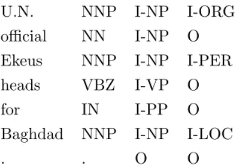
2.3.1 CoNLL 2003

The CoNLL 2003 NER shared task dataset [137] is a collection sentences where each word is assigned an entity label which identifies it as a organization,person, location, or as miscellaneous. The task is most commonly posited as a sequence labelling task. Traditionally, models such as HMMs and CRFs would have been used to solve this task but more recently, research has focused on studying the performance of various recurrent neural architectures.

.

English data Articles Sentences Tokens Training set 946 14,987 203,621 Development set 216 3,466 51,362

Test set 231 3,684 46,435

Table 2.1: Number of news articles, sentences, and tokens (words) in the CoNLL-2003 English dataset.

English data LOC MISC ORG PER Training set 7140 3438 6321 6600 Development set 1837 922 1341 1842 Test set 1668 702 1661 1617

Table 2.2: Number of named entity types in the CoNLL-2003 English dataset.

(32)

2.3. Datasets 2. Question Answering

U.N. NNP I-NP I-ORG official NN I-NP O Ekeus NNP I-NP I-PER heads VBZ I-VP O

for IN I-PP O

Baghdad NNP I-NP I-LOC

. . O O

Table 2.3: An example sentence from the CoNLL-2003 English dataset.

2.3.2 WikiQA

The WikiQA dataset is an early answer selection dataset [150]. The task is to classify or learn to rank across a number of candidate answers given a question. Questions are usually short, whereas candidate answers are usually multi-sentence paragraphs. In the case of WikiQA, the former are human-coded whereas the latter are collected from Wikipedia.

Train Dev Test Total Questions 2,118 296 633 3,047 Sentences 20,360 2,733 6,165 29,258

Answers 1,040 140 293 1,473

Average ques. length 7.16 7.23 7.26 7.18 Average sent. length 25.29 24.59 24.95 25.15 Questions w/o ans. 1,245 170 390 1,805

Table 2.4: WikiQA dataset statistics.

Question type Counts % Location 373 12 Human 494 16 Numeric 658 22 Abbreviation 16 1 Entity 419 14 Description 1,087 36

(33)

Question Who wrote second Corinthians?

Answer

Second Epistle to the CorinthiansThe Second Epistle to the Corinthians, often referred to as Second Corinthians (and written as 2 Corinthians),

is the eighth book of the New Testament of the Bible. Paul the Apostle and Timothy our brother wrote this epistle to the church of God which is at Corinth, with all the saints which are in all Achaia.

Table 2.6: An example question-answer pair from the WikiQA dataset.

2.3.3 InsuranceQA

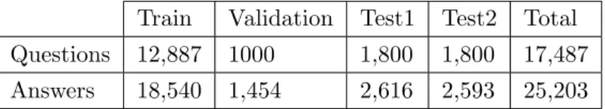
Similar to WikiQA, InsuranceQA is an answer selection dataset where answers must be classified across or ranked [26].

Train Validation Test1 Test2 Total Questions 12,887 1000 1,800 1,800 17,487 Answers 18,540 1,454 2,616 2,593 25,203

Table 2.7: InsuranceQA dataset statistics.

Question Does Medicare cover my spouse?

Answer

If your spouse has worked

and paid Medicare taxes for the entire required 40 quarters, or is eligible for Medicare by virtue of being disabled or some other reason, your spouse can receive his/her own medicare benefits. If your spouse has not met those qualifications, if you have met them, and if your spouse is age 65, he/she can receive Medicare based on your eligibility.

Table 2.8: An example question-answer pair from the Insur-anceQA dataset.

2.3.4 SQuAD

The Stanford Question Answering Dataset [105] is a machine reading comprehension dataset where the task is to find the correct answer span of words in thecontext text given aquestion. In the case of SQuAD, there is only ever one correct answer span in

(34)

everycontext-question pair and it is always contiguous (i.e. a sequence of neighbouring words).

Train Validation Test (hidden) Question-answer pairs 87,599 10,570 9,616

Articles 442 48 46

Context paragraphs 18,891 2,067 2,257

Table 2.9: SQuAD dataset statistics.

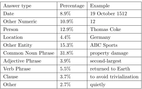
Answer type Percentage Example

Date 8.9% 19 October 1512

Other Numeric 10.9% 12

Person 12.9% Thomas Coke

Location 4.4% Germany

Other Entity 15.3% ABC Sports Common Noun Phrase 31.8% property damage Adjective Phrase 3.9% second-largest Verb Phrase 5.5% returned to Earth Clause 3.7% to avoid trivialization

Other 2.7% quietly

Table 2.10: SQuAD answer types.

Context paragraph Nikola Tesla (Serbian Cyrillic: ; 10 July 1856 7 January 1943) was a Serbian American inven-tor, electrical engineer, mechani-cal engineer, physicist, and futur-ist best known for his contribu-tions to the design of the modern alternating current (AC) electric-ity supply system.

Question What does AC stand for? Answer alternating current

(35)

2.4. Evaluation 2. Question Answering

2.3.5 IBC-C

Please see Chapter 7 for a further description of IBC-C.

2.4

Evaluation

A few common evaluation metrics are used throughout this thesis. We briefly go over them here.

2.4.1 Precision@k

Precision atk(often denoted asp@k) corresponds to the number of relevant results in the k retrieved results. As a result, p@1 can be thought of as accuracy whereas, for example, p@5 is the ratio of times the correct answer appears in the top 5 retrieved results. We use p@kas a measure of accuracy in answer selection.

2.4.2 MRR

Mean reciprocal rank (MRR) is another metric used to score retrieval models. Retrieval models (including answer selection models which learn to rank) output a sorted list of predictions. The rank is the index of the first correct answer to appear in that list. Thereciprocal rank is just the rank−1. And themean reciprocal rank is just the mean of reciprocal ranks.

For example, in a test set made up of three examples where our model ranked the correct answers as 1,3,6; thereciprocal ranks would be 1,1₃,1₆ and the MRR would be

1 2 MRR = 1 |Q| |Q| X i=1 1 ranki (2.1) 2.4.3 F1 Score

The F1 score is defined as the harmonic mean of precision and recall:

F1 = recall−1+ precision−1 2 −1 = 2· precision · recall precision + recall (2.2) It is probably the single most used metric in NLP. The motivation behind that is that it takes a look at both the recall and precision of a model and not just the accuracy. In cases where there are class imbalances, the discrepancy between the two can be very large and accuracy results can be misleading.

(36)

2.5. Summary 2. Question Answering

2.4.4 Micro and Macro Scores

Micro- and macro-score on any of the above metrics will compute two different things. A macro-average will compute the metric independently for each class and then take the average (hence treating all classes equally), whereas a micro-average will aggregate the contributions of all classes, before computing the average score.

2.5

Summary

We have now reviewed the history of question answering and how it fits in the wider NLP context. Further, we have gone over some of the most recent research in question answering. Finally, we introduce the datasets used in this thesis. In the next chapter we will look at our first question answering model.

(37)

Chapter 3

A Deep Learning Primer

This chapter provides yet more background information.

3.1

Views of Language

3.1.1 A Compositional View of Language

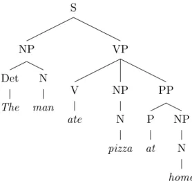
It is generally agreed that language is compositional and follows a hierarchy ranging from words and characters to clauses, sentences, and entire documents - the under-standing any of which might even be dependent upon knowledge of some external context. Linguists and NLP researchers have long explicitly modelled the composi-tional structure of language. Perhaps the two best examples of this are constituency and dependency parses of sentences (Figure 3.1 and Figure 3.2, respectively).

Parses of language model it as being made up of terminals (words) and non-terminals(in the case of Figure 3.1 Penn Treebank tags) which can operate on terminals or on other non-terminals themselves. Work on recursive neural nets which function across such parse trees (as popularized [129])has been a promising recent avenue of research but has been hampered by the difficulty of efficiently training such neural architectures.

(38)

3.1. Views of Language 3. A Deep Learning Primer S NP Det The N man VP V ate NP N pizza PP P at NP N home

Figure 3.1: An example of a constituency parse tree.

A hearing is scheduled on the issue today . ROOT ATT ATT SBJ PU VC TMP PC ATT

Figure 3.2: An example of a dependency parse tree.

3.1.2 A Sequential View of Language

Another way of looking at language is just as a sequence of words. The task is then to model language using models capable of reasoning across sequences. This view on language traces its history back to early sequential models such as hidden Markov models and conditional random fields. In deep learning, the most popular models have become recurrent neural networks starting with vanilla RNNs, followed by LSTMs, GRUs, and other recurrent neural network variants.

The sequential modelling of language does not fully ignore the compositional view, but instead, models it implicitly and argues that its explicit modelling is unnecessary. This thesis follows the sequential view of language.

(39)

3.2. Recurrent Neural Networks 3. A Deep Learning Primer

3.2

Recurrent Neural Networks

Recurrent neural network architectures are a family of neural architectures capable of handling sequntial input. Their names originate from the recurrent application of the same set of parameters at each time-step and their dependence at each time-step on not only the present input but also the networks previous state.

3.2.1 Vanilla RNNs

The simplest form of recurrent neural network is the vanilla RNN shown here:

ht=σ(Whht−1+Wixt+bh)

ot=σ(Woht+bo)

(3.1)

Where Wi, Wh and Wo are the input, recurrence, and output parameters; bh and

bo the bias terms; ht the hidden states (or network states); and, xt and ot the inputs

and outputs. Notice that one canunroll the above across time-steps and think of it as a deep feed-forward neural network where inputs are fed to it at every layer.

The problem with the above vanilla RNN model is that it comes with a set of deficiencies which make it hard to train. Above all else, the above model is unstable because during optimization, its gradients may explore or vanish. It is easy to intu-itively see why that is. Thinking of Equation 3.1 in its unrolled form and taking its derivative with respect to any of its parameters it is easy to see how one must borough through the function using the chain rule. This leads to a product of Jacobians as the derivative passes through the hidden layers. Just as the product of numbers just smaller than 1 collapse to 0 and just above 1 explode to infinity, so too do the gra-dients of vanilla RNNs behave. There are many hacks which to varying degrees solve this problem, such as clipping the gradients if they pass a certain threshold, but there has been much research since on architectures which do not experience this problem.

3.2.2 LSTMs

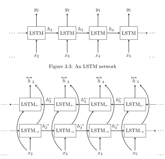
Motivated by the exploding and vanishing gradients problems of vanilla RNNs, long-short term memory networks (LSTMs) were invented as a result.

ft=σg(Wfxt+Ufht−1+bf) it=σg(Wixt+Uiht−1+bi) ot=σg(Woxt+Uoht−1+bo) ct=ft◦ct−1+it◦σc(Wcxt+Ucht−1+bc) ht=ot◦σh(ct) (3.2)

(40)

3.2. Recurrent Neural Networks 3. A Deep Learning Primer . . . _LSTM _LSTM _LSTM _LSTM . . . x2 x3 x4 x5 y2 y3 y4 y5 h2 h3 h4 . . . . Figure 3.3: An LSTM network . . . _LSTM_→ _LSTM_→ _LSTM_→ _LSTM_→ . . . LSTM← LSTM← LSTM← LSTM← . . . . x2 x3 x4 x5 ←→ h5 ←→ h 4 ←→ h3 ←→ h 2 h→₂ h→₃ h→₄ . . . . h←₃ h←₄ h←₅

Figure 3.4: A bi-directional LSTM network

An LSTM is a gated recurrent neural network architecture which is designed to prevent the gradient from vanishing. Looking at Equation 3.2 we see the LSTM has three so-calledgates: the forget gate ft, input gate it, output gateot are all functions

of the networks previous hidden state and the current input. These gates modulate the input flowing intoit◦σc(Wcxt+Ucht−1+bc), the output flowing out ofot◦σh(ct)

and the previous state flowing into ft◦ct−1 the cell state ct. By gating the cell state,

vanishing derivatives are avoided. An intuitive way of seeing why this is by noticing that to take derivatives with respect to parameters will involve taking derivatives through cell statesctacross time. Since the derivative of∂ct/∂ct−1 isft, the network can learn

to keepft= 1 when it wants the gradient to flow through it unimpeded.

3.2.3 Bi-directional RNNs

Bi-directional RNNs (incluidng bi-directional LSTMs as seen in Figure 3.4) are a special form of RNN where the data is modelled in both directions. This allows bi-directional

(41)

3.3. Attention Mechanisms 3. A Deep Learning Primer σ σ tanh σ × + × × tanh ct−1 Cell ht−1 Hidden xt Input ct

Next Cell State

ht

Next Hidden State

ht

Output

Figure 3.5: The inside of an LSTM cell

models to capture features of the input a normal RNN wouldn’t have. In practice, creating a bi-directional RNN is simple. Two normal RNNs are initialized, data is then fed in correct order through one of them, and in reverse order through the other. The outputs are then concatenated.

3.2.4 Other architectures

There are many other RNN architectures in addition to vanilla RNNs and LSTMs. Notably, gated recurrent units or GRUs [20] have become popular as a more efficient and simpler alternative to LSTMs. Nevertheless, vanilla LSTMs have become standard in NLP.

3.3

Attention Mechanisms

In RNNs, information from previous inputs is compressed within the current most network state. Attention mechanisms instead allow to attend to the entire sequence and model it as a whole.

In general, an attention function computes a weighted sum over some values V, where the weights are a normalizedcompatibility function of two values: a queryQand a keyK.

Attention (Q, K, V) = softmax QKTV (3.3)

(42)

3.4. Word and Sentence Representations 3. A Deep Learning Primer

3.3.1 Self-Attention

In sel-attention the keys, values, and queries are all the same giving us:

Attention (V) = softmax V VT

V (3.4)

3.3.2 Parametarized Attention

Parameterized attention parametarizes the compatibility function with some function f:

Attention (Q, K, V) = softmax f(QKT)V (3.5)

3.3.3 Multi-head Attention

Multi-head attention takes multiple heads of parametarized attention (Equation 3.5) on the same input and concatenates the outputs of the heads.

3.4

Word and Sentence Representations

The question of how text should be represented as input to models is a longstanding one. In the simplest case, a sequence of words could be represented using a sequence of one-hot vectors. Concretely, imagine a vocbulary of size three containing the words: the,ate, anddog. Then we may form vectors of size three to represent the three words as:

the = (1,0,0) ate = (0,1,0) dog = (0,0,1)

(3.6)

The sentence the dog ate can then be represented as a sequence of these one-hot embeddings:

[(1,0,0),(0,0,1),(0,1,0)] (3.7)

Or as an input matrix of stacked one-hot column vectors:

X=    1 0 0 0 0 1 0 1 0    (3.8)

(43)

3.4. Word and Sentence Representations 3. A Deep Learning Primer

Adding up the one-hot vectors of a sentence’s words gives us itsbag of words (BoW), also calledterm frequency (TF), representation.

The problem with such simple embeddings is that they fail to capture any form of similarity or relatedness between words. One-hot embeddings at the very least still preserve order whereas a TF representation loses information even about that.

3.4.1 Distributed Word Embeddings

One way of elucidating a word’s meaning is to look at the company it keeps. This so-calleddistributional view of semantics is what inspired neural word embedding models such as word2vec [89]. These work by encoding compressed word co-occurrence counts. It is perhaps best to understand word2vec through example. The word book often co-occurs with words such as flight,library,buy,room,hotel, and cover.

To learn a good embedding for the wordbook using theskip-gram model we sample word-contextpairs from within some window (in our caseflight, library, book-room, and so on) and try and predict the context word from the input word for all word-context pairs. To do this for the example pairbook-flight, we take the vocabulary-sized one-hot encoding of book, multiply it by the input embedding parameter matrix Win

to get its compressed representation, then decode it back using the output matrix Wout into a vocabulary-sized vector. We then softmax across this vector and expect

the output to approach the one-hot embeddings for the word flight. After training is complete, Winbecomes our embedding matrix with every row being a different word

embedding (corresponding to the index of the 1 in the one-hot embeddings of our words).

The CBOW model learns word embeddings in the opposite way. It takes context-word pairs, converts the contexts into a bag-of-words representation, and then tries to predict the correctword.

(44)

3.4. Word and Sentence Representations 3. A Deep Learning Primer Win flight Win library Win room Wout book

Figure 3.6: CBOW model

Win book Wout flight Wout room Wout library

Figure 3.7: Skip-gram model

Models such word2vec [89] (described above), GloVe [99], and more recently fast-Text [60], all attempt to learn such compressed word embeddings. However, notice that that (1) the sampled word-context pairs all come from a fixed-sized window, and (2) context words are modelled independently and at no point are contexts considered as a sequence.

3.4.2 Sentence and Document Embeddings

Recently, word and sentence-level embeddings which capture information from the context in its entirety have begun to appear. Notably, a string of publications in 2018 [102, 54, 103] were the first to introduce such models and show that their representations are transfer well to downstream tasks. We describe one of these, ELMo [102], because we use it in Chapter 4 as part of our ablation study of BiDAF.

(45)

3.5. Siamese Networks 3. A Deep Learning Primer Neural Network Contrastive Loss Neural Network shared weights input 1 input 2

Figure 3.8: An example of a Siamese Network

3.4.3 ELMo

Embeddings from language models (ELMo) is a recently released models which uses a bi-directional language model to learn word embeddings. A language model is a model which models the probability of a sentence by continiously trying to predict the next word given the already seen ones, i.e.:

P(w1, . . . , wm) = m

Y

i=1

P(wi|w1, . . . , wi−1) (3.9)

One way of modelling the above is by using an LSTM to, at every time-step, predict the next word. ELMo does just that but instead of using a single LSTM it uses multiple stacked bi-directional LSTMs to model at every timestep model the next word given past and future words. It has been shown [102, 100] that ELMo seems to improve results in many NLP tasks across the board.

3.5

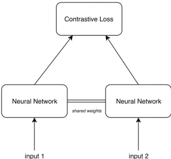
Siamese Networks

Siamese networks are networks which follow a specific kind of architecture. They consist of two identical networks with shared weights which are used to embed usually two inputs. The embeddings of these inputs and then compared in the objective function using a contrastive loss. The goal is not to classify, but rather to differentiate between inputs. For example, in Chapter 6 we look into training siamese-like networks for answer

(46)

3.6. Summary 3. A Deep Learning Primer

selection where we train the model to differentiate between correct context-candidate pairs and wrong (distractor) context-candidae pairs.

3.6

Summary

The above brief introduction to some of the most important deep learning and NLP concepts used throughout this thesis will help us as we present new models in subse-quent chapters. Throughout, I will refer the reader back to this chapter whenever we use, with little description, any of the techniques described above. Already in the next chapter, we will make heavy use of almost all that has been introduced here.

(47)

Part II

(48)

Chapter 4

A Detailed Ablation Study of the

BiDAF Model

This chapter contains our first contribution.

4.1

Introduction

Since the release of the Stanford Question Answering Dataset (SQuAD) [105] in 2016, dozens of models have competed on it. Although all different, they are comprised of many of the same or similar components. Just as LSTMs have become a staple compo-nent of many NLP models, so too has thebi-directional attention flow (BiDAF) [123] model become a popular model within reading comprehension research. Subsequent publications have all either analyzed it, based their proposed models on it, or compared themselves against it. A review of these can be found in Section 4.7. Like other ques-tion answering models, BiDAF divides into three secques-tions. The input layers, the body layers, and the output (or answer) layers. A general description of these can found in Section 2.2.2. We describe how exactly BiDAF implements these layers in Section 4.2. In this chapter we are interest in exploring which sections of neural QA models matter most to their performance. We take BiDAF as a canonical example of a neural QA model and SQuAD as a canonical dataset and (1) explore BiDAF’s performance by conducting a detailed ablation study of its components. In so doing we attempt to isolate parts of it which contribute most to end performance; (2) We propose an extension of the BiDAF model to multiple spans.

We begin by describing the model in detail, followed by describing our modifications and ablations of it. Our changes touch on four sections of the model: (1) we analyze different attention mechanisms in the body layer used to fuse information about the

(49)

4.2. The BiDAF Model 4. A Detailed Ablation Study of the BiDAF Model

passage and query; (2) we analyze different fusion functions used to do this; (3) we look at how important the question representation is to the success of the model in the input layer; finally (4) we look at the new multi-span setting.

4.2

The BiDAF Model

4.2.1 The Input Layers

The goal of the input layers is to vectorize the question and the passage (also referred to as the context) and represent them in such a way so as to lighten the modeling burden of downstream l