Fast Uncertainty Estimation for Deep Learning Based Optical Flow

Fast Uncertainty Estimation for Deep Learning Based Optical Flow

Serin Lee

, Vincenzo Capuano

, Alexei Harvard

, and Soon-Jo Chung

Abstract— We present a novel approach to reduce the pro-cessing time required to derive the estimation uncertainty map in deep learning-based optical flow determination methods. Without uncertainty aware reasoning, the optical flow model, especially when it is used for mission critical fields such as robotics and aerospace, can cause catastrophic failures. Although several approaches such as the ones based on Bayesian neural networks have been proposed to handle this issue, they are computationally expensive. Thus, to speed up the processing time, our approach applies a generative model, which is trained by input images and an uncertainty map derived through a Bayesian approach. By using synthetically generated images of spacecraft, we demonstrate that the trained generative model

can produce the uncertainty map 100∼700 times faster than the

conventional uncertainty estimation method used for training the generative model itself. We also show that the quality of uncertainty map derived by the generative model is close to that of the original uncertainty map. By applying the proposed approach, the deep learning model operated in real-time can avoid disastrous failures by considering the uncertainty as well as achieving better performance removing uncertain portions of the prediction result.

I. INTRODUCTION

Optical flow estimation is useful for many visual per-ception applications such as robot navigation, autonomous spacecraft navigation and object detection/tracking. For ex-ample, the optical flow computed via images of an orbiting target acquired by a spacecraft chaser can be used to esti-mate the relative translational and rotational velocity of the target [1]. Since deep learning approaches have been used for the optical flow estimation, the deep learning-based methods now outperform the traditional estimators [2], [3].

Similar to other deep learning-based methods, it is often difficult to fully interpret how the trained model produces the estimate. Since it is not straightforward to decipher how deep learning models produce decision outputs, they are not yet reliable approaches for high-risk applications such as in a space mission. In particular, if the model does not know what it does not know (i.e., unknown unknowns), false predictions can be obtained with high confidence and can eventually cause catastrophic failures.

To tackle this issue there have recently been considerable efforts in explainable AI, which can be roughly divided into explaining the processing of the data, explaining the representation of the data, and creating explanation pro-ducing systems [4]. However, most recent explanable AI methods focus on explaining the processing of the data, and in particular, creating a saliency (heat) map showing an important portion of input data for making a decision [5]–[8]. Since such interpretable techniques generate the saliency map representing the importance of each pixel for the final

Bayesian Optical Flow Estimation (e.g. FlowNet2 with MC-dropout)

optical flow uncertainty map Generative Model (e.g. pix2pix) uncertainty map non-Bayesian Optical Flow Estimation

(e.g. FlowNet2) optical flow two consecutive image frames Generative Model (e.g. pix2pix) uncertainty map Training Prediction 1st training  2nd training two consecutive image frames Proposed Method Proposed Method

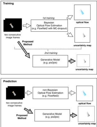
Fig. 1. Features of the proposed architecture: After the Bayesian

op-tical flow estimator is trained, the input images and their corresponding uncertainty map produced by the Bayesian estimator are used to train the generative model. The generative model learns how to map the input to the corresponding uncertainty. As a result, while the non-Bayesian optical flow estimator predicts the optical flow, the generative model can predict its corresponding uncertainty map, which is 100∼700 times faster than by the conventional Bayesian model.

decision, it would not be appropriate in the case where the decision cannot be simply represented. For example, in the case of a classification problem, we can derive the saliency map showing how much each pixel contributes to the classification result because the result can be simply represented in a probability for each class. On the other hand, in the case of the encoder-decoder network where the input image is converted into another form of image that resembles the input image (e.g., segmentation label [9], dense optical flow field), it would be harder to represent how much a part of an input contributes to a given part of the predictions.

For this reason, the Bayesian deep learning frame-work [10]–[13], which is widely used to capture uncertainty of each prediction by placing a probability distribution over the network weight, could be applied to optical flow estima-tion [14] and segmentaestima-tion [9]. However, this framework for uncertainty estimation is computationally expensive which

makes it unsuitable for real-time tasks.

As shown in Fig. 1, we overcome this challenge by employing a generative model for image-to-image trans-lation [15]. In particular, given a pair of images and its uncertainty map derived by any conventional uncertainty estimation method such as Monte Carlo (MC)-dropout [10] and deep ensemble [13], the generative model for the image-to-image translation can learn the mapping between them. The main contributions of this paper are summarized as follows:

• We show that the model uncertainty depends on its input data. Based on this, we build the generative model inferring the uncertainty with the input image.

• We establish that given input images, the generative

model can predict the uncertainty map, which is close to the original uncertainty map used for training the generative model.

• We validate that the generative model can derive the un-certainty map 100∼700 times faster than the Bayesian network, which provides training data for the generative model. It can allow the uncertainty map to be used in a real environment.

The rest of this paper is organized as follows. Related work is presented in Sec. II. In Sec. III, we modify FlowNet2 to be used in a Bayesian framework so that we can validate our approach to reduce the processing time to derive the uncertainty map. Our approach to derive the uncertainty map in real-time is presented in Sec. IV. Experimental validation using synthetic spacecraft images is presented in Sec. V.

II. RELATED WORK

Optical flow represents the pattern of apparent motion of objects, in a visual scene caused by the relative motion between an observer and those objects. Various approaches have been proposed for the estimation of optical flow. Sparse optical flow provides the flow vectors of some image features derived by feature extraction techniques, while dense optical flow gives the vectors of all pixels [16]–[18].

Machine learning approaches have been applied to optical flow estimation [2], [19]–[24]. The authors in [19] modeled local intensity pattern and local optical flow with Gaussian Mixture Models (GMM). The algorithm [20] was proposed to estimate optical flow in difficult imaging conditions by us-ing inertial estimates of the flow and combinus-ing them with a classifier. EpicFlow [21] used a sparse-to-dense interpolation relying on edge-aware geodesic distance to compute a sharp dense correspondence field. In [22], Full Flow employed a global optimization to optical flow estimation by treating classical optical flow objective function as a Markov Random Field (MRF). The epipolar constraint with a Convolutional Neural Network (CNN) was considered to perform flow matching for traffic participants in the context of autonomous driving [23]. While most of these techniques worked well in a controlled environment, they showed limited performance for practical applications in terms of scale-up and accuracy. Since FlowNet2, based on FlowNet [24], was proposed in [2], such CNN-based optical flow estimation techniques

like PWC-Net [3] have started outperforming traditional opti-cal flow estimation approaches. Although impressive perfor-mance on many popular benchmarks have been achieved, the deep learning-based optical flow estimators cannot explain about their prediction results in a way that we understand.

If there is no capability of uncertainty aware reason-ing [25] for mission critical tasks, erroneous predictions can cause disastrous consequences. In such context, in order to evaluate failure prediction scores by a deep spatio-temporal CNN and Support Vector Machine (SVM), an introspective perception framework was proposed to allow a drone to learn what is not known to it [26]. In particular, in the Bayesian deep learning framework that has been proposed to handle the uncertainty in deep neural networks, two types of uncertainties are considered in more detail – the epistemic uncertainty accounts for uncertainty included in the trained model, and the aleatoric uncertainty captures inherent observation noise [11], [12].

While the aleatoric uncertainty can be directly estimated by adding a separate branch to deep neural networks [12] that estimates the parameters of a probability distribution for this uncertainty, the epistemic uncertainty cannot be directly captured in such a way because the uncertainty of the model parameters is not considered. However, if such uncertainty is discarded, for a given input substantially different to the one used to train the model, the deep neural network can even output highly confident incorrect prediction.

Although some methods based on Markov Chain Monte Carlo (MCMC) such as Hamiltonian Monte Carlo (HMC) [27] and Stochastic Gradient Langevin Dynamics (SGLD) [28] have been proposed to derive the uncertainty, such approaches struggle with large-scale problems using high-dimensional deep neural networks. Recently, two ap-proaches have been widely used to estimate such uncertainty. MC-dropout was proposed to derive uncertainty by applying dropout at test time to randomly sample the weights of network [10]. Also, an ensemble technique using multiple networks that are randomly initialized is presented [13].

In contrast with the existing methods of estimating the uncertainty as exactly as possible [10], [13], [14], [27], [28], the objective of our methods presented in this paper is to derive the uncertainty map in real-time. It allows the uncertainty information to be used for tasks performed in a real environment. For example, the proposed real-time uncertainty estimation can be helpful for spacecraft to detect out-of-distribution input data having much higher uncertainty than the training dataset, so that the spacecraft can make an acceptable decision in real-time with non-machine learning-based methods, rather than reaching clearly unreasonable results derived by the imperfect training model.

III. OPTICAL FLOWWITHBAYESIAN DEEP LEARNING

To validate our approach designed to reduce the processing time required to derive the uncertainty included in optical flow we employed FlowNet2, which is an end-to-end learn-ing approach for optical flow estimation [2], [24], and modify

the network to adopt a Bayesian approach.

Given a dataset consisting of two consecutive image frames separated in time and their corresponding true dense optical flow, the model of FlowNet can be trained to pre-dict the dense optical flow. The FlowNetS and FlowNetC are encoder-decoder networks [29]. The encoder of the network takes an input and generates its down-sampled high-dimensional feature vectors. On the other hand, the decoder uses the feature vectors and performs up-sampling to compensate for the down-sampling. In these networks, the encoder is a normal CNN with 6 convolutional layers, and the decoder consists of translational convolutions and concatenations to get more refined results.

If the simple encoder-decoder architecture of FlowNetS is large enough, it would be enough to learn the mapping between the consecutive input frames and ground truth optical flow. However instead of using a large network and proposing optimization techniques for it, the authors [24] proposed more specialized architecture, FlowNetC which is to create two separate processing streams for each input frame. In FlowNetC after the two image features are sep-arately produced they are combined by finding correspon-dences of two feature maps using a correlation layer. In the paper [24] the authors showed that FlowNetC overfits more than FlowNetS, but it usually depends on the training dataset. Although FlowNetS and FlowNetC showed that optical flow could be derived in the framework of deep learning, the performance of other traditional methods was still better than that of FlowNet. Thus FlowNet2 [2] was proposed by stacking FlowNetC, FlowNetS, and their minor variants, as shown in Fig. 2. In the same vein, two network architectures were newly proposed for FlowNet2. FlowNetSD represents a small kernel version of FlowNetS to catch small displace-ment between two images while FusionNet was used to combine all of the results from other networks.

As we mentioned in the previous section, we apply a Bayesian deep learning framework, which is to capture the uncertainty of each prediction by placing a probability distribution over the network weights w to the FlowNet2 model. The prediction for a new input image x∗ can be written as follows

p(y∗|x∗, X, Y) =

Z

p(y∗|x∗, w)p(w|X, Y)dw (1) whereX denotes training inputs (images), Y denotes their corresponding outputs (optical flow), y∗ is the predicted optical flow, and p(w|X, Y) is the probability distribution of the network weights.

In general, computing the posterior distributionp(w|X, Y)

is intractable, so a variational distribution q(w) is used to approximate it by minimizing the Kullback-Leibler (KL) divergence.

KL(q(w)||p(w|X, Y)) (2)

For every Ki ×Ki dimensional convolutional layer i,

the above variational distribution q(wi) whose variational

parameters are Mi is used to approximate the posterior

FlowNetS Dropout Layers Encoder Network Decoder Network FlowNetC Dropout Layers Correlation & Encoder Network Decoder Network Encoder Network Encoder Network FusionNet with Dropout Layers FlowNet2 FlowNetC FlowNetS FlowNetS

FlowNetSD

Smaller kernel version of FlowNetS 

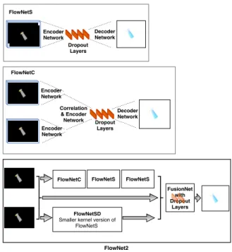
Fig. 2. Bayesian FlowNetS, FlowNetC, and FlowNet2 architectures.

FlowNet2 is a stacked architecture of FlowNetS, FlowNetC, and their minor variants. In this paper, to derive the uncertainty by the MC-dropout method, several dropout layers represented in red boxes are inserted to each component of the FlowNet2.

distribution:

zi,j ∼Bernoulli(pi)

wi=Mi·diag([zi,j]Kj=1i )

(3) where zi,j denotes Bernoulli distributed random variables

with the dropout probability pi. The dropout probability pi

can be optimized [10], but is fixed to 0.5 in this paper. In [10], [11], the authors showed that the model with the above definition approximates a Gaussian process (GP), and that minimizing the loss function of its objective function is equivalent to minimizing the KL divergence (2).

We train this model and collect the results by running the prediction at multiple times. And then, we take the meanµu,v

of the samples for the optical flow results, and the variance σ2

u,v for its model uncertainty.

µu,v= 1 M M X i=1 µu,v,i σ_u,v2 = 1 M M X i=1 (µu,v,i−µu,v)2 (4)

whereµu,v,idenotes thei-th prediction result at(u, v)ofM

tests.

To implement this Bayesian scheme called MC-dropout [10], we may need to locate the MC-dropouts after every convolutional layer. However, it is known that such approaches provide too strong regularization, so that the model learns very slowly [9]. Therefore, similar to the study in [9], we insert each of three dropout layers before and after the center of the encoder and decoder of all component networks of FlowNet2 – FlowNetS, FlowNetC, FlowNetSD,

and FusionNet, like shown as red rectangles between layers in Fig. 2.

IV. ACCELERATIONOFUNCERTAINTY ESTIMATION

As mentioned in the previous section, MC-dropout uses the dropout at test time for the random sampling [10]. Ensembling in [13] employs multiple networks with random weight initialization. These two approaches are commonly used to estimate the uncertainty of deep neural networks, but since they are based on sampling, they have the drawback of an increased inference time. MHP (Multiple Hypotheses Predictions)-WTA (Winner-Takes-All) loss in [14] could avoid the multiple forward passes of the sampling-based un-certainty estimation, but increasing the number of hypotheses can result in rapid performance degradation.

Since the uncertainty estimation methods are characterized by high computational cost, they are not suitable for mission critical tasks that require reliable uncertainty information in real-time. Under the assumption that the uncertainty depends on the input, as we will see in Sec. V-B, we propose to employ the generative model for image-to-image translation called pix2pix [15], which is to translate one possible rep-resentation of an image into another (e.g., black and white photo to color, map to satellite image, sketch to object, and segmented image to photo). As we described in Fig. 1, given a pair of input images and its corresponding uncertainty map derived by any method such as MC-dropout, ensembling, and MHP, the pix2pix based on conditional generative adversarial networks (cGANs) can learn the mapping between them, thus directly derive the uncertainty map faster than other uncertainty estimation methods by a forward pass through the network, given a new input image.

The GANs architecture is composed of two deep neural networks [30]: the generator network creates a plausible candidate image from random noise vector while the dis-criminator network evaluates it. That is, the generator net-work tries to “fool” the discriminator netnet-work by producing more realistic images, but the discriminator network aims to distinguish well whether its input image is real or generated (fake). The cGANs are a conditioned version of the GANs – its generator and discriminator networks receive some additional conditioning input image. Based on the input image, cGAN learns the mapping from the input image to another representation of the input image, as shown in Fig. 3. We use a smaller version of U-net [33] for the generator netG, and a conventional CNN for the PixelGAN discrimi-nator networkD[15] with the following objective functions.

LcGan(G, D) =Ex,y[logD(x, y)]

+_Ex,z[log(1−D(x, G(x, z)))]

(5) where cGANs learn a mapping from input images x and random noise vectorz to uncertainty map y,G:{x, z} →

y. Note thatDis trained to detect the fake image fromGas well as possible. Unlike a traditional GAN, cGAN does not takezfrom the latent space as input. Instead, the randomness in cGAN stems from the use of dropout layers. In addition,

Generator Network (Small U-net) Discriminator Network ground truth uncertainty map generated uncertainty map training DB

predicted uncertainty map ground tuth or generated? y G(x, z) prediction path two sequential images

Fig. 3. cGANs architecture for uncertainty estimation. The solid arrow

represents the training flow, and dotted arrow the prediction. Once the model is trained, the uncertainty map can be directly derived from the input images by a forward pass represented in the dotted arrow through the trained U-net.

Fig. 4. Example of the synthetic images, generated with open source 3D

creation suite Blender [31], from the 3D model of the Aura spacecraft [32]. To validate our architecture proposed to accelerate the uncertainty estima-tion, these images are used to train the FlowNet2 with MC-dropout model.

sinceGshould be able to create the output near the ground truth uncertainty map,L1distance is added to the objective function.

L1(G) =Ex,y,z[||y−G(x, z)||1] (6) Thus, the final objective function is

arg minG maxDLcGan(G, D) +λL1(G) (7) whereλis the weight of theL1loss (6).

L2 loss may be used in the above objective function, but it is well known that it can cause blurry results [15]. Also, since the transposed convolution layers of the U-net can produce checker board artifacts on the reconstructed image, using upsampling before convolutional layers instead of the transposed convolution may be helpful to avoid such noise [34].

V. EXPERIMENTAL RESULTS

A. Synthetic Data Preparation

Our proposed approach can be generally employed for other datasets. However, to validate our proposed architec-ture depicted in Figs. 1–3, we generated 26,400 sequential pairs of realistic synthetic images of the Aura spacecraft model [32] with various poses and different lighting con-ditions by using the open-source 3D suite Blender [31]. Figure 4 shows three representative generated images. We

then divided the dataset into two groups: 80% of the data are used as a training set, and the remaining 20% as a test set.

B. Uncertainty Estimation and Interpretation

We trained our FlowNet2 with MC-dropout model using our synthetic dataset and stochastic gradient descent (SGD) with the learning rate of 1e-5. The uncertainty map generated by the FlowNet2 with MC-dropout model was used to verify our proposed approach to reduce the processing time to derive the uncertainty map.

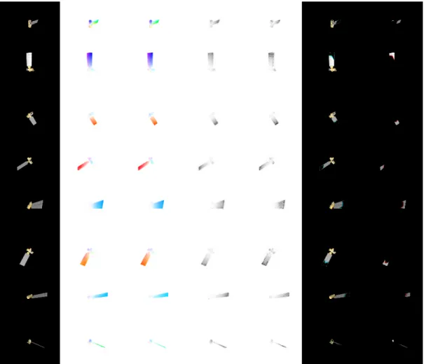
Figure 7 shows some prediction results with the uncer-tainty map for the test dataset. The optical flow is represented in the Middlebury color coding [35], in which the color represents the direction of optical flow, and the smaller vectors are represented in lighter color. With a careful comparison between the original image and uncertainty map in the figure, we can find that our trained model mostly has high confidence in the interior parts of the images, but low confidence around the image edge. This finding is confirmed in other literature studies which show that capturing sharp discontinuous optical flow occurred on motion boundary, which is a subset of image edges, is challenging [21], [36]– [38].

C. Evaluation of Accelerated Uncertainty Estimation

Our proposed method is based on the pix2pix generative model to directly derive the uncertainty map from the input images. To train the generative model we used the images for training and testing FlowNet2 with MC-dropout model, and the uncertainty maps obtained from 48 samples by the trained FlowNet2 with MC-dropout model. The training was performed with the Adam optimizer, the learning rate of 2e-4, andλ= 1000. The results are also shown in Fig. 7. The comparison of the inference times to derive the uncertainty map is represented in Table I.

TABLE I

INFERENCE TIME COMPARISON

Case Time [s]

8 samples [10] 0.16

48 samples [10] 0.99

pix2pix trained by 48

samples from MC-dropout 0.0013

To evaluate how much the uncertainty derived by the generative model for the pix2pix is accurate, we use a sparsification plot, which is widely used for this purpose [14]. If some parts of the input data with the uncertainty are grad-ually removed, the error should be monotonically dropped. Figure 5 shows that the average endpoint error (AEPE) is decreased as each fraction of pixels with the highest uncertainty is removed. The AEPE was derived by

AEP E= 1 N X i q (ui−uGTi )2+ (vi−viGT)2 (8) 0.0 0.2 0.4 0.6 0.8 1.0

Fraction of Removed Pixels

0.0 0.2 0.4 0.6 0.8 1.0

Normalized Average End Point Error

MC Dropout Estimation by Pix2Pix Oracle

Fig. 5. Sparsification plot of MC-dropout and pix2pix methods. The trained FlowNet2 with MC-dropout model creates the uncertainty map, which will be used for training the pix2pix generative model, as shown in Fig. 1. Figure 3 shows that the pix2pix generative model predicts the uncertainty map through the feed-forward network. In this plot, the ”oracle” represents true error, which is usually considered as ground truth uncertainty.

Fig. 6. Uncertainty map of out-of-distribution data derived by the proposed uncertainty estimation

where(uGT_i , v_iGT)denotes the ground truth optical flow for the predicted optical flow(ui, vi). It means the average of all

the distances inN pixels between the predicted and ground truth optical flow.

The plot also shows that the uncertainty estimation derived by the pix2pix generative model is quite similar to that of the FlowNet2 with MC-dropout model used for training the generative model.

Figure 6 also shows that the proposed uncertainty estima-tion can be used to reliably detect out-of-distribuestima-tion data. The images from CIFAR-10 dataset, which are quite different from our training dataset, and their randomly translated images were used for the inputs to the trained cGAN model. Comparing with the Fig. 7, its uncertainty is clearly out of the desired range of uncertainty acquired from the training dataset.

VI. CONCLUSION

Deep learning-based optical flow estimators, which have outperformed traditional optical flow methods, are useful

Fig. 7. Sample results of the FlowNet2 with MC-dropout and the uncertainty map by the pix2pix generative model - From left: first input image, predicted optical flow, ground truth optical flow, uncertainty by the pix2pix generative model, uncertainty obtained from 48 sample predictions by the FlowNet2 with MC-dropout, image parts with low and high uncertainty derived by the proposed generative model-based uncertainty estimation. The darker color in the uncertainty map represents more uncertain prediction.

for many applications such as pose estimation and object detection/tracking of drones, mobile robots, and spacecraft. However, if the uncertainty included in the optical flow estimation is not taken into consideration, it can lead to very unreliable and inaccurate estimation results. Although conventional uncertainty estimation methods output useful uncertainty maps to handle this issue, they are computa-tionally expensive. Thus, we presented a novel approach to significantly improve the processing time required to derive the uncertainty map by adapting the generative model that was trained by the input data and uncertainty map derived by applying the MC-dropout to a modified FlowNet2 network. The experimental results showed that our approach was able to obtain the uncertainty map 100∼700 times faster than the original FlowNet2 with MC-dropout, and that the obtained uncertainty map was close to the original uncertainty map. The proposed approach will help the trained model to avoid disastrous failures and increase the performance in real-time. Future work includes applying our approach to the pose estimation of spacecraft and generalizing this approach to other areas such as segmentation and regression.

ACKNOWLEDGMENT

The authors thank A. Rahmani, A. Santamaria-Navarro, and F. Y. Hadaegh for their technical guidance.

REFERENCES

[1] V. Capuano, K. Kim, A. Harvard, and S.-J. Chung, “Monocular-based pose determination of uncooperative space objects,”Acta Astronautica, vol. 166, pp. 493–506, 2019.

[2] E. Ilg, N. Mayer, T. Saikia, M. Keuper, A. Dosovitskiy, and T. Brox, “Flownet 2.0: Evolution of optical flow estimation with deep net-works,” inProc. IEEE Conf. Computer Vision and Pattern Recognition (CVPR), Honolulu, HI, 2017, pp. 1647–1655.

[3] D. Sun, X. Yang, M.-Y. Liu, and J. Kautz, “PWC-Net: CNNs for optical flow using pyramid, warping, and cost volume,” inProc. IEEE Conf. Computer Vision and Pattern Recognition (CVPR), Salt Lake City, UT, 2018, pp. 8934–8943.

[4] L. H. Gilpin, D. Bau, B. Z. Yuan, A. Bajwa, M. Specter, and L. Kagal, “Explaining explanations: An overview of interpretability of machine

learning,” inProc. 5th IEEE Int. Conf. Data Science and Advanced

Analytics (DSAA), Turin, Italy, 2018, pp. 80–89.

[5] M. T. Ribeiro, S. Singh, and C. Guestrin, “”why should i trust you?”:

Explaining the predictions of any classifier,” in Proc. 22nd ACM

SIGKDD Int. Conf. Knowledge Discovery and Data Mining, San Francisco, CA, 2016, pp. 1135–1144.

[6] R. R. Selvaraju, M. Cogswell, A. Das, R. Vedantam, D. Parikh, and D. Batra, “Grad-cam: Visual explanations from deep networks via gradientbased localization,” inProc. IEEE Int. Conf. Computer Vision (ICCV), Venice, Italy, 2017, pp. 618–626.

[7] S. A, G. P, and K. A, “Learning important features through propagating

activation differences,” in Proc. 34th Int. Conf. Machine Learning

(ICML), Sydney, Australia, 2017, pp. 3145–3153.

[8] S. Bach, A. Binder, G. Montavon, F. Klauschen, K.-R. M¨uller, and W. Samek, “On pixel-wise explanations for non-linear classifier decisions by layer-wise relevance propagation,”PLOS ONE, vol. 10, 2015.

[9] A. Kendall, V. Badrinarayanan, and R. Cipolla, “Bayesian segnet: Model uncertainty in deep convolutional encoder-decoder architectures

for scene understanding,” in Proc. British Machine Vision Conf.

(BMVC), London, United Kingdom, 2017, pp. 57.1–57.12.

[10] Y. Gal and Z. Ghahramani, “Dropout as a bayesian approximation: representing model uncertainty in deep learning,” inProc. 33rd Int. Conf. Machine Learning (ICML), New York City, NY, 2016, p. 1050–1059.

[11] Y. Gal, “Uncertainty in deep learning,” Ph.D. dissertation, Dept. Eng., Univ. of Cambridge, Cambridge, United Kingdom, 2016.

[12] A. Kendall and Y. Gal, “What uncertainties do we need in bayesian deep learning for computer vision?” in Proc. 31st Int. Conf. Neural Information Processing Systems (NIPS), Long Beach, CA, 2017, pp. 5580–5590.

[13] B. Lakshminarayanan, A. Pritzel, and C. Blundell, “Simple and scalable predictive uncertainty estimation using deep ensembles,” in

Proc. 31st Int. Conf. Neural Information Processing Systems (NIPS), Long Beach, CA, 2017, pp. 6405–6416.

[14] E. Ilg, ¨O. C¸ ic¸ek, S. Galesso, A. Klein, O. Makansi, F. Hutter, and T. Brox, “Uncertainty estimates and multi-hypotheses networks for

optical flow,” in Proc. European Conf. Computer Vision (ECCV),

Munich, Germany, 2018, pp. 677–693.

[15] P. Isola, J.-Y. Zhu, T. Zhou, and A. A. Efros, “Image-to-image translation with conditional adversarial networks,” inProc. IEEE Conf. Computer Vision and Pattern Recognition (CVPR), Honolulu, HI, 2017, pp. 5967–5976.

[16] B. K. P. Horn and B. G. Schunck, “Determining optical flow,”Artificial Intelligence, vol. 17, pp. 185, 203, 1981.

[17] B. D. Lucas and T. Kanade, “An iterative image registration technique

with an application to stereo vision,” in Proc. 7th Int. Jt. Conf.

Artificial intelligence (IJCAI), Vancouver, BC, Canada, 1981, pp. 674– 679.

[18] G. Farneb¨ack, “Two-frame motion estimation based on polynomial expansion,” inProc. 13th Scandinavian Conf. Image Analysis (SCIA), Halmstad, Sweden, 2003, pp. 363–370.

[19] D. Rosenbaum, D. Zoran, and Y. Weiss, “Learning the local statistics of optical flow,” inProc. 26th Int. Conf. Neural Information Processing Systems (NIPS), Lake Tahoe, NV, 2013, pp. 2373–2381.

[20] R. Kennedy and C. Taylor, “Optical flow with geometric occlusion estimation and fusion of multiple frames,” inProc. Int. Work. Energy Minimization Methods in Computer Vision and Pattern Recognition (EMMCVPR), Hong Kong, China, 2015, pp. 364–377.

[21] J. Revaud, P. Weinzaepfel, Z. Harchaoui, and C. Schmid, “Epicflow: Edge-preserving interpolation of correspondences for optical flow,” in

Proc. IEEE Conf. Computer Vision and Pattern Recognition (CVPR), Boston, MA, 2015, pp. 1164–1172.

[22] Q. Chen and V. Koltun, “Full flow: Optical flow estimation by global optimization over regular grids,” inProc. IEEE Conf. Computer Vision and Pattern Recognition (CVPR), Las Vegas, NV, 2016, pp. 4706– 4714.

[23] M. Bai, W. Luo, K. Kundu, and R. Urtasun, “Exploiting semantic

information and deep matching for optical flow,” inProc. European

Conf. Computer Vision (ECCV), Amsterdam, The Netherlands, 2016, pp. 154–170.

[24] A. Dosovitskiy, P. Fischer, E. Ilg, P. Hausser, C. Hazirbas, V. Golkov, P. van der Smagt, D. Cremers, and T. Brox, “Flownet: Learning optical flow with convolutional networks,” inProc. IEEE Int. Conf. Computer Vision (ICCV), Santiago, Chile, 2015, pp. 2758–2766.

[25] Gustafsson, F. K, Danelljan, Martin, Sch¨on, and T. B, “Evaluating scalable bayesian deep learning methods for robust computer vision,” in Proc. IEEE/CVF Conf. Computer Vision and Pattern Recognition Workshop (CVPRW), 2020, pp. 1289–1298.

[26] S. Daftry, S. Zeng, J. Bagnell, and M. Hebert, “Introspective percep-tion: Learning to predict failures in vision systems,” inProf. IEEE/RSJ Int. Conf. Intelligent Robots and Systems (IROS), Daejeon, Korea, 2016, pp. 1743–1750.

[27] R. M. Neal, “Bayesian learning for neural networks,” Ph.D. disserta-tion, Dept. Comp. Sci., Univ. of Toronto, Toronto, Canada, 1995.

[28] M. Welling and Y. W. Teh, “Bayesian learning via stochastic

gradi-ent langevin dynamics,” inProc. 28th Int. Conf. Machine Learning

(ICML), Bellevue, WA, 2011, pp. 681–688.

[29] V. Badrinarayanan, A. Kendall, and R. Cipolla, “Segnet: A deep convolutional encoder-decoder architecture for image segmentation,”

IEEE Trans. Pattern Analysis and Machine Intelligence (TPAMI), vol. 39, no. 12, pp. 2481–2495, 2012.

[30] I. Goodfellow, J. Pouget-Abadie, M. Mirza, B. Xu, D. Warde-Farley, S. Ozair, A. Courville, and Y. Bengio, “Generative adversarial nets,” in

Proc. 27th Int. Conf. Neural Information Processing Systems (NIPS), Montr´eal, Canada, 2014, pp. 2672–2680.

[31] Blender, “Blender,” 2020, accessed on 07.30.2020. [Online]. Available: https://www.blender.org

[32] C. M. Garcia, “Nasa 3d resources,” 2020, accessed on 07.30.2020. [Online]. Available: https://nasa3d.arc.nasa. gov/detail/aura-eoe3d [33] O. Ronneberger, P.Fischer, and T. Brox, “U-net: Convolutional

net-works for biomedical image segmentation,” inProf. Medical Image

Computing and Computer-Assisted Intervention (MICCAI), Munich, Germany, 2015, pp. 234–241.

[34] A. Odena, V. Dumoulin, and C. Olah, “Deconvolution and checkerboard artifacts,” 2016, accessed on 07.30.2020. [Online]. Available: https://distill.pub/2016/deconv-checkerboard/

[35] S. Baker, D. Scharstein, J. Lewis, S. Roth, M. Black, and R. Szeliski,

“A database and evaluation methodology for optical flow,” inProc.

IEEE Int. Conf. Computer Vision (ICCV), Rio de Janeiro, Brazil, 2007, pp. 1–8.

[36] P. Weinzaepfel, J. Revaud, Z. Harchaoui, and C. Schmid, “Learning

to detect motion boundaries,” inProc. IEEE Conf. Computer Vision

and Pattern Recognition (CVPR), Boston, MA, 2015, pp. 2578–2586. [37] X. Yin, X. Dai, X. Wang, M. Zhang, D. Tao, and L. Davis, “Deep motion boundary detection,”arXiv preprint arXiv:1804.04785, 2018. [38] C. Peng, S. Lo, J. Huang, and A. C. Tsoi, “Human action segmentation based on a streaming uniform entropy slice method,”IEEE Access, pp. 16 958–16 971, 2018.