Supply chains with or without upstream
competition?
Chrysovalantou Milliou*
Universidad Carlos III de Madrid, Department of Economics, Getafe (Madrid) 28903, Spain
23 February 2004
Abstract
We investigate a final good producer's incentives to engage in an exclusive relation with one of two competing input suppliers in an environment where both market sides undertake quality-enhancing investments and bargain over their terms of trade. Although the investments’ compatibility is full only under exclusivity, we still find that the investments under exclusivity can be lower than that under non-exclusivity. We also find that there exist cases in which although the investments are higher under exclusivity, the final good producer chooses non-exclusivity. Finally, we find that the final good producer’s choice of exclusivity in equilibrium is never welfare detrimental.
JEL classification: L22; L42; L14; L15
Keywords: Exclusive Dealing; Supply Chains; Quality-enhancing Investments; Compatibility; Bargaining
* E-mail: [email protected]. I am grateful to Massimo Motta, Emmanuel Petrakis and Karl Schlag for their valuable comments and discussions. I would also like to thank Vincenzo Denicoló and Margaret Slade for their helpful suggestions. Full responsibility for all shortcomings is mine.
1. Introduction
Why do some final good producers develop exclusive relations with their input suppliers while others tend to shop around among a large number of suppliers? What are the private and the social costs and benefits of an exclusive supply chain structure relative to a non-exclusive one? At first glance the two distinct supply chain structures differ in their level of upstream competition. Accordingly, some would argue that a supply chain structure with an exclusive input supplier increases the upstream monopoly power, and thus, it is not only anticompetitive, but it is also undesirable from the final good producer’s point of view.
Contrary to the above reasoning and to what it would have been expected in a world in which technology has considerably decreased transaction and search costs, there is growing evidence that firms do not tend to shop around among a large number of suppliers based purely on price. What is instead observed is that large manufacturing firms in the U.S. and elsewhere tend to restrict the upstream competition by developing exclusive partnerships with their input suppliers. One of the most prominent examples of this trend is observed within the business-to-business (B2B) e-commerce. Many firms instead of obtaining their inputs from 'public' B2B e-marketplaces, in which they have the ability of trading with a large number of participating suppliers, they choose instead to create their own 'private' e-marketplaces, in which they trade with their exclusive suppliers.
One of the reasons commonly used to explain this trend is that firms are placing an increased emphasis on product quality and that they develop a better coordination of their quality-enhancing investments by dealing with a single supplier. The better coordination combined with the fact that a supplier enjoys a higher share of the supply chain’s surplus under an exclusive relation rather than under a non-exclusive one may in turn increase the level of the quality-enhancing investments.
The objective of this paper is to investigate a final good producer's incentives to adopt a supply chain structure characterized by an exclusive buyer-supplier relation. We consider the following model. A downstream monopolist - an input buyer - decides at the beginning of the game whether or not it will engage in an exclusive relation with one of two potential input suppliers. After the form of the buyer-supplier relations has been decided, both the buyer and the suppliers undertake investments that enhance the quality of their products. Finally, after the firms have undertaken their investments, but
before the buyer sells its final product in the downstream market, bargaining over the terms of a two-part tariff contract takes place between the buyer and the supplier(s).
We assume that that the compatibility of the buyer’s and the supplier’s investments is full only under exclusivity. This assumption captures the fact that under exclusivity, the relations between the buyer and its exclusive supplier are tighter, and thus, the coordination of their investments is higher than that under non-exclusivity.1 Although the compatibility of the investments is full only under exclusivity, we still find that the investments under exclusivity can be lower than that under non-exclusivity. In particular, this holds both for the buyer’s and the supplier’s investments when the buyer’s bargaining power is sufficiently low. The intuition for this result is as follows. Under non-exclusivity, the buyer does not enjoy the full compatibility of its investments but it does enjoy a compensation for its outside option. While the lack of full compatibility has a negative impact on the buyer’s incentives to invest, its compensation for the outside option has a positive impact since its investments increase the value of its outside option. Under exclusivity, the outside option is absent but the buyer enjoys the full compatibility of its investments which in turn increases its incentives to invest. When the buyer’s bargaining power is low, the effect of the outside option dominates and the buyer’s investments are higher under non-exclusivity than under exclusivity. This is so because when the buyer’s bargaining power is low, the buyer receives a higher share of its outside option under non-exclusivity, and thus, its incentives to invest under non-exclusivity become even stronger. Strategic complementarity between the buyer’s and the supplier’s investments leads to a similar behavior of the supplier’s investments.
Regarding the equilibrium supply chain structure, we find that the buyer opts for exclusivity only when its bargaining power is sufficiently high. It is not surprising that this result is due to a big extent to the behavior of the quality-enhancing investments. In particular, when the buyer opts for exclusivity, both the buyer's and the supplier's investments, as well as the total effective investments (i.e. the product's total quality level) are higher under exclusivity than under non-exclusivity. What is though surprising is that there exist cases in which the buyer chooses non-exclusivity, although the investments are higher under exclusivity. In other words, the quality-enhancing investments are not the only force at work. The buyer's decision is also affected by the
1 In an extension of the basic model, included in Section 6, we endogenize this assumption and provide conditions under which holds.
fact that there is competition among the suppliers only in the non-exclusivity case. Due to the suppliers' competition, the buyer is always compensated for its outside option. In other words, for the same level of total effective investments in the two cases, the buyer has effectively higher bargaining power during the contract terms negotiations in the case of non-exclusivity where it has the outside option to deal with an alternative supplier, than in the case of exclusivity where there is no outside option.
Regarding welfare, we find that there exist cases in which although the buyer chooses non-exclusivity, welfare is not higher under non-exclusivity. However, we also find that there exist no cases in which the buyer’s choice of exclusivity in equilibrium is welfare detrimental. Hence, from an antitrust policy’s perspective, although our results indicate that the social and the private incentives do not always coincide, they still provide an argument against the view that exclusive dealing is an anticompetitive practice, in the cases at least that the exclusivity is initiated by downstream final good producers.
There is an extensive literature that examines the incentives to undertake noncontractible investments in bilateral monopoly settings, that is, in settings with one buyer and one supplier (e.g. Williamson, 1985, Tirole, 1986, Grossman and Hart, 1986, Hart and Moore, 1988). Although bilateral monopoly is not the only situation where trade occurs, the analysis of incentives in settings in which suppliers do not have the monopoly power in the upstream market has not attracted adequate attention. The same holds for the analysis of the choice among supply chain structures characterized by either exclusive or non-exclusive relations.2
Segal and Whinston's (2000) paper is, to the best of our knowledge, the only formal theoretical attempt that examines the conditions under which buyer initiated exclusive contracts may be privately and socially valuable for protecting noncontractible
investments.3 Their main finding is that when only one of the suppliers undertakes
investments, the exclusivity has no impact on its investments level when the latter do not affect the surplus generated by the buyer and the other supplier. Our paper differs
from theirs on several grounds.4 First, in the paper of Segal and Whinston the
2 Even in cases where there is bilateral monopoly, that monopoly will be often created by a choice between alternative suppliers in a prior period.
3 For an informal discussion of the potential impact of exclusivity on investments see Klein (1988) and Klein et al. (1978).
4 The same differences apply also in the comparison of our analysis with that of De Meza and Selvaggi (2003) which focuses on the reverse market structure: an upstream input monopolist and two potential downstream input buyers.
exclusivity provision itself can be renegotiated ex post, that is, after the investments have been undertaken. In our paper, we focus instead in the case that the exclusivity provision can not be renegotiated.5 Second, while we consider a bargaining game over the terms of trade in which the buyer and the supplier(s) make take-it-or-leave-it offers with probabilities equal to their respective bargaining powers, Segal and Whinston use a cooperative solution concept for the multi-party bargaining game. Third, we consider a novel distinction between the case of exclusivity and non-exclusivity, the compatibility of the buyer's and supplier's investments in the quality enhancement of their products.
Our work is also related to the vertical restraints literature on exclusive dealing. Most of this literature has focused on supplier initiated exclusive dealing contracts. That is, it has mostly analyzed the suppliers' decision whether or not to offer exclusive dealing contracts to potential buyers of their products, taking into account the effects of such a decision on the buyers’ and/or the suppliers’ investments (see e.g. Marvel, 1982, Besanko and Perry, 1993, Bernheim and Whinston, 1998). In other words, this literature has not analyzed the case of final good producer's initiated exclusive dealing contracts. Our focus in the case in which the downstream firm is a producer of one final product and not a multi-product firm is in sharp contrast with this trend of the literature in which under non-exclusivity, the downstream firms are multi-product retailers, selling the competing final products of all the upstream firms. Undoubtedly this literature has shed some light on the antitrust issues arising in cases with supplier initiated exclusivity contracts, but has not examined the antitrust implications of buyer initiated exclusivity contracts.
The remainder of the paper is organized as follows. In Section 2, we describe our basic model. In Section 3, we analyze the non-exclusivity case. In Section 4, we analyze the exclusivity case and discuss the impact of exclusivity on the investment incentives. In Section 5, we analyze the buyer's decision regarding exclusivity and examine the welfare implications of our model. In Section 6, we extend the model by considering the case in which compatibility can be the outcome of the suppliers' strategic choice. Finally, in Section 7, we conclude and propose avenues for further research. All the proofs are included in the Appendix.
5 A simple justification for our approach (the same approach is also adopted in the vertical restraints literature on exclusive dealing) is that an exclusive dealing contract can also include a technological commitment that not only affects the compatibility of the buyer's and its exclusive supplier's investments but it also makes trade with the alternative suppliers not possible, e.g. the buyer decides to locate its plant far away from alternative suppliers and next to its exclusive supplier.
2. The Model
We consider an industry consisting of a downstream firm - input buyer, denoted by
B, and two upstream firms - potential input suppliers, each denoted by Si, with i = 1, 2.6
There is an one-to-one relation between the input and the final product produced by the buyer. Each of the two input suppliers faces a constant marginal cost of production, denoted by c.
We analyze a full information four-stage game (see Fig. 1). In the first stage, the buyer decides whether or not it will engage in an exclusive relation with one of the suppliers. The exclusive relation can be established through the use of an exclusive dealing contract that specifies a prohibitive compensation that the buyer must pay to its exclusive supplier in case it obtains the input from the non-exclusive supplier.7
In the second stage, the buyer B and its potential suppliers S1 and S2 simultaneously and independently choose their investment levels, b, s1 and s2 respectively. Each firm’s investments lead to an increase in the quality of its own product. We assume that the higher is the quality of the input used in the final product, the higher is the latter’s quality. Moreover, we assume that consumers have a higher willingness to pay for products of higher quality. In particular, the inverse demand function for the final product is:
p=a+θˆ(b+si)−q, a>c≥0 (1) where q and p are respectively the quantity and the price of the final product. The subscript i = 1, 2 indicates the supplier from which the buyer obtains the input. The parameter θˆ captures the degree of compatibility of the buyer’s and its input supplier’s
investments. Low values of θˆ reflect low compatibility of the outcomes of their
research projects (e.g. bad matching due to lack of coordination). We assume that compatibility is full only under exclusivity. In particular, θˆ=1 under exclusivity and
, ˆ θ
θ = with 0≤θ <1, under non-exclusivity. The investments of both the buyer and the
6 As it will become clear in the model’s solution, we would obtain the same results if we had assumed instead that the number of supplies is n, with n ≥2.
7 Note that the exclusive dealing contract does not include any other term besides the exclusivity provision.In particular, it specifies neither the future investments levels nor the terms of future trade. In this sense it is an 'incomplete contract'. A justification for this assumption is that the contractual arrangement for an exclusive buyer-supplier relation has longer run characteristics than their specific terms of trade, given that the latter could be easier changed. For additional justifications of this type of contracts see Grossman and Hart (1986), and Hart and Moore (1988).
suppliers are subject to diminishing returns to scale, captured by the quadratic form of their cost functions: b2 2 and 2 2
i
s , i = 1, 2.
In the third stage, bargaining over a two-part tariff contract, consisting of a wholesale price wi and a franchise fee Fi, takes place among the buyer and its potential
input suppliers. Under exclusivity the buyer bargains only with its exclusive supplier, while under non-exclusivity it bargains simultaneously with both S1 and S2. In modeling the bargaining game, we adopt the approach used by Chemla (2003) and Rey and Tirole (2003). In particular, in the exclusivity case, a take-it-or-leave-it offer over wi and Fi is
made with probability β by the exclusive supplier and with probability 1-β by the buyer. Similarly, in the non-exclusivity case, take-it-or-leave-it offers over wi and Fi, are made
simultaneously and independently by S1 and S2 with probability β and with probability 1-β by the buyer. The parameter β, 0<β<1, denotes the suppliers’ bargaining power.
In the last stage of the game, the buyer chooses the quantity of its final good and produces it using the input obtained according to the terms of trade specified in the previous stage.
We derive the subgame perfect Nash equilibria in pure strategies of the above four-stage game. Since the upstream firms are identical, there are two second-four-stage subgames to consider, the subgame with non-exclusivity and the subgame with exclusivity. In what follows, we start by analyzing the two subgames separately and then we move to the analysis of the first stage.
3. Non-Exclusivity
In this section we derive the equilibrium for the non-exclusivity case, that is, the case in which the buyer is free to obtain its input from any of the two suppliers. We proceed by backward induction.
In the fourth stage, the buyer chooses the output that maximizes its gross profits:
(
a b s q w)
q q s b wi i i i B( , , , )= +θ( + )− − π (2)The subscript i = 1, 2 simply specifies the supplier from which the buyer obtains its input.8 From the first order condition of (2) with respect to q, we obtain the equilibrium
8 We assume w.l.o.g. that the buyer always buys all its input quantity from one supplier. When the buyer is indifferent between purchasing from any one of the two suppliers, we can distinguish among two cases. First, if the suppliers offer different input qualities, the buyer will always buy from the high quality supplier – this is a reasonable tie-breaking rule. Second, if the two suppliers offer the same input quality and the same terms of trade, it makes no difference for our analysis if the buyer buys all the input quantity from one of them or if it splits this quantity between the two in any arbitrary way.
quantity of the final good: 2 ) ( ) , , ( i i i i w s b a s b w q = +θ + − (3) In the third stage of the game, where the bargaining takes place simultaneously among the buyer and its potential suppliers, we distinguish among the following two cases, for i, j = 1, 2 and i ≠ j:
(a) si = sj ≥ 0: When the suppliers offer the same input quality, competition among
them results not only in both of them making the same contract offer, but also in making
an offer that leaves them with zero profits. Formally, each Si makes an offer that
maximizes the buyer’s profits subject to the constraint that its own profits are non-negative:
(
)
i i i F w F w s b a Max i i + + − − 4 ) ( 2 , θ (4) s.t. 0 2 ) ( ) ( i − + + i − i +Fi ≥ w s b a c w θThe constraint in (4) is binding, and thus, the supplier's maximization problem is equivalent to the maximization of the buyer’s and supplier’s joint profits. As a result, both suppliers end up offering wholesale prices which are equal to the marginal cost of production, wi = w j = c, and franchise fees which are equal to zero, Fi = F j= 0.
When the buyer makes the contract offer, itchooses wi and Fiin order to maximize
its profits subject to the constraint that Si's profits are non-negative. In other words, the
buyer’s problem is equivalent to (4). As a result, the buyer offers the same contract terms with the suppliers.
It follows that the expected net profits of the two suppliers are zero in the case that they have not undertaken any investments, and negative otherwise.
(b) si > sj ≥ 0: When one of the suppliers offers a higher input quality than its
competitor, then the two suppliers face two different maximization problems. The high input quality supplier maximizes its profits subject to the constraint that the buyer will have no incentives to buy from the low input quality supplier, i.e.
i i i i F w F w s b a c w Max i i − + + − + 2 ) ( ) ( , θ (5)
(
)
(
)
j j j i i i w F a b s w F s b a t s + + − − ≥ + + − − 4 ) ( 4 ) ( . . 2 2 θ θAt the same time, the low input quality supplier maximizes the buyer’s profits subject to its own profits being non-negative. Just like in case (a), this translates into optimally setting wj = c and Fj = 0. Due to this and to the fact that the constraint in (5) is binding,
the maximization problem of the high input quality supplier reduces to:
(
) (
)
(
)
4 ) ( 4 ) ( 2 ) ( ) ( 2 2 a b s c w s b a w s b a c w Max i i i i j i wi − + + − − + + + − + + − θ θ θ (6)This is equivalent to the maximization of the buyer’s and the high input quality supplier’s incremental joint profits (i.e. those above the buyer’s 'outside option') and it is easy to see that it leads again to wi = c. However, it does not lead to a zero franchise
fee, it leads instead to:
(
)
(
)
4 ) ( 4 ) (b s c 2 a b s c 2 a F i j i − + + − − + + = θ θ (7)Note that when the supplier with the high input quality makes the contract offer, it cannot extract through the franchise fee all the buyer’s profits. Instead, it has to compensate the buyer for its 'outside option', that is, for the profits that the buyer would make in case it accepted the contract offered by the other supplier.9
When the buyer makes the contract offer, it maximizes its profits subject to the constraint that Si's profits are non-negative. In other words, the buyer’s maximization
problem is again equivalent to (4). As a result, B offers to Si a contract in which wi = c
and Fi = 0.
It follows that the expected net profits of the low input quality supplier are zero in the case that it has not undertaken any investments, and negative otherwise. Instead, the expected net profits of the high input quality supplier are:
(
)
(
)
2 4 ) ( 4 ) ( 2 2 2 i j i S s c s b a c s b a E i − + + − − − + + =β θ θ (8)From the above analysis of the two cases we can conclude that in the second stage of the game only one of the two suppliers will invest in the quality improvement of its product.
9 Bolton and Whinston (1993) show that an alternating offer bargaining game with three players is also identical to the equilibrium of an outside option bargaining game between the parties with the largest joint surplus where the party with the alternative trading partner has an outside option of trading with its less preferred partner and obtaining the entire surplus from that trade. It is well known that in the solution to the outside option bargaining game the buyer not only obtains the corresponding to its bargaining power share of the largest surplus but it is also compensated for the surplus it could get from its outside option (see Rubinstein, 1982).
Lemma 1: Under non-exclusivity, only one of the suppliers undertakes quality enhancing investments.
Based on Lemma 1 and on the derivations included in equations (3) to (8), we characterize in the following Lemma the equilibrium outcomes under non-exclusivity.
Lemma 2: Under non-exclusivity, the level of investments chosen by the buyer and the suppliers, as well as their respective expected net profits, for i, j = 1, 2 and i ≠ j, are:
0 ; 2 2 4 ) ( 2 ; 2 2 4 ) )( 2 ( 2 2 4 2 2 2 4 2 2 2 = − − + − = − − + − − = N j N i N a c s a c s b βθ θ θ β βθ βθ θ θ β θ β θ (9) 2 2 2 4 2 2 2 4 4 6 2 2 4 3 2 ) 2 2 4 ( 2 ) 4 4 8 2 8 ( ) ( βθ θ θ β θ β θ β θ θ β θ β − − + − + − − + − = a c EN B (10) 0 ; ) 2 2 4 ( ) 2 ( ) ( 2 2 2 4 2 2 2 2 2 = − − + − − = N S N Si E j c a E βθ θ θ β βθ θ β (11)
From the inspection of the equilibrium values in (9) it follows immediately that an increase in the compatibility of investments has a positive effect both on the buyer’s and the supplier’s investments. The effect though of an increase in the bargaining power on the investments is not so straightforward and it is included in the following Proposition.
Proposition 1: Under non-exclusivity, there exists βc(θ), increasing in θ, such that an increase in β has a positive impact both on sN and bN if β <βc(θ). While if β ≥βc(θ)
it has a positive impact only on sN.
In accordance with our expectations, an increase in the supplier’s bargaining power leads to an increase in the supplier’s investments. Contrary to this and to our expectations, the same does not hold for the buyer’s investments. In particular, an increase in the buyer’s bargaining power leads to a decrease in the buyer’s investments, provided that the buyer’s bargaining power is sufficiently high. The intuition behind this surprising result is as follows. Under non-exclusivity, the buyer gets compensated for its outside option. While the value of its outside option is increasing in the buyer’s investment, the buyer’s share of the outside option is decreasing in the buyer’s bargaining power. Given these, a decrease in the buyer’ bargaining power has two opposite effects on the buyer's investment incentives. On the one hand, it decreases the buyer's incentives because the buyer will appropriate a smaller share of its own profits in the bargaining game. On the other hand, it increases the buyer's incentives because by
undertaking higher levels of investments, it will increase its compensation for its outside option. Provided that the bargaining power of the buyer is sufficiently high, the 'outside option effect' dominates the first effect, and thus, a decrease in the buyer’s bargaining power has a positive impact on the buyer's investments.
4. Exclusivity
We turn now to the analysis of the exclusivity case, assuming without any loss of generality that the buyer awards exclusivity to supplier S1.
The last stage of the game is the same as under non-exclusivity with only one difference, the compatibility of investments is now assumed to be full. Formally, in the fourth stage the buyer chooses its output in order to maximize its gross profits:
q w q s b a q s b w B( 1, , 1, )=( + + 1− − 1) π (12)
From the first order condition of (12) with respect to q, we obtain the equilibrium
quantity of the final good:
2 ) , , ( 1 1 1 1 w s b a s b w q = + + − (13)
In the third stage, the bargaining game takes place only among buyer B and its
exclusive supplier S1. Given that S1's offer is the only offer received by B, S1 solves the following maximization problem:
1 1 1 1 , 2 ) ( 1 1 F w s b a c w Maxw F − + + − + (14) 0 4 ) ( . . 1 2 1 1− − ≥ + +b s w F a t s
The constraint is binding, and thus the maximization problem of supplier S1 turns out to be equivalent to the maximization of the buyer’s and supplier’s joint profits:
4 ) ( 2 ) ( 1 1 1 1 2 1 1 w s b a w s b a c w Maxw − + + − + + + − (15)
From the first order condition of (15) with respect to w1, it follows that w1 = c, and thus that the franchise fee is:
4 ) ( 2 1 1 c s b a F = + + − (16) Note that the franchise fee is equal to the buyer’s gross profits. In other words, when the exclusive supplier makes the contract offer, it extracts through the franchise fee all the buyer’s profits since the latter has no outside option.
In the case that B makes the contract offer to S1, B chooses w1 and F1 in order to maximize its profits subject to the constraint that S1's profits are non-negative:
1 2 1 1 , 4 ) ( 1 1 F w s b a Maxw F + + − − (17) s.t. 0 2 ) ( ) ( 1 1 1 1 + ≥ − + + −c a b s w F w
Since the constraint is binding, the buyer’s problem reduces to (15). Hence, B also
offers a wholesale price which is equal to the marginal cost, w1= c. Setting w1= c in the constraint in (17), it follows that the franchise fee offered by B is equal to zero, F1= 0.
In the second stage, S1 and B choose s1 and b respectively in order to maximize their expected net profits:10
2 4 ) ( ) , ( 2 1 2 1 1 1 s c s b a s b ES =β + + − − ; 2 4 ) ( ) 1 ( ) , ( 1 2 2 1 b c s b a s b EB = −β + + − − (18)
The equilibrium values under exclusivity derived from equations (13) to (18) are included in the following Lemma.
Lemma 3: Under exclusivity, the level of investments chosen by the buyer and its exclusive supplier, as well as their respective expected net profits are:
) )( 1 ( ); ( 1 a c b a c sE =β − E = −β − (19) 2 1 ) )( 1 ( −β − 2 +β = a c EE B ; 2 2 ) ( 2 1 β β − − = a c EE S (20)
An inspection of the equilibrium values under exclusivity reveals that contrary to the non-exclusivity case, both the buyer’s and the exclusive supplier’s investments and profits increase in their own bargaining power.
Having in hand the equilibrium investment levels for both cases, we can now compare them, and thus, we can discuss the effect of exclusivity on both the buyer's and the supplier's investments. Our main findings are summarized in the following Proposition.
Proposition 2: There exist βb(θ), βs(θ) and βe(θ), all decreasing in θ and with
, 0 ) ( = →1βb θ θ lim ( ) 0 1 = → β θ θ s lim and ( )=0 →1βe θ θ
lim such that, (i) bE >bN if and only if β β (θ)
b
<
10 Note that it follows immediately from our analysis that the non-exclusive supplier will not undertake any investments.
(ii) N i
E s
s1 > for all β when 0≤θ ≤0.839and if and only if β <βs(θ)when0.839<θ <1 (iii) 1 ( N)
i N E
E s b s
b + >θ + for all β when0≤θ ≤0.766and if and only if β <βe(θ)
when 0.766<θ <1.
According to the first part of Proposition 2, exclusivity has a negative impact on the buyer’s investment incentives only when its bargaining power is sufficiently low (Fig. 2 demonstrates the result). The intuition for this result is the following. Under non-exclusivity, the buyer does not enjoy the full compatibility of its investments but it does enjoy a compensation for its outside option. While the lack of full compatibility has a negative impact on the buyer’s incentives to invest, its compensation for the outside option has a positive impact since its investments increase the value of its outside option. Under exclusivity, the outside option is absent but the buyer enjoys the full compatibility of its investments which in turn increases its incentives to invest. When the buyer’s bargaining power is sufficiently high, the effect of the compatibility dominates and the buyer’s investments are higher under exclusivity than under non-exclusivity. When the buyer’s bargaining power is low, the effect of the outside option dominates and the buyer’s investments are higher under non-exclusivity than under exclusivity. This is so because when the buyer’s bargaining power is low, the buyer receives a higher share of its outside option under non-exclusivity and thus its incentives to invest under non-exclusivity become even stronger.
According to the second part of Proposition 2, exclusivity has a negative impact on the supplier's investments only when both the degree of compatibility and the supplier's bargaining power are high (Fig. 3 demonstrates the result). The intuition for this last result is as follows. When θ takes values close to 1 (i.e. high degree of compatibility under non-exclusivity), the investments’ compatibility does not differ significantly across the two cases. Moreover, as we saw above, when the supplier’s bargaining power is sufficiently high the outside option effect is dominant and thus the buyer's investments are higher under non-exclusivity than under exclusivity. Strategic complementarity between the buyer’s and supplier’s investments implies that the higher buyer’s investments under non-exclusivity lead to higher supplier investments incentives.
It is interesting to compare also the total 'effective' investments, that is, the final products’ total quality levels, which are equal to bE sE
1
) ( N
i
N s
b +
θ under non-exclusivity. This comparison will be useful in the analysis of the
buyer’s decision regarding exclusivity. As stated in the third part of Proposition 2, it turns out that the comparison of the total effective investments is similar to that of the supplier's investments.
5. Exclusivity vs. Non-Exclusivity
In this section we analyze the buyer’s decision regarding exclusivity and its welfare implications. Note that in the case that the buyer chooses exclusivity in the first-stage, and thus, it decides to offer an exclusive dealing contract, the contract will always be accepted by at least one of the input suppliers. This is so because while an exclusive supplier always enjoys positive (in expected terms) profits, one of the suppliers under non-exclusivity always makes zero profit.
Proposition 3:There exists βE(θ), decreasing in θ and with ( )=0 →1βE θ θ
lim , such that the buyer prefers exclusivity to non-exclusivity if and only if β <βE(θ) and
. 707 . 0 ) (θ < βE
According to Proposition 3, a necessary condition for the buyer to engage in an exclusive buyer-supplier relation is that its bargaining power is sufficiently high, and in particular, it is larger than 0.293 (Fig. 4 depicts the result included in Proposition 3). When its bargaining power is low, it always chooses non-exclusivity. The intuition behind this result is clear. When the buyer’s bargaining power is low, the buyer appropriates a small share of its own profits under both exclusivity and non-exclusivity. However, recall from Proposition 2 that when the buyer’s bargaining power is low, the total effective investments, and thus, the final good’s quality level is lower under exclusivity than under non-exclusivity. Given that a higher product quality leads to higher sales, it follows that when the buyer’s bargaining power is low, its own net profits (not even taking into account its compensation for its outside option) are greater under non-exclusivity than under exclusivity.
Interestingly enough the area under which the buyer chooses non-exclusivity is larger than the area under which the total effective investments are higher under exclusivity than under exclusivity (see Fig. 5). The intuition is that under non-exclusivity, the buyer bargains with two suppliers, and thus, it is always compensated for its outside option. Hence, for the same level of total effective investments in the two
cases, exclusivity and non-exclusivity, the 'effective' bargaining power of the buyer in the case of non-exclusivity is higher than that in the case of exclusivity.
Next, we turn to a welfare comparison of the two supply chain structures. Defining welfare as the sum of producers’ and consumers’ surplus, we find the following.
Proposition 4: There exists βW(θ), decreasing in θ and with ( )=0
→1βW θ θ
lim , such that welfare is always higher under exclusivity than under non-exclusivity when
748 . 0
0≤θ ≤ and if and only if β <βW(θ) when 0.748<θ <1.
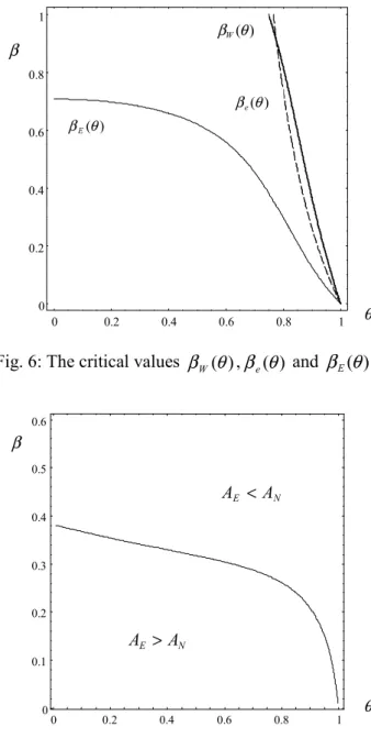
Proposition 4 states that when the compatibility of investments in the case of non-exclusivity dealing is sufficiently low, non-exclusivity is always preferable from a social point of view. The same holds for high degrees of compatibility as long as the bargaining power of the suppliers is sufficiently low. This welfare result is, to a great extent, due to the behavior of the total effective investments. This becomes clear from an inspection of Fig. 6. In Fig. 6, the bold line represents the critical for welfare value of the suppliers' bargaining power, βW(θ). In the area to the left of this line welfare under exclusivity exceeds that under non-exclusivity, while the opposite holds in the area to the right of the line. The dashed line in Fig. 6 represents the critical for the total effective investments value of the supplier's bargaining power, βe(θ). To the left of the dashed line the total effective investments are higher under exclusivity than under non-exclusivity, while the opposite holds to the right of the dashed line. As it can be easily seen the two lines are quite close to each other. Thus, the total effective investments and the social welfare are higher under exclusivity than under non-exclusivity for quite similar parameter configurations.
Having in hand both the buyer’s choice and the welfare comparison we can now answer the following question: does the buyer choose the supply chain structure that is preferable from the social point of view? The answer to this question is not always and it is included in the following statement which is a Corollary of Propositions 3 and 4.
Corollary 1: When 0≤θ ≤0.748 and β >0.707 the buyer chooses non-exclusivity while welfare is higher under exclusivity than under non-exclusivity, the buyer chooses non-exclusivity.
Corollary 1 simply states that there exist cases in which although the buyer chooses non-exclusivity, welfare is not higher under non-exclusivity. In particular, for all the
parameter values between the lines βE(θ) and βW(θ) in Fig. 6, although welfare is higher under exclusivity, the buyer chooses instead non-exclusivity.
From an antitrust policy’s perspective, although our results indicate that the social and the private incentives do not always coincide, they still provide an argument against the view that exclusive dealing is an anticompetitive practice, in the case at least that the exclusivity is initiated by the downstream producers. In fact our welfare analysis shows whenever the buyer chooses exclusivity, welfare is also higher under exclusivity. This can be seen easily in Fig. 6 where the βE(θ) always lies to the left of the βW(θ) line. In other words, there exist no cases in which the buyer’s choice of exclusivity in equilibrium is welfare detrimental.
6. Compatibility of Investments
So far we have assumed that θˆ=1 in the case of exclusivity, while θˆ=θ, with 0≤θ<1, in the case of non-exclusivity. In this section, we relax this assumption by considering a model in which full compatibility can stem as the outcome of an input supplier's strategic choice.
The compatibility between the products of the supplier and the buyer now depends on the supplier's decision to open a specific line of research for the buyer. If a supplier, e.g. supplier S1, opens a specific line of research for B then the compatibility between its investments and those of the buyer is full, θˆ=1, otherwise θ =ˆ θ. Given that sometimes the increase in the compatibility, that is, the opening of a specific line, might be costly, we assume that in order for a supplier to achieve full compatibility with the buyer, it has to incur a fixed cost, denoted by A>0.
In particular, we analyze the same game as in the basic model, modifying it only by decomposing the first stage of the game into two substages, stage 1(a) and stage 1(b). Stage 1(a) is exactly the same as stage 1 of the basic model. In stage 1(b), after the choice among exclusivity and non-exclusivity has been made, each supplier, S1 and S2, simultaneously and independently decides whether or not it will open a specific line of research for B.11
Examining the suppliers' incentives to open a specific line of research both under exclusivity and non-exclusivity, we obtain the following result.
11 We would have obtained qualitatively similar results under an alternative model in which in stage 1(b) the buyer decides how many specific lines it will open given than in the case that it does not open any
θ
Proposition 5: There exist AE >0 and AN >0, with AE > AN when β is sufficiently small, such that (i) under exclusivity the exclusive supplier opens a specific line of research if and only if A< AE, and (ii) under non-exclusivity none of the suppliers opens a specific line of research if A> AN.
Fig. 7 depicts the results included in Proposition 5. In particular, in the area below the curve the critical fixed cost value below which the supplier opens a specific line under exclusivity exceeds the respective critical value above which none of the suppliers opens a specific line under non-exclusivity. The opposite holds in the area above the curve.
It follows from Proposition 5, that there exists a range of values of the fixed cost such that only under exclusivity a supplier opens a specific line for the buyer. Formally:
Corollary 2: If AN < A < AE, then θˆ=1 under exclusivity and θ =ˆ θ under non-exclusivity.
According to Corollary 2 there exists a range of values of the cost of opening a specific research line, such that our basic model with its compatibility assumption can be justified as a reduced form of the more general model analyzed here. It follows that in this range our previous analysis applies.
Finally, it is important to examine whether the cases that the buyer chooses exclusivity in the basic model, correspond to the cases that compatibility can be full only under exclusivity in the extended model. In particular, we know from the basic model that the buyer opts for exclusivity when its bargaining power is sufficiently high, that is, in the area below the βE(θ) curve in Fig. 8. In addition, we know from the extended model analyzed in this section that compatibility could, under some circumstances, turn out to be full only under exclusivity in the area below the
) (θ
βA curve in Fig. 8. It follows that exclusivity with full compatibility could emerge
in equilibrium in the intersection of the areas, provided however that the costs of opening a specific line of research take some intermediate value, that is, provided that .AN < A< AE
7. Conclusions
In this paper, we have considered two distinct supply chain structures, an exclusive supply chain structure and a non-exclusive one. Moreover, we have examined a final
good producer’s choice among these two supply chain structures, in an environment where both sides of the market, upstream and downstream, undertake quality-enhancing investments and bargain over their terms of trade.
We have found that although the compatibility of the buyer’s and supplier’s investments is full only under exclusivity, the investments under exclusivity may not exceed those under non-exclusivity. We have also found that the buyer will opt for exclusivity only when its bargaining power is sufficiently high. This suggests that the observed existence of both exclusive and non-exclusive supply chain structures could be also due to differences in the final good producers’ bargaining positions relative to their input suppliers. When the buyer chooses exclusivity, both the buyer's and the supplier's investments as well as the total effective investments are always higher under exclusivity than under non-exclusivity. However, the opposite is not always true in the case that the buyer chooses non-exclusivity. This means that although the investments play a crucial role in the buyer's decision whether or not it will opt for exclusivity, they are not the only force at work. The buyer's decision is also affected by the fact that the competition among the suppliers is higher in the case of non-exclusivity relatively to that in the case of exclusivity. From a welfare perspective, we have found that there exist no cases in which the buyer’s choice of exclusivity in equilibrium is welfare detrimental. Hence, our results provide an argument against the view that exclusive dealing is an anticompetitive practice, in the cases at least that the exclusivity is initiated by the downstream final good producers.
In sum, we have provided a simple theoretical foundation for the frequently observed buyer initiated exclusive relations in supply chains. Our paper is just a first step towards this direction. In future work we plan to extend our analysis by considering unobservable and/or different degrees of compatibility for the two input suppliers. Moreover, we plan to analyze the strategic incentives for exclusivity in a setting with downstream competition.
Appendix Proof of Lemma 1
Case (a), the case with si = sj≥ 0, cannot be an equilibrium because one of the suppliers
will always have incentives to deviate. In particular, when si = sj = 0 both of the
suppliers have zero profits and one of them has always incentives to deviate and undertake positive investment levels because by doing so it will earn positive profits. Similarly, when si = sj> 0 both of the suppliers make negative profits and one of them
always has incentives to deviate and undertake zero investment levels so that its profits are equal to zero. Given that one of the suppliers will undertake higher investments than the other and thus that it will offer a higher quality input, we can conclude that the supplier with the lower quality input will undertake zero investments, otherwise it will make negative profits.
□
Proof of Lemma 2
We know from Lemma 1 that the equilibrium will take the following form:
) 0 , , ( ) , , ( N i N j i s b s s b = , with i, j =1,2, i≠ j and N >0. i
s W.lo.g. we assume that S1 is
the supplier that undertakes the positive investment levels. In order to find the equilibrium levels of b and s1 we proceed in the following way. We start by assuming that S2 deviates and chooses s2 > s1. If s2 > s1, then in accordance with case (b), in the third stage, w2 = c and the franchise fee with probability β will be equal to:
4 ) ) ( ( 4 ) ) ( ( 2 1 2 2 2 c s b a c s b a F = +θ + − − +θ + − (A1)
The respective expected profits of the deviating supplier will be:
(
) (
)
2 4 ) ( 4 ) ( ) , , ( 22 2 1 2 2 2 1 2 s c s b a c s b a s s b ES − + + − − + + − =β θ θ (A2)From the first order condition of (A2) w.r.t. s2 it follows that the profits of S2 in case of deviation will be maximized by choosing the following level of investments s2:
2 * 2 2 βθ θ βθ − + − = a c b s (A3) In order for S2 not to have incentives to deviate, it is sufficient that s1 is greater or equal to the value of s2 given by equation (A3) above. This is so because when s1 is greater or equal to the above value then the deviation profits of S2 are negative. The last thing for determining the equilibrium in the second stage is to find the levels of investments that
S1 and B choose in order each of them to maximize its profits under the constraint that
* 2 1 s
s ≥ . Formally, S1 and B solve the following maximization problems:
(
)
2 4 ) ( 4 ) ( ) , , ( 2 12 2 1 2 1 1 1 s c b a c s b a s s b E Maxs S − + + − − + − =β θ θ 2 1 2 . . βθθ βθ − + − ≥ a c b s t s(
)
2 4 ) ( 4 ) ( ) 1 ( ) , , ( 2 2 2 1 2 1 b c b a c s b a s s b E Maxb B = −β +θ + − +β +θ − −From the first order conditions of the two maximization problems, we have:
2 1 1 2 1 2 ) 1 ( ) ( ; 2 ) ( θ β θ θ βθ θ βθ − − + − = − + − = a c b b s a c s b s (A4)
Solving the above system of equations, we obtain the investment levels of B and S1
given by equation (9). It is easy to check that these are the equilibrium investment
levels, since the value of s1 given by equation (9) does satisfy the constraint *
2 1 s
s ≥ .
Finally, substituting (9) in the expected net profits of B and S1 we obtain their
equilibrium profits in the non-exclusivity case, given by equations (10) and (11) respectively.
□
Proof of Proposition 1
We differentiate the equilibrium values given by equation (9) with respect to β and our result follows immediately.
□
Proof of Lemma 3
The first order conditions of (18) with respect to s1 and b are:
β β β β + − + − = − − + = 1 ) 1 ( ) ( ; 2 ) ( 1 1 1 c s a s b c b a b s
Solving the above system of equations, we obtain the equilibrium levels of investments given by (19). Finally, substituting these equilibrium values into profit functions of S1
and B, we obtain their equilibrium expected net profits included in equation (20).
□
Proof of Proposition 2
(i) Taking the difference of equations (19) and (9), we have:
1 ) ( − =Κ = − D N c a b bE N b (A5)
where )D=4+β2θ4−2θ2(1+β and ).=4−4β −2θ −2θ2 +β2θ2(2+θ2−βθ2 +θ
b N
The denominator of the above expression, D, is always positive. Regarding the
numerator, ,Nb setting it equal to zero and solving for the critical value of β in terms of
θ, we obtain: 0 3 8 2 4 5 3 2 3 1 ) ( 3 3 4 2 3 2 2 > + − + + + − + − + + = W R W R b θ θ θ θ θ θ θ θ β where R=28+6θ −54θ2 +14θ3 +18θ4 −θ6 −3θ5 and . 24 6 66 21 213 132 516 72 396 48 144− θ − θ2 + θ3 + θ4 − θ5− θ6 + θ8+ θ7 − θ10 − θ9 = W
Next we calculate the difference (A5) at the extreme values of β:
0 2 ) ( ; 0 2 1 ) 2 )( ( 1 2 1 2 1 0 − < − = > − + + − = → → θ θ θθ θ β β c a K lim c a K lim
It follows from the above that K1>0 if and only ifβ <βb(θ).Moreover, differentiating
K1 w.r.t. θ we have: 0 4 4 12 2 4 8 ) ( 2 6 4 4 2 2 2 2 4 3 2 1 =− − + + − + − + < ∂ ∂ D c a K βθ β θ β θ θ β θ β θ θ
Thus, we also have that ∂βb(θ)/∂θ <0 for all values of θ. Finally, in order to show
that ( ) 0
1 =
→ β θ
θ b
lim , we calculate the ( / ).
1 bN bE
lim
→
θ It can be checked that the latter is
strictly increasing in β and that it is equal to zero for β= 0. (ii) Taking the difference of equations (19) and (9), we have:
2 1 ) ( K D N c a s s N s i E− = − = (A6) where =4−2βθ2 −2θ2+β2θ4 −2θ. s N
The denominator of the above expression, D, is always positive. Regarding the
numerator, ,Ns differentiating it w.r.t. β we have: 0 ) 1 ( 2 2 2− < = ∂ ∂ θ βθ βs N
Thus, Ns takes its maximum value when β→ 0 and its minimum value when β→ 1. In
particular: ) 2 2 )( 2 ( ; 0 ) 2 )( 1 ( 2 3 2 1 0 = + + > → = − + − → θ θ β θ θ θ β Ns lim Ns lim
839 . 0 2 33 3 19 4 33 3 19 3 1 3 3 ≈ − + + + = θ Since 0 1 > → Ns lim
β if and only if 0≤θ ≤0.839, it follows that Ns >0 when
839 . 0
0≤θ ≤ for all values of β. Setting Ns equal to zero and solving for the critical value of β in terms of θ, we obtain the following:
2 2 3 2 2 1 ) ( θ θ θ θ βs = − + −
Since we know from the above that when 0.839<θ <1, 0
0 >
→ Ns lim
β and limβ→1Ns <0, it
follows that when 0.839<θ <1, Ns >0 if and only if β <βs(θ). Moreover,
differentiating ).βs(θ w.r.t. θ we have: 0 ) 3 2 2 ( 6 3 2 2 2 3 2 ) ( 2 3 2 2 < − + − − + − + = ∂ ∂ θ θ θθ θ θ θ θθ βs
It follows from the above that βs(θ) takes its minimum value when θ → 1. Since
0 ) ( 1 = → β θ θ s
lim , it follows that βs(θ)>0 when 0.839<θ <1. (iii) Taking the difference of the effective total investments:
3 1 ( ) ( ) K D N c a s b s b N e i N E E + −θ + = − = (A7) where =2(2−2βθ2−2θ2+β2θ4). e N Differentiating K3 w.r.t. θ we obtain: 0 ) 2 2 4 ( ) 1 ( 8 2 4 2 2 2 2 2 3 < + − − − − = ∂ ∂ θ β θ βθθ βθ θ K Moreover, we have: 2 2 4 2 3 1 2 2 3 0 (2 ) ) 4 2 ( 2 ; 0 2 ) 1 ( 2 θ θ θ θθ β β − + − = > − − = → → K lim K lim
The latter is positive if and only if 0≤θ ≤0.766. Thus, when 0≤θ ≤0.766, K3>0. Setting K3 equal to zero and solving for the critical value of β in terms of θ, we obtain the following: 2 2) 2 1 ( 1 ) ( θ θ θ βe = − − +
Since we know from the above that when 0.766<θ <1, 3 0
0 >
→ K lim
β and limβ→1K3 <0, it
follows that when 0.766<θ <1, then we have K3 > 0 if and only if β <βe(θ). Moreover, differentiating βe(θ). w.r.t. θ we have that for 0.766<θ <1:
0 2 1 1 2 1 2 ) ( 2 3 2 2 < + − − + − − = ∂ ∂ θ θ θ θ θθ βe Finally, we calculate ( ) 0. 1 = → β θ θ e lim
□
Proof of Proposition 3Taking the difference of equations (20) and (10), we have the following:
4 2 2 2 ) ( K D N c a E E N E B E B − = − = (A8) where =8+4β2θ4 −16βθ2 +8βθ4 −4β3θ6−12θ2 +4θ4 −4θ6β2 +β4θ8− E N . 5 24 16 4 10 16 12β4θ4 + β3θ2 − β3θ4 + β5θ6 − β2+ β2θ2+ θ6β4 −β6θ8 Differentiating K4 w.r.t. θ we obtain: 0 2 6 ) 1 ( 12 ) 1 ( 8 ) 1 ( 32 ) 1 ( 16 ) ( 3 6 6 5 4 6 2 4 2 2 2 2 2 4 < + − − + + + − − + − − − = ∂ ∂ D c a K β θ β θ β β θ β θ β θ β β θ β θ θ Moreover, we have: ) 2 1 ( 2 1 ; 0 ) 2 2 ( 2 4 2 2 2 ) 2 ( 2 3 0 2 2 2 3 4 4 1 β β β β β β β β β θ θ − + < = − − + + − − = → → K limK lim
The latter is negative if and only if β >1 2 ≈0.707. Thus, when β >0.707,we have
K4 < 0. It is easy to show that ∂K4/∂β <0 when 0<β <0.707. In addition, we have: 0 ) 2 ( 2 ) 1 ( ; 0 ) 2 2 6 16 )( 2 2 ( 2 2 4 0 2 2 4 2 4 2 / 1 − > − = < − − + − = → → θ θ θ θ θ θ β βlim K lim K
It follows that when 0<β <0.707, there exists βE(θ)>0 such that K4 > 0 if and only if )β <βE(θ . Since 0∂K4/∂θ < , we also have that ∂βE(θ)/∂θ <0. Finally, to show
that ( ) 0 1 = → β θ θ E lim , we take ( / ) 1 E B N B E E lim →
θ . It can be checked that the latter is strictly
increasing in β and that it is equal to zero for β = 0.
□
Proof of Proposition 4
) 1 ( ) ( − 2 +β −β2 = a c WE (A9) 2 4 2 2 2 6 4 4 2 2 2 2 2 ) 2 2 4 ( 2 4 4 4 12 ) ( θ β βθ θθ β β θ β θ θ + − − − + − − − = a c WN (A10)
Taking the difference of (A9) and (A10), we have:
4 2 2 ( ) ) ( a c K D N c a W W W W N E − = − = − (A11) where =2(4−2θ2(1+β)+β2θ4)2 >0 W D . 4 ) 1 ( 4 12 ) ) 1 ( 2 4 )( 1 ( 2 +β −β2 − θ2 +β +β2θ4 2 − + θ2 +β2 − β2θ4+β4θ6 = W N
It is to check that K5 >0 when 0≤θ ≤0.748 for all β. Moreover, we have: 0 ) 1 ( 8 5 ; 0 ) 2 2 ( 2 4 6 9 6 2 ) 2 ( 5 0 2 2 2 3 4 5 1 − + < = + − > − − + − − = → → β β β β β β β β β β θ θ K limK lim
In order to define the critical value of β, βW(θ), for 0.748<θ <1, we set NW =0. Taking the total derivative of NW =0, we obtain: dβ /dθ =−(∂NW /∂θ) (∂NW /∂β).
Substituting 0NW = in the latter, one can check, after some manipulations, that it is
always negative. It follows that when 0.748<θ <1, there exists βW(θ)>0 such that
K5 > 0 if and only if β >βW(θ) and that βW(θ) is strictly decreasing in θ.Finally, to
show that ( ) 0,
1 =
→ β θ
θ W
lim we take the ( / )
1 WN WE
lim
→
θ . It can be checked that the latter is
strictly increasing in β and that it is equal to zero for β = 0.
□
Proof of Proposition 5
(i)In the case of exclusivity when S1 opens in stage 1(b) a specific line for B, the continuation of the game is exactly the same as the one included in section 4. Thus, the profits of S1 are given by the difference of equation (20) and the fixed cost A:
A c a EEA S = − − − 2 2 ) ( 2 1 β β (A12) When S1 does not open a specific line for B in stage 1(b), we follow exactly the same procedure as the one included in section 4 with the only difference that we no longer assume that θˆ=1. Doing so, we obtain the profits of S1 when it does not open the specific line: 2 2 2 2 ) 2 ( 2 2 ) ( 1 θ β θ β − − − = a c EEN S (A13)
Taking the difference of equations (A12) and (A13), setting it equal to zero and solving for A, we find: 2 2 2 2 2 2 ) 2 ( 2 2 4 6 ) 1 ( ) ( θβ θ θ β θ β − − + − − − = a c AE (A14)
Since the profits given by equation (A12) are always lower than that given by equation (20), it follows that S1 opens a specific line of research for B, when A < AE.
(ii) In the case of non-exclusivity when none of the suppliers opens a specific line, the analysis is exactly the same as the one included in section 3. Thus, the profits of Sj are
zero while those of Si are positive and are given by equation (10). In order for this to be
the equilibrium, that is, in order none of the suppliers to open a specific line it is sufficient to show that Sj does not have incentives to deviate and open a specific line.
W.lo.g. we assume for the rest of the proof, that in the case where none of the suppliers opens a specific line, S2 is the supplier with the zero profits and S1 is the supplier with the positive profits. In case that S2 deviates and incurs A, then the continuation of the game is similar to that in section 3. The only difference is that the degree of compatibility is now asymmetric for the two suppliers, that is, θˆ=1 for the investments of S2, and θˆ=θ, with 0≤θ<1, for the investments of S1. Next we provide the continuation of the game in the case of deviation. In the fourth stage, the buyer chooses its output in order to maximize its gross profits:
q w q s b a i i B =( +θˆ( + )− − ) π
The equilibrium quantity of the final good is:
2 ) ( ˆ ) , , ( i i i i w s b a s b w q = +θ + −
where the subscript i = 1, 2 indicates the supplier from which the buyer obtains the input. In case it obtains the input from S2, 1θˆ= , while in the case it obtains it from S1,
.
ˆ θ
θ = In the third stage, we distinguish among the following three cases:
(a) b+s2 =θ(b+s1): Similarly to the case with symmetric θˆ we have (wi, Fi) = (c, 0). (b) b+s2 >θ(b+s1): In this case w1 = w2 = c for both suppliers, however while F1 = 0,
F2 with probability β is equal to:
(
) (
)
4 ) ( 4 2 1 2 2 2 c s b a c s b a F = + + − − +θ + −(c) b+s2 <θ(b+s1): In this case w1 = w2 = c for both suppliers, however while F2 = 0,
F1 is with probability 1-β equal to zero and with probability β equal to:
(
) (
)
4 4 ) ( 2 2 2 1 1 c s b a c s b a F = +θ + − − + + −It follows from the above that Lemma 1 holds here too. Next, we analyze the case in which S2 is the supplier that undertakes the positive investment levels. Later on we will show that indeed in equilibrium S2 and not S1 will be the supplier that undertakes the positive investment levels. In order to find the equilibrium levels of b and s2 we proceed in the following way. We start by assuming that S1 deviates and chooses s1 such that
)
( 1
2 b s
s
b+ <θ + , that is s1 >(s2 +b(1−θ)) θ and then we follow the same procedure as the one in the proof of Lemma 2. Doing so, we find the following equilibrium levels of investments: 2 2 2 2 2 2 2 ) 2 ( ) ( θ β βθ βθ βθ β + − − + − = a c sN (A15) 2 2 2 2 2 2 ) 2 2 2 )( ( θ β βθβθ+ β β θ − − − + − = a c bN (A16)
The respective expected net profits of supplier S2 are:
A N c a ENA A S − + − − = 2 2 2 2 2 ) 2 2 ( 2 ) ( 2 βθ β θ β (A17) where =6−β3θ4+2β3θ3−4β2θ −β3θ2 +4β2θ2 +12βθ −4β2θ3 −4βθ2−4β A N . 4 2 2β2θ4 − θ2 − θ +
Setting (A17) equal to zero and solving for A, we find:
2 2 2 2 2 2 ) 2 2 ( 2 ) ( θ β βθ β + − − = a c N AN (A18) It follows that S2 does not open a specific line of research for B, when A > AN.
Finally, taking the difference AE −AN and setting it equal to zero, we can
implicitly define βA(θ). Since it is impossible to get an analytical expression
forβA(θ), in order to show that AE > AN we need to evaluate instead the following
limit: 1 ) 2 )( 3 ( ) 1 )( 3 ( 4 2 2 2 0 + − > + − = → θ θ θ θ β N E A A lim
References
Bensako, D. and Perry, M. (1993), "Equilibrium Incentives for Exclusive Dealing in a Differentiated Products Oligopoly", RAND Journal of Economics, 24, 646-67.
Bernheim, B. and Whinston, M.D. (1998), "Exclusive Dealing", Journal of Political Economy, 106, 64-103.
Bolton, P. and Whinston, M.D. (1993), "Incomplete Contracts, Vertical Integration, and Supply Assurance'', Review of Economic Studies, 60, 121-48.
Dasgupta, S. (1990), ''Competition for Procurement Contracts and Underinvestment'',
International Economic Review, 31, 841-65.
De Meza, D. and Selvaggi, M. (2003), "Please Hold Me Up: Why Firms Grant Exclusive Dealing Contracts", CMPO Working Paper Series N. 03/066.
Grossman, S.J. and Hart, O. (1986), "The Costs and Benefits of Ownership: A Theory of Vertical and Lateral Integration'', Journal of Political Economy, 94, 691-719. Hart, O. and Moore, J. (1988), "Incomplete Contracts and Renegotiation'', Econometrica,
56, 755-85.
Klein, B. (1988), "Vertical Integration as Organizational Ownership: The Fisher Body-
General Motors Relationship Revisited", Journal of Law, Economics and
Organization, 4, 199-213.
Klein, B., Crawford, R.G. and Alchian, A.A. (1978), "Vertical Integration, Appropriable Rents, and the Competitive Contracting Process", Journal of Law and Economics, 21, 297-326.
Marvel, H.P. (1982), "Exclusive Dealing", Journal of Law and Economics, 25, 1-25. Rubinstein, A. (1982), "Perfect Equilibrium in a Bargaining Model", Econometrica, 50,
97-109.
Segal, I. and Whinston, M.D. (2000), "Exclusive Contracts and Protection of Investments'', Rand Journal of Economics, 31, 603-33.
Tirole, J. (1986), "Procurement and Renegotiation'', Journal of Political Economy, 94, 235-59.