School of Economics
UNSW, Sydney 2052
Australia
http://www.economics.unsw.edu.au
ISSN 1323-8949 ISBN 978 0 7334 2449 6Bayesian Covariance Matrix Estimation using a Mixture of
Decomposable Graphical Models
Helen Armstrong, Christopher K. Carter, Kevin K. F. Wong and
Robert Kohn
School of Economics Discussion Paper: 2007/13
The views expressed in this paper are those of the authors and do not necessarily reflect those of the School of Economic at UNSW.
Bayesian Covariance Matrix Estimation using a Mixture
of Decomposable Graphical Models
Helen Armstrong
School of Mathematics, University of New South Wales Sydney, Australia. Christopher K. Carter
CSIRO Mathematical and Information Sciences, Sydney, Australia. Kevin K. F. Wong
The Institute of Statistical Mathematics, Graduate University for Advanced Studies, Tokyo, Japan.
Robert Kohn
Faculty of Commerce and Economics, University of New South Wales, Sydney, Australia.
Summary. Estimating a covariance matrix efficiently and discovering its structure are
im-portant statistical problems with applications in many fields. This article takes a Bayesian approach to estimate the covariance matrix of Gaussian data. We use ideas from Gaussian graphical models and model selection to construct a prior for the covariance matrix that is a mixture over all decomposable graphs, where a graph means the configuration of nonzero off-diagonal elements in the inverse of the covariance matrix. Our prior for the covariance matrix is such that the probability of each graph size is specified by the user and graphs of equal size are assigned equal probability. Most previous approaches assume that all graphs are equally probable. We give empirical results that show the prior that assigns equal probability over graph sizes outperforms the prior that assigns equal probability over all graphs, both in identi-fying the correct decomposable graph and in more efficiently estimating the covariance matrix. The advantage is greatest when the number of observations is small relative to the dimension of the covariance matrix. The article also shows empirically that there is minimal change in sta-tistical efficiency in using the mixture over decomposable graphs prior for estimating a general covariance compared to the Bayesian estimator by Wong et al. (2003), even when the graph of the covariance matrix is nondecomposable. However, our approach has some important ad-vantages over that of Wong et al. (2003). Our method requires the number of decomposable graphs for each graph size. We show how to estimate these numbers using simulation and that the simulation results agree with analytic results when such results are known. We also show how to estimate the posterior distribution of the covariance matrix using Markov chain Monte Carlo with the elements of the covariance matrix integrated out and give empirical results that show the sampler is computationally efficient and converges rapidly. Finally, we note that both the prior and the simulation method to evaluate the prior apply generally to any decomposable graphical model.
KEY WORDS: Covariance selection; Graphical models; Reduced conditional sampling; Vari-able selection
1. Introduction
Estimating a covariance matrix efficiently is an important statistical problem with many applications, such as multivariate regression, cluster analysis, factor analysis, and discrimi-nant analysis; see, for example, Mardia et al. (1979). Such applications are used in the fields of Business, Engineering, and the physical and social sciences. It is also of considerable in-terest to understand the graphical structure of the covariance matrix because it is directly interpretable in terms of the partial correlations of the underlying multivariate distribution. By the graph of the covariance matrix we mean the pattern of nonzero off diagonal elements in the inverse of the covariance matrix, also called the concentration matrix (see Lauritzen 1996, Chapter 5). Estimating a covariance matrix efficiently and understanding its graphi-cal structure are difficult estimation problems because the number of unknown parameters in the covariance matrix increases quadratically with dimension and by the requirement that the estimate of the covariance matrix is positive definite.
There is a large literature of methods that use shrinkage or Bayesian models to improve on the maximum likelihood estimator of the covariance matrix. See, for example, Dempster (1969), Dempster (1972), Efron and Morris (1976), Yang and Berger (1994), Chiu et al. (1996), Giudici and Green (1999), Barnard et al. (2000), Wong et al. (2003) and Liechty et al. (2004). The simulation studies in Yang and Berger (1994) and Wong et al. (2003) show that considerable gains in efficiency are possible.
Dempster (1972) advocates a covariance selection approach to estimate a covariance matrix more efficiently, by which he means setting to zero some of the off-diagonal elements of the concentration matrix. His idea is that a more parsimonious model will give greater efficiency. However, the selection of which elements to set to zero is difficult even for moderate dimensions because a p×p concentration matrix has p(p−1)/2 distinct off-diagonal entries and there are 2p(p−1)/2 possible graphs associated with it. Drton and Perlman (2004) give a model selection approach based on simultaneous confidence intervals to determine which partial correlations are zero. The simultaneous confidence intervals are based on large sample theory and become large when pis moderate to large. Drton and Perlman (2004) do not attempt to estimate the covariance matrix based on their selected graph.
A number of articles take a Bayesian approach to covariance selection. For the case of decomposable graphs, Dawid and Lauritzen (1993) introduces a conjugate prior for the covariance matrix called the hyper inverse Wishart distribution. Giudici (1996) uses a prior for the covariance matrix that is a mixture of fixed parameter hyper inverse Wishart priors over decomposable graphs and calculates the marginal likelihood for each decomposable graph. The marginal likelihood is used to calculate the posterior probability of each graph. This gives an exact solution for small examples, but forpgreater than approximately 8 the number of graphs is prohibitively large.
Roverato (2000) shows that the hyper inverse Wishart prior for the covariance matrix is equivalent to a constrained Wishart prior for the concentration matrix. It is straightforward to define a constrained Wishart prior for general graphs, however, such distributions have normalizing constants that are not available analytically unless the graph is decomposable. Roverato (2002), Dellaportas et al. (2004) and Atay-Kayis and Massam (2005) propose effi-cient simulation and importance sampling methods for estimating the normalizing constants for the nondecomposable graphs. The normalizing constants are used to examine a small
number of graphs and select those that that have the highest marginal likelihood or pos-terior probability, rather than to estimate the covariance matrix by averaging over graphs. However, such an approach seems unsuitable as the basis of a Markov chain Monte Carlo sampling scheme whenp is moderate to large because there are 2p(p−1)/2 possible graphs with only a small fraction of them being decomposable.
Giudici and Green (1999) give a MCMC approach that can deal with large values ofp. Their method applies to a hierarchical model with a hyper inverse Wishart prior for the covariance matrix conditional on a decomposable graph. They use reversible jump Metropolis-Hastings methods to generate the covariance matrix and other parameters. Their method has a local computation property that only requires Cholesky decompositions of the submatrix of the covariance matix corresponding to a clique of the graph. Brooks et al. (2003) modify the reversible jump MCMC proposal of Giudici and Green (1999) and give empirical results to show this improves the convergence rate.
Wong et al. (2003) also use MCMC methods to select which off-diagonal element to set to zero. They use reversible jump Metropolis-Hastings methods to generate the inverse covariance matrix and other parameters. The main difference between Giudici and Green (1999) and Wong et al. (2003) is that Wong et al. (2003) do not constrain the possible graphs to be decomposable. Wong et al. (2003) use a prior with normalizing constants based on graph size to avoid having to calculate normalizing constants for each nondecomposable graph. They also need to run a separate MCMC to estimate the normalizing constants for each graph size.
For longitudinal data, Smith and Kohn (2002) factor the concentration matrix using a Cholesky decomposition and carry out variable selection on the strict lower triangle of the Cholesky to obtain parsimony. Their approach is attractive when there is some natural ordering of the observation vector, but there are two potential drawbacks to the Cholesky approach when such a natural ordering does not exist. First, different orderings of the vari-ables can yield different estimates of the covariance matrix. Second, under some orderings the Cholesky factor may be quite full even if the concentration matrix is sparse.
In this paper we consider Bayesian estimation of decomposable covariance selection models, also known as decomposable graphical Gaussian models. Our article makes the following contributions. First, we propose a prior for the covariance matrix such that the probability of each graph size is specified by the user, whereas most previous approaches, e.g. Giudici and Green (1999), assume that all graphs are equally probable. We show by simulation that the prior that assigns equal probability over graph sizes outperforms the prior that assigns equal probability over all graphs, both in identifying the correct decomposable model and in estimating the covariance matrix more efficiently. This advantage is greatest when the number of observations is small relative to the dimension of the covariance matrix. We also show by simulation that there is minimal change in statistical efficiency in using our mixture prior compared to the estimator of Wong et al. (2003), even when the graph of the covariance matrix is nondecomposable.
Our prior requires knowing the number of decomposable graphs for each graph size. The second contribution of the article is to give a MCMC method for estimating these counts. and to show that the counts obtained by the simulation method agree with analytic results when such results are known.
a reduced conditional MCMC sampler for decomposable graphical models, where the co-variance matrix is integrated out of all conditional distributions and is not generated in the MCMC. Our approach does not require reversible jump Metropolis-Hasting methods and has the local computation properties of the Giudici and Green (1999) approach, so the computational complexity for one iteration of our approach is similar to that of Giudici and Green (1999). We expect that our sampler has a faster convergence rate to that of Giudici and Green (1999) and Brooks et al. (2003), but we have not compared them emprically. We show that our sampler has a faster convergence rate than the Wong et al. (2003) approach. A comparison between the MCMC methods described in this paper and a stochastic search approach for finding the graph with maximum posterior probability is the subject of a forthcoming paper (Jones et al. (2005)).
The results in our article suggest that at present there is no ‘best’ method for estimating Gaussian covariance selection models. While the method of Wong et al. (2003) works in principle for all graphs, the convergence of their MCMC simulation can be slow if the true graph has full subgraphs of size 5 or larger because Wong et al. (2003) generate the elements of the concentration matrix one at a time. On the other hand the sampling scheme for decomposable graphs presented in our article is extremely efficient because the concentration matrix is integrated out and is an attractive alternative to the Wong et al. (2003) model for high dimensional graphs that are likely to have substantial full subgraphs. There are two other advantages of the decomposable prior considered in our article. The first is that there is a separate normalizing constant for each decomposable graph, whereas Wong et al. (2003) have a normalizing constant for each graph size. The second is that the Wong et al. (2003) model does not at present allow for hyperparameters in the prior. For example, using an equicorrelated prior as in Giudici and Green (1999) is not at present feasible with the approach of Wong et al. (2003).
The paper is organized as follows. Section 2 briefly introduces graphical Gaussian models. Section 3 describes our Baysian covariance selection model and Section 4 describes our MCMC approach to estimating this model. Section 5 compares the prior that assigns equal probablity to each graph size to the prior that assigns equal probability to each decomposable graph. Section 6 shows how to estimate the number of decomposable graphs for each size by simulation. Section 7 compares the prior that assigns equal probability to each graph size to the prior of Wong et al. (2003). There are two appendices. The first gives the proofs of the results in the paper. The second gives a computationally efficient expression for evaluating the ratio of normalizing constants from Section 4.1.
2. Background on Gaussian graphical models
Before explaining our Bayesian covariance selection model we provide some background on Gaussian graphical models. Further details on such models are available in Dawid and Lauritzen (1993) and Chapters 2, 3 and 5 of Lauritzen (1996).
Let g = (V, E) be an undirected graph with vertices V = {1, . . . , p} and set of edges
E⊆V×V. For a square matrixAwe writeA >0 to denote thatAis positive definite. Let
M+(g) be the set ofp×pmatrices Ω satisfying Ω>0 and Ωij = 0 for all pairs (i, j)∈/ E. For a givenp×pcovariance matrix Σ, we define the graph of Σ, g =g(Σ) = (V, E), as follows. Let Ω = Σ−1. LetV ={1, . . . , p}and define E={(i, j), i=j such that Ωij = 0}.
Thus the graphg=g(Σ) gives the configuration of nonzero off-diagonal elements in Ω. We say that an m×m matrix A > 0 has an inverse Wishart (IW) density with δ > 0 degrees of freedom and scale matrix Φ, denoted asA∼IW(m, δ,Φ),if the density ofAis
p(A|δ,Φ) = | Φ 2| δ 2 Γm(δ2)| A|−(δ+m2+1)etr −1 2ΦA −1, (1)
where etr(A) = exp(trace(A)) and forα > (m−21),
Γm(α) =πm(m−1)/4 m i=1 Γ(α−(i−1 2 )) is the multivariate gamma function (Muirhead, 1982, p. 113).
Lauritzen (1996, Definition 2.3, p.8) defines adecomposable graph and we refer to a covari-ance matrix Σ as decomposable if its graphg=g(Σ) is decomposable.
Suppose that g is a decomposable graph and let C1, . . . , Ck be a perfect sequence of the cliques ofg. LetHj=C1∪. . .∪Cj be the history of the sequence and letSj =Hj−1∩Cj be the separators forj= 2, . . . , k. For any matrixM and subset of verticesB, useMBBto denote the symmetric submatrix ofM which is formed by taking every corresponding entry
Mij for which the vertices{Vi, Vj} ∈B. Using the parameterization of Dawid (1981), we say Σ has ahyper inverse Wishart(HIW) distribution, withhyperparameters (δ,Φ) denoted by Σ∼HIW(g, δ,Φ), if for Σ−1∈M+(g) p(Σ|δ,Φ, g) = k i=1 p(ΣCiCi|δ,ΦCiCi) k i=2 p(ΣSiSi|δ,ΦSiSi) , (2)
whereδ >0, Φ>0, and the density is with respect Lebesgue measure on the elements of Σ corresponding to edges ofg.
In (2), the termsp(ΣCiCi|δ,ΦCiCi) denote the IW densities ΣCiCi∼IW(|Ci|, δ+|Ci| −1,ΦCiCi) given by p(ΣCiCi|δ,ΦCiCi) = ΦCiCi 2 δ+|Ci|−1 2 Γ|Ci| δ+|Ci|−1 2 |ΣCiCi| − δ+2|Ci| 2 etr −1 2(ΣCiCi) −1Φ CiCi , (3)
where |Ci| denotes the cardinality of the clique Ci, and the terms p(ΣSiSi|δ,ΦSiSi) are defined similarly. Note that the expression in (2) is invariant to the choice of perfect sequence.
From (1) – (3), the normalizing constant for the HIW distribution is
h(g, δ,Φ) = k i=1 ΦCiCi 2 (δ+|Ci|2 −1) Γ|Ci| δ+|Ci|−1 2 −1 k i=2 ΦSiSi 2 (δ+|Si|2 −1) Γ|Si| δ +|Si|−1 2 −1. (4)
3. Bayesian Covariance Selection models
3.1. Likelihood and hierarchical structure
Suppose we have independent observations
yt∼N(µ,Σ), t= 1,· · · , n, (5) whereytis p×1.Lety = (y1,· · · , yn) be the data. We use a hierarchical prior forµ and Σ of the form
p(µ,Σ,Φ, δ, g) =p(µ|Σ,Φ, δ, g)p(Σ|Φ, δ, g)p(Φ|δ, g)p(δ|g)p(g),
where each of the terms on the right is discussed below. In our article we assume that
p(µ|Σ,Φ, δ, g)∝ constant, as our focus is on priors for Σ.The prior for Σ depends on its graphg, the p×pmatrix Φ and the scalarδ, and is is discussed in Section 3.2. Section 2 defines the graph of Σ as the configuration of nonzero off diagonal elements in Σ−1. The prior for Φ is discussed in Section 3.3 and the prior for the graphgis discussed in Section 3.4. In the article we restrict the graph of Σ to be decomposable, so that the prior for Σ is a mixture over all decomposable graphs. We explain in Section 2 that this is equivalent to the prior for Ω = Σ−1 being a mixture over all Wishart distributions constrained to decomposable graphs.
3.2. Prior forΣ
We use the HIW prior (2) for Σ|Φ, δ, g, which allows Σ to be integrated out in the sampling scheme described in Section 4. Thus, our prior
p(dΣ|Φ, δ) = g
p(dΣ|g,Φ, δ)p(g)
is a mixture of HIW distributions over all decomposable graphs g As discussed in the introduction, Roverato (2000) shows that the inverse of a HIW random matrix has a Wishart distribution, subject to the constraints imposed by the corresponding graph. Thus
p(dΣ|Φ, δ) = g
p(dΣ|g,Φ, δ)p(g)
is a mixture of of constrained Wishart distributions over all decomposable graphs.
In our article we set the degrees of freedom parameterδ to 5 as such a value ofδ gives a suitably noninformative prior for Σ.
3.3. Prior specification forΦand its parameters
We consider the following three specifications for the hyperparameter Φ, and refer to them as the hyperprior forms of Φ:
(b) Φ =τ(ρJ+ (1−ρ)I), τ >0 whereJ is thep×pmatrix of ones andρis a correlation coefficient that needs to be in the open interval (−1/(p−1),1) for Φ to be positive definite. This specification is used by Giudici and Green (1999) and is called the
equicorrelated version of Φ because Φii =τ and Φij=τ ρfori=j. (c) Φ =τ Sy/(n−1),whereτ >0, Sy= n t=1 (yt−y)(yt−y), (6) andy is the mean of theyt.
We motivate the choice of Φ in two ways. First, by integrating µ out of p(y|µ,Σ), withp(µ) constant, we obtain
p(y|Σ)∝ |Σ|−(n−1)/2etr
−1
2SyΣ
−1. (7)
Suppose g is a decomposable graph. If we take p(Σ|g)∝ p(y|Σ)1/(n−1), then from (7) and equation (3) of Giudici (1996), we can write p(Σ|g) in the form (3) with Φ =Sy/(n−1).
A second motivation for this choice of Φ is to note that if Σ∼ HIW(p, δ,Φ), then
E(ΣCC) = ΦCC/(δ−2) for any clique C = Ci or separator C = Si in (2). Since (Sy)CC/(n−1) is an unbiased estimator of ΣCC, this suggests taking Φ∝Sy/(n−1). We assume in all cases thatτis uniform on the interval [0,Γ] where Γ is large, e.g. Γ = 1010, and in the equicorrelated case thatρis uniform on the open interval (−1/(p−1),1).
3.4. Prior forg
We first define notation for theedge indicators of a graphg. Let
eij =
1 if (i, j)∈E
0 otherwise (8)
and lete−ij ={ekl: (k, l)= (i, j)}.Note that any graphg= (V, E) can be unambiguously written asg= (eij, e−ij).
For a given graphg=g(Σ), let the number of edges, or thesize ofg, be given by
size(g) = i<j
eij (9)
i.e. size(g) is the number of nonzero elements in the strict upper triangle of Ω, andsize(g)≤
r=p(p−1)/2.
Because of the theoretical and practical difficulty in calculating for a given p the exact number of decomposable graphs, or the number of graphs of a given size, most of the literature for both decomposable and general models takes the prior forg as uniform over all the relevant graphs; see, for example, Giudici and Green (1999), Dellaportas and Forster (1999), Geiger and Heckerman (2002), Giudici and Castelo (2003), Roverato (2002), and Atay-Kayis and Massam (2005).
Such a prior favours any class of graphs with many members over a class with few members, and favours middle sized graphs over both very large and very small sized graphs.
LetAp,k denote the number of graphs of sizek. We specify the prior for a graphg hierar-chically as follows.
p(g|size(g) =k) = 1
Ap,k,
so that all graphs of a given size are equally likely. We now specify the prior for the size of a graph. One choice is
p(size=k)∝Ap,k, which means that
p(g) =p(g, size(g)) =p(g|size(g))p(size(g))∝constant,
giving the uniform prior forg. A more flexible prior is of the form
p(size=k|ψ) = r k ψk(1−ψ)r−k,
where we interpret ψ as the probability that any two vertices have a common edge. We could then put a prior onψ. Suppose we take the prior forψas a beta with parametersa
andb, i.e. p(ψ) =ψ a−1(1−ψ)b−1 B(a, b) . Then, p(size=k) = r k B(a+k, r−k+b) B(a, b) and p(g) =p(g|size(g))p(size(g)) (10) = r size(g) B(a+size(g), r−size(g) +b) Ap,size(g)B(a, b) , (11)
whereB(a, b) is the beta function. We could now also put a prior ona, b. In our article we takeψuniform so thata=b= 1, which means that
p(size=k) = 1
(r+ 1) and p(g) = 1 (r+ 1)Ap,k .
That is, the size of each graph has equal probability, and the probability of a graph of size
kconditional onsize=kis uniform. However our framework is more flexible than this. We call this the size based prior forg and compare results against those using a uniform prior.
The size based prior makes it easier to discover sparse and full graphs whenn/p is small. The countsAp,k are not available in the literature. Section 6 gives results to calculate a subset of them analytically, and shows how to evaluate the rest by simulation.
4. Posterior inference and Markov chain Monte Carlo sampling
We use Markov Chain Monte Carlo (MCMC) simulation to obtain all posterior distributions. The simulation involves the generation of the graphsg and the parameters in Φ but not Σ andµwhich are integrated out. Thus, our sampling scheme is said to generate fromreduced conditionals and is therefore expected to be more efficient than the sampling schemes in Giudici and Green (1999) and Wong et al. (2003) that generate Σ as part of their sampling scheme.
We note that iterates ofµand Σ can also be generated in conjunction with the simulation, but such iterates ofµ and Σ do not have any influence on the convergence properties or dependence structure of the reduced conditional simulation.
The following theorems are useful in evaluating the conditional distributions required in the simulations. The first theorem gives a conjugate prior property of the HIW distribution. LetSy be defined by (6) and define
Φ∗= Φ +Sy andδ∗=δ+n−1 . (12) Theorem 1. (Dawid and Lauritzen, 1993) For the Bayesian model specified by (2) and (7)
Σ|y, δ,Φ, g∼HIW(g, δ∗,Φ∗).
Proof. See Dawid and Lauritzen (1993) or Appendix A.
The next theorem gives an expression for the marginal likelihood.
Theorem 2. (Giudici, 1996) For the Bayesian model specified by (2) and (7),
p(y|δ,Φ, g) = (2π)−((n−1)p/2) h(g, δ,Φ)
h(g, δ∗,Φ∗) (13)
Proof. See Giudici (1996) or Appendix A .
4.1. Sampling the graphs g
We sample the graphsgby generating the edge indicators one at a time, conditional onδ,Φ ande−ij ={ekl,(k, l)= (i, j), k < l}using the following MH sampling scheme.
Using the notation of Section 3, let gc = (V, Ec) be the current graph of Σ, which is decomposable by construction with edge indicators{eckl: 1≤k < l≤p}.
We choose a pair (i, j) at random and suppose that g = (eij, ec−ij) is decomposable for botheij = 0 and eij = 1.We use the legal edge addition and deletion characterizations of Giudici and Green (1999) and Frydenberg and Lauritzen (1989) respectively to ensure this. Otherwise we choose a new pair (i, j).
Set the proposal graph asgp (conditional ongc) asg= (epij, ec−ij) whereepij= 1−ecij. This means that the proposal density foreij isqg(a|b, ec−ij) whereaandbare each either 0 or 1, andqg(a= 1−b|b, ec−ij) = 1.
The MH acceptance probabilty for the proposal is min 1,p(y|g p,Φ, δ) p(y|gc,Φ, δ) p(gp) p(gc) (14)
becauseqg(ecij|eijp, ec−ij)/qg(epij|ecij, ec−ij) = 1. The ratiop(gp)/p(gc) is known and the ratio of marginal likelihoods p(y|gp,Φ, δ) p(y|gc,Φ, δ) = h(gp, δ,Φ) h(gc, δ,Φ) h(gc, δ∗,Φ∗) h(gp, δ∗,Φ∗). (15)
A simple expression for (15) is derived in Appendix B.
4.2. Generating the parameters inΦ
In all cases of Section 3.3 we generateτ using a random walk MH method
log(τp) = log(τc) +ξτ , ξτ ∼N(0, στ2), which has acceptance probability
min 1,p(y|g, τ p, ρ) p(y|g, τc, ρ) p(τp) p(τc) (16)
as the proposal densities cancel out. In the equicorrelated case, the parameterρis generated similarly toτ by a random walk MH method
ρp=ρc+ξρ , ξρ∼N(0, σρ2).
The choice of the variancesστ2, σ2ρ is sensitive top, and was fine tuned to attain acceptance probabilities of around 25% according to the acceptance rate of the proposals. For the case
p= 17 reported in this paper, such an acceptance probability resulted from usingστ2= 1/10 andσρ2= 1/20.
4.3. GeneratingΣ,Ωandµ
Althoughµ,Σ and Ω are not generated in the MCMC simulation, it is often necessary to estimate functionals of µ,Σ and Ω. Such functionals can be estimated by sampling from the posterior distribution of Σ,Ω andµ. Conditional on (g, δ,Φ) it follows from Theorem 1 that p(Σ|y, g, δ,Φ) is HIW (δ+n−1,Φ +Sy) so that Σ and Ω can be generated using Theorems 3 and 4 of Roverato (2000). It is straightforward to show thatp(µ|y,Σ, g, δ,Φ) is
N(y,Σ/n), and hence to generateµ, giving iterates{µ[j],Σ[j],Ω[j], j≥1}from the posterior distribution.
4.4. Efficient estimation ofE(Ω|y)
The posterior mean of Ω is not only used as an estimator of Ω, but also of Σ because
of estimatingE(Ω|y) is to use the histogram estimatorJ−1Jj=1Ω[j]. A statistically more efficient estimator is the mixture estimatorJ−1Jj=1E(Ω|y, g[j], δ[j],Φ[j]).
We now show how to efficiently compute E(Ω|y, g, δ,Φ) using the following notation from Lauritzen (1996). Suppose thatAis a p×pmatrix and S ⊂V. Let B = [ASS]V be the
p×pmatrix defined by
Bij=
Aij if{i, j} ⊂S 0 otherwise
Theorem 3. Suppose thatΩ|y ∼W(g, δ∗,Φ∗), where g is decomposable. Then, using the notation of this and Section 3,
E(Ω|y, δ,Φ, g) = k i=1 (δ∗+|Ci| −1)Φ∗CiCi −1V − k i=2 (δ∗+|Si| −1)Φ∗SiSi −1V . (17)
Proof. See Appendix A.
5. Comparison of the size prior for a graph with the uniform prior
This section compares the prior based on the graph size with the uniform prior that is used in most previous articles. Performance is in terms of a loss function and a simulation was carried out to numerically assess performance. We found that overall the size based prior forgoutperformed the uniform prior.
Our simulation considered the following five graph types for g. (a) Ω = I, the identity matrix, representing the empty graph and a diagonal covariance matrix; (b) Ω tridiagonal, representing a sparse and decomposable graph (this is a chain graph with p−1 edges); (c) Ω an ‘extreme’ full matrix (the correlation coefficients ρij of Ω−1 satisfy |ρij| > .30), which is a complete graph; (d) Ω corresponding to a 4-cycle on p vertices representing a sparse but nondecomposable graph; and (e) Ω corresponding to a p−cycle on pvertices, again representing a sparse but nondecomposable graph. We note that the nondecomposable graphs in (d) and (e) require the addition of extra edges when we estimate them by a mixture of decomposable graphs. Furthermore, (e) is an extreme case of non-decomposability, as it requires a minimum ofp−3 fill ins. Conversely, the unchorded 4-cycle onpnodes requires the fewest number of fill ins, so was chosen as an indicator of performance for the sparsest nondecomposable case.
The simulation considered the three forms of Φ described in Section 3.3 and two sample sizesn= 40 andn= 100. We report results for matrices of sizep= 17, but similar results were obtained for matrices of other sizes.
Let ΣT be the true value of Σ and letΣ be an estimator of Σ T. We measure the performance ofΣ using the L1loss function
L1(Σ,ΣT) = trace(ΣΣ T−1)−log det(ΣΣ −T1)−p. (18) This loss function is frequently used to compare estimates of the covariance matrix, e.g. Yang and Berger (1994). It is straightforward to show thatL1≥0 for allΣ and Σ T, and that it
is only equal to 0 ifΣ = Σ T. It is also straightforward to show that fory∼N(0,Σ), L1(Σ,ΣT) =− p(y|Σ) log p(y|ΣT) p(y|Σ) dy (19)
i.e. L1is equivalent to a Kullback-Liebler distance betweenp(y|ΣT) andp(y|Σ) with respect to the densityp(y|Σ). The Bayes estimator for Σ for the L1loss function isE(Ω|y)−1, which can be computed as in Section 4.4.
We use boxplots to compare replication by replication the size based prior with the uniform prior in terms of the percentageincrease in the loss function L1 resulting from using the uniform prior compared to the size-based prior; i.e. the boxplots are based on calculating
100(Lunif1 −Lsize1 )/Lsize1
for each replication, whereLunif1 andLsize1 are the values ofL1(Σ,ΣT) for the uniform and size based priors respectively.
The boxplots are based on 20 replications with each replication consisting of 2,000 burnin iterations and 20,000 sampling iterations. We ran the sampler for the casep= 17 onn= 40 and 100 observations from five simulated data sets corresponding to the five models (a)–(e) for Ω.
Figure 1 presents the results forp= 17. The plots show that for Φ =τ I and Φ equicorre-lated, the size prior is at least as good, and often much better than, the uniform prior. For Φ =τ Sy/(n−1), the comparison between the size prior and the uniform prior is inconclu-sive forn= 40, but forn= 100 the size prior is at least as good as, and often better than the uniform prior. We conclude that the size based prior outperforms the uniform prior. We also compared the performance of the three forms of Φ for the uniform and size priors and found that overall the equicorrelated form of Φ using the size based prior for the graph performed best, and it is this combination that we use for the rest of the paper.
6. Evaluating the size based prior
To use the size based prior for graphs on p vertices, we need the set of numbers {Ap,k :
k= 0, . . . , r}whereAp,k is the number of decomposable graphs of sizekonpvertices, and
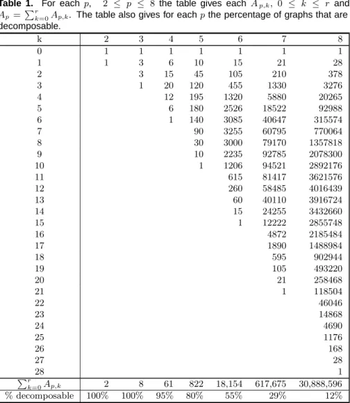
r=p2is the maximum graph size. These numbers are not in the literature, nor is there a general method available for computing them. In this section we present some exact values ofAp,kas well as a simulation method that can estimate theAp,k as precisely as necessary. LetBp,k be the number of connected decomposable graphs of size kon pvertices. Equa-tions (3) and (4) of Castelo and Wormald (2001) give recurrences to calculate Ap,k from the Bp,k analytically, and the information to calculate all Bp,k analytically is implicit in Wormald (1985). Forp≤8, Wormald (1985) gives theBp,k from which we computed the
Ap,k and these are reported in Table 1.
However, Wormald’s (1985) analytic approach for obtaining the Bp,k is likely to be com-putationally intractable for p > 25 (private correspondence with Wormald) and even for 8< p≤25 obtaining the Bp,k would take weeks on realistically sized computers. Further-more, analytically deriving theAp,k from theBp,kis computationally feasible only for small
Table 1. For each p, 2 ≤ p ≤ 8 the table gives eachAp,k, 0 ≤ k ≤ r and Ap =rk=0Ap,k. The table also gives for eachpthe percentage of graphs that are
decomposable. k 2 3 4 5 6 7 8 0 1 1 1 1 1 1 1 1 1 3 6 10 15 21 28 2 3 15 45 105 210 378 3 1 20 120 455 1330 3276 4 12 195 1320 5880 20265 5 6 180 2526 18522 92988 6 1 140 3085 40647 315574 7 90 3255 60795 770064 8 30 3000 79170 1357818 9 10 2235 92785 2078300 10 1 1206 94521 2892176 11 615 81417 3621576 12 260 58485 4016439 13 60 40110 3916724 14 15 24255 3432660 15 1 12222 2855748 16 4872 2185484 17 1890 1488984 18 595 902944 19 105 493220 20 21 258468 21 1 118504 22 46046 23 14868 24 4690 25 1176 26 168 27 28 28 1 r k=0Ap,k 2 8 61 822 18,154 617,675 30,888,596 % decomposable 100% 100% 95% 80% 55% 29% 12%
tauI equi tauS 0
200 400
identity
tauI equi tauS
−40 −20 0 20 40 tridiagonal
tauI equi tauS
0 100 200 300
full
tauI equi tauS
0 100 200
4cycle
tauI equi tauS
−50 0 50 100
neqcycle
tauI equi tauS
50 100 150 200 250
tauI equi tauS
0 20 40
tauI equi tauS
0 50 100
tauI equi tauS
0 50 100 150
tauI equi tauS
−50 0 50 100
Fig. 1. Percentage increase in loss of uniform prior relative to the size prior measured underL1loss. The left panels correspond ton= 40and the right panels ton= 100. tauI, equi and tauS correspond toΦ =τI,Φequicorrelated andΦ =τSy/(n−1).
p. Because of these difficulties we propose a simulation methodology to estimate the Ap,k for allp.
6.1. Methodology
We begin with some exact results which can be used to calculate{Ap,k: k≤5 andr−2≤
k ≤ r} analytically for any p. Let Fp,k denote the number of nondecomposable graphs havingpvertices and kedges.
Lemma 4. (a) Ap,k =kr−Fp,k. (b) Fp,0=Fp,1=Fp,r= 0, p≥0.
(c) Fp,2=Fp,r−1= 0, p≥2.
(d) Fp,3= 0, p≥3.
Lemma 5. (a) Forp≥4, Fp,4=p4×3. (b) For p≥4, Fp,r−2=Fp,4.
(c) For p≥5, Fp,5=p5×12 +p4×3×(r−6).
Proof. See Appendix A.
We now show how to estimate the{Ap,k: 6≤k≤r−3}for allp. Our approach is to run a separate simulation to estimate eachAp,k for 6≤k≤r−3. The simulations are done in ascending order ofk, i.e. k= 6, . . . , r−3, and the simulation to estimate a particularAp,k is restricted to graphs of size ≤k and uses the estimates Ap,j of Ap,j forj = 6,· · ·, k−1 that have been calculated in previous simulations.
We now describe the details of the simulation to estimate a particularAp,k. Letφp,k be the initial estimate ofAp,k given by
φp,k=αp,k A2p,k−1 Ap,k−2 (20)
withαp,k chosen in the range (0.5,1). To justify this choice ofφp,k, we note that we have found empirically that logAp,k is approximately a negative quadratic (see figures 2 and 3) so that logAp,k−2 logAp,k−1+ logAp,k−2≤0, and hence
αp,k = Ap,k/Ap,k−1
Ap,k−1/Ap,k−2 ≤1.
We have also found empirically thatαp,k is likely to exceed 0.5. As
Ap,k=αp,k
A2p,k−1 Ap,k−2
the above discussion suggests the choice of φp,k in (20). Further details on the choice of
αp,k can be obtained from the authors.
We use Lemmas 4 and 5, the estimates Ap,j of Ap,j for j = 6,· · ·, k−1 that have been calculated in previous simulations, and the initial estimateφp,kofAp,kgiven above to define the following probability distribution pe(g) on the graphs g of size ≤k. To simplify the notation we omit subscripts forpandkin pe(g).
pe(g)∝ 1 Ap,size(g) if 0≤size(g)≤5 1 Ap,size(g) if 6≤size(g)≤k−1 1 φp,k if size(g) =k (21)
which implies that
pe(size=k) pe(size≤5) = Ap,k/φp,k 5 j=0Ap,j/Ap,j =1 6Ap,k/φp,k
and hence
Ap,k= 6φp,kpe(size=k)
pe(size≤5).
By running the simulation described below based on pe(g) we can estimate the ratio
pe(size=k)/pe(size≤5) by their relative frequencies and hence obtain an estimate of
Ap,k= 6φp,kpˆe(size=k) ˆ
pe(size≤5),
where ˆpe(size=k) and ˆpe(size≤5) are the empirical relative frequencies.
The simulation uses the following MCMC sampling scheme. As in Section 4.1, we generate the edge indicators one at a time conditional on the other edge indicators. Letgc= (V, Ec) be the current graph with edge indicators given by{ekl : (k, l)∈Ec}. We select an edge (i, j) at random. If g = (eij, ec−ij) corresponds to a decomposable graph of size ≤ k for both eij = 0 and eij = 1 then we proceed, where we again use the legal edge addition and deletion characterizations of Giudici and Green (1999) and Frydenberg and Lauritzen (1989) respectively to test this. Otherwise we select a new edge. If we proceed, then we propose a new graphgp= (1−ecij, ec−ij) and accept this graph with probability
min{1, pe(gp)/pe(gc)} which is evaluated using (21).
We note that at each stage we can also re-estimateAp,j, j= 6,· · · , k−1.
6.2. Results
This section presents the estimatesAp,k fork= 0· · ·r andp= 8 and 34. We also provide a general method to check on the quality of these estimates. We note that the prior
pe(g)∝
1
Ap,size(g) if 0≤size(g)≤5 orr−2≤size(g)≤r
1
Ap,size(g) if 6≤size(g)≤r−3
should havepe(size=k) close to uniform and hence close to the target value of 1/(r+1), and that an approximate lower bound for the standard error of the estimates ofpe(size=k) is π(1−π)/J, where π = 1/(r+ 1) and J is the number of iterates used to compute
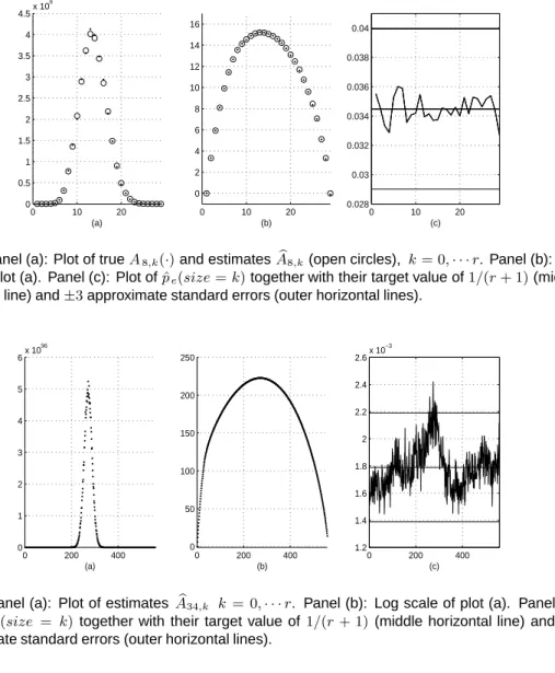
pe(size = k). Our simulations use a burnin period of 2,000 iterations and a sampling period ofN = 10,000 iterations. Figure 2 plots the estimatesAp,k forp= 8 and the true valuesA8,k,k= 0· · ·ron both an absolute and logarithmic scale. Figure 2 also plots the estimates ofpe(size=k) together with the target value 1/(r+ 1) and lower bounds for the
±3 standard error lines.
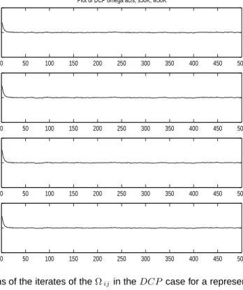
Figure 3 has the same interpretation as Figure 2 but is forp= 34. The true values ofA34,k are not plotted as they are mostly unknown.
For p = 9,· · ·,12 the totals Ap = jAp,j are known, but not the Ap,j. As a further check on results we compared our estimated values of Ap to Ap and found that we were consistently within 1% of the truth.
0 10 20 0 0.5 1 1.5 2 2.5 3 3.5 4 4.5x 10 6 (a) 0 10 20 0 2 4 6 8 10 12 14 16 (b) 0 10 20 0.028 0.03 0.032 0.034 0.036 0.038 0.04 (c)
Fig. 2. Panel (a): Plot of trueA8,k(·)and estimatesA8 ,k(open circles), k= 0,· · ·r. Panel (b): Log scale of plot (a). Panel (c): Plot ofpˆe(size=k)together with their target value of1/(r+ 1)(middle horizontal line) and±3approximate standard errors (outer horizontal lines).
0 200 400 0 1 2 3 4 5 6x 10 96 (a) 0 200 400 0 50 100 150 200 250 (b) 0 200 400 1.2 1.4 1.6 1.8 2 2.2 2.4 2.6x 10 −3 (c)
Fig. 3. Panel (a): Plot of estimates A34 ,k k = 0,· · ·r. Panel (b): Log scale of plot (a). Panel (c): Plot ofpˆe(size = k)together with their target value of 1/(r+ 1)(middle horizontal line) and ±3
approximate standard errors (outer horizontal lines).
7. Comparsion to the Wong et al. (2003) covariance selection prior
This section compares the performance of the prior in our article to the covariance selection prior of Wong et al. (2003), which does not assume that the graph of the covariance matrix is decomposable. Based on the results in Section 5, we use the equicorrelated form of Φ and the size based prior for the decomposable graphs.
The design of the simulation study is similar to that in Section 5. We use L1 as the loss function, p= 17, two sample sizes n= 40 and n = 100, and four graphs for Ω: identity, tridiagonal, 4-cycle and 17-cycle.
We refer to the decomposable prior asDCP and the nondecomposable prior of Wong et al. (2003) as N DP. Figure 4 reports boxplots of the percentage increase inL1 of DCP over
N DP for each iterate, i.e.
100(LDCP1 −LNDP1 )/LNDP1 .
Figure 4 shows that both priors perform similarly for decomposable graphs and nondecom-posable graphs, for bothn = 40 andn = 100. These results and others suggest that the prior based on decomposable graphs performs similarly to that of Wong et al. (2003) when the graphs are relatively sparse.
ident tridi 4−cyc 17cyc −40 −20 0 20 40 n=40
ident tridi 4−cyc 17cyc −50
0 50 100
n=100
Fig. 4. Percentage increase inL1forDCP overNDP. The left panel is forn= 40and the right is forn= 100.
Next we report autocorrelation plots for the iterates of the elements of Ω, whenp= 5 and the graph is full for bothDCP andN DP when n= 40. The simulation forDCP uses a burnin of 50,000 iterations and a sampling of 50,000 iterations, and 500,000 burnin and 1 million sampling iterations forN DP.
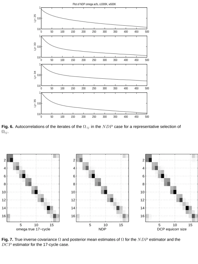
Figures 5 and Figure 6 are the autocorrelation plots for theDCP andN DP models for a representative selection of Ωij. The figures show that the autocorrelations of the iterates of the Ωij decay rapidly to zero for theDCP model, but are far more dependent in theN DP model. This difference in dependence is due to the greater efficiency of the sampling scheme in the decomposable case. Grey scale plots of the true inverse covariance Ω and posterior mean estimates of Ω for theN DP estimator and the DCP estimator for the 17-cycle case indicated thatN DP andDCP performed similarly in the simulations. For brevity only the nondecomposable 17-cycle is presented as it represents a case of high non-decomposability. Figure 7 shows that even in this case, the grey scales are very similar.
0 50 100 150 200 250 300 350 400 450 500 −0.5
0 0.5
i,j= 25
Plot of DCP omega acfs, s50K, w50K
0 50 100 150 200 250 300 350 400 450 500 −0.5 0 0.5 i,j= 33 0 50 100 150 200 250 300 350 400 450 500 −0.5 0 0.5 i,j= 34 0 50 100 150 200 250 300 350 400 450 500 −0.5 0 0.5 i,j= 35
Fig. 5. Autocorrelations of the iterates of theΩijin theDCP case for a representative selection of Ωij.
0 50 100 150 200 250 300 350 400 450 500 0.6
0.8 1
i,j= 25
Plot of NDP omega acfs, s1000K, w500K
0 50 100 150 200 250 300 350 400 450 500 0.6 0.8 1 i,j= 33 0 50 100 150 200 250 300 350 400 450 500 0.6 0.8 1 i,j= 34 0 50 100 150 200 250 300 350 400 450 500 0.6 0.8 1 i,j= 35
Fig. 6. Autocorrelations of the iterates of theΩijin theNDP case for a representative selection of
Ωij.
omega true 17−cycle
5 10 15 2 4 6 8 10 12 14 16 NDP 5 10 15 2 4 6 8 10 12 14 16 DCP equicorr size 5 10 15 2 4 6 8 10 12 14 16
Fig. 7. True inverse covarianceΩand posterior mean estimates ofΩfor theNDPestimator and the DCP estimator for the 17-cycle case.
A. Proofs of results Proof of Theorem 1
Roverato (2000) shows that if Σ∼HIW(g, δ,Φ) and Ω = Σ−1 then
p(Ω|g, δ,Φ)∝ |Ω|(δ−2)/2etr −1 2ΩΦ (22)
The result then follows from (7) since
p(Ω|y, g, δ,Φ)∝p(y|Ω)p(Ω|g, δ,Φ) ∝ |Ω|(n−1)/2etr −1 2ΩSy |Ω|(δ−2)/2etr −1 2ΩΦ =|Ω|(n+δ−3)/2etr −1 2Ω (Sy+ Φ) .
Note that the conjugate prior result for Ω does not require the graphgto be decomposable.
Proof of Theorem 2 First
p(Y|δ,Φ, g) = p(Y|Σ, δ,Φ, g)p(Σ|δ,Φ, g)
p(Σ|Y, δ,Φ, g) . The result then follows from (2), (3), (7) and Theorem 1.
Proof of Theorem 3
From Equation (5.23), Lemma 5.5 of Lauritzen (1996)
Ω = k i=1 (ΣCiCi)−1 V − k i=2 (ΣSiSi)−1 V and hence E(Ω|Y, δ,Φ, g) = k i=1 E (ΣCiCi)−1|Y, δ,Φ, g V − k i=2 E (ΣSiSi)−1|Y, δ,Φ, g V .
Now Σ|Y, δ,Φ, g∼HIW (δ,Φ∗, g∗), so from Dawid and Lauritzen (1993), ifAis a complete set in g then (ΣAA)−1|Y, δ,Φ, g ∼ Wishart (δ∗+|A| −1,Φ∗AA). The result then follows from the properties of the Wishart distribution.
Proof of Lemma 5
(a) For a nondecomposable graph to have 4 edges it must contain exactly one chordless 4-cycle and no other edges. There are p4possible choices for the 4 vertices, and for each choice of 4 vertices there are 3 different chordless 4-cycles.
(b) For a graph to be nondecomposable withp2−2 edges it must contain exactly one 4 cycle and all other edges must be present. Then apply the proof of the above. (c) We can partition the nondecomposable graphs with 5 edges into 2 sets: (a) those
with a chordless 5-cycle and no other edges, and (b) those with a chordless 4-cycle and an extra edge. For case (a) there are p5choices for the 5 vertices and for each choice there are (5−1)!/2 = 12 different chordless 5-cycles. For case (b) there are
p
4
×3 choices for the chordless 4-cycle, and for each choice of chordless 4-cycle there are (p2−6) choices for the extra vertex pair constituting the edge.
B. HIW results for Bayesian analysis using MCMC
The following results derive an expression for (15) that can be evaluated efficiently. The first theorem gives some necessary graph theory.
Letg= (V, E) be a decomposable graph with edge indicators{eij, i < j≤p}. Assume the edge indicatoreij = 1 forg, and that the graphg= (V, E) is decomposable and has edge setE as defined by indicators{eij = 0, e−ij}.
Theorem 6. Suppose that g and g are the decomposable graphs defined above. Suppose that C1, . . . , Ck are the cliques of g ordered to form a perfect sequence and S2, . . . , Sk are
the corresponding separators. Then
(a) The edge(i, j)is contained in a single clique ofg. (b) If(i, j)∈Cq then either i /∈Sq or j /∈Sq.
(c) Ifj /∈Sq andCq1 =Cq\{j} andCq2 =Cq\{i} thenC1,. . .,Cq−1,Cq1,Cq2,Cq+1,. . .,
Ck is a perfect sequence of complete sets in g and has separatorsS2,. . .,Sq−1,Sq1 =Sq,
Sq2 =Cq\{i, j},Sq+1,. . .,Sk.
(d) The sequenceC1,. . .,Cq−1,Cq1,Cq2,Cq+1,. . .,Ck contains all the cliques ofg.
Proof. Part (a) is Theorem 1 of Frydenberg and Lauritzen (1989) . Parts (b) and (c) follow from part (a) and Lemma 2.20 of Lauritzen (1996).
To show part (d), suppose thatC∗ is a clique of g. Then C∗ is complete ing, soC∗⊂Cl for somel ∈ {1, . . . , k}. IfC∗ ⊂Cq then part (b) implies that eitheri /∈Sq or j /∈Sq. So eitherC∗ ⊂Cq1 or C∗⊂Cq2. HenceC∗ is contained in at least one ofC1,. . ., Cq−1, Cq1,
Cq2,Cq+1,. . .,Ck. Part (c) shows thatC1,. . .,Cq−1,Cq1,Cq2,Cq+1,. . .,Ck are complete sets ing and the result follows.
The next lemma uses (4) and Theorem 6 to simplify (15).
Lemma 7. Suppose thatg andg are the decomposable graphs defined above. Then, using the notation of (12), and Theorem 6
h(g, δ,Φ) h(g, δ,Φ) h(g, δ∗,Φ∗) h(g, δ∗,Φ∗) = ΦDD|Sq2 δ+|Sq2|+1 2 Φ∗ii|Sq 2 δ∗+|Sq2| 2 Φ∗jj|Sq 2 δ∗+|Sq2| 2 Φii|Sq2 δ +|Sq2| 2 Φjj|Sq2 δ +|Sq2| 2 Φ∗DD|Sq 2 δ∗ +|Sq2|+1 2 × Γ δ+|Sq2| 2 Γ δ∗+|Sq 2|+1 2 Γ δ+|Sq2|+1 2 Γ δ∗+|Sq2| 2 , (23) whereD={i, j},ΦDD|Sq2 = ΦDD−ΦDSq2 ΦSq2Sq2 −1 ΦSq2D, andΦii|Sq2,Φjj|Sq2,Φ∗DD|Sq2, Φ∗ii|Sq 2 andΦ ∗
Proof. To obtain an expression forh(g, δ,Φ) we require the following technical lemma based on Lemma 2.13 of Lauritzen (1996).
Lemma 8. Let C1,. . .,Ck be a perfect sequence with separatorsS2,. . .,Sk. Assume that
Ct⊂Cp for somet=pand thatpis minimal with this property for fixed t. Then
(a) If p < t then St = Ct and C1, . . ., Ct−1, Ct+1, . . ., Ck is a perfect sequence with
separatorsS2,. . .,St−1,St+1,. . .,Sk
(b)If p > t then Sp =Ct and C1, . . ., Ct−1, Cp, Ct+1, . . ., Cp−1, Cp+1, Ck is a perfect sequence with separatorsS2,. . .,St−1,St,St+1,. . .,Sp−1,Sp+1,Sk
Proof of Lemma 8. See Lemma 2.13 of Lauritzen and its proof.
From Lemma 8, a perfect sequence of complete setsC1,. . .,Ck containing the cliques ofg
can be thinned by removing complete sets that are not cliques and reordering the sequence. From Lemma 8, the right-hand side of (4) is invariant to this thinning process. Successive application of the thinning process gives a perfect sequence consisting of the cliques ofg. From (4), Theorem 6 and Lemma 8
h(g, δ,Φ) = i=1,...q−1,q1,q2,q+1,...,k ΦCiCi 2 δ+|Ci|−1 2 Γ|Ci| δ+|Ci|−1 2 −1 i=2,...q−1,q1,q2,q+1,...,k ΦSiSi 2 δ+|Si|−1 2 Γ|Si| δ+|Si|−1 2 −1 . (24)
Now consider the ratioh(g, δ,Φ)/h(g, δ,Φ). Simplifying the expressions from (4) and (24) gives h(g, δ,Φ) h(g, δ,Φ) = ΦCqCq δ +|Sq2|+1 2 ΦSqSq δ +|Sq2|−1 2 Γ δ+|Sq2| 2 ΦCq1Cq1 δ +|Sq2| 2 ΦCq2Cq2 δ +|Sq2| 2 Γ δ+|Sq2|+1 2 2√π . (25) Substituting ΦCqCq=ΦDD|Sq 2 ΦSq2 ΦCq 1Cq1=Φii|Sq2ΦSq2 ΦCq 2Cq2=Φii|Sq2ΦSq2 into (25) gives h(g, δ,Φ) h(g, δ,Φ)= ΦDD|Sq2 δ +|Sq2|+1 2 Γ δ+|Sq2| 2 Φii|Sq2 δ +|Sq2| 2 Φjj|Sq2 δ +|Sq2| 2 Γ δ+|Sq2|+1 2 2√π .
A similar expression can be derived for the ratio h(g, δ∗,Φ∗)/h(g, δ∗,Φ∗) and the result follows.
The following lemma gives an efficient method for evaluating the terms in (23) using Cholesky decompositions.
Lemma 9. Using the notation of Theorem 6 and Lemma 7, suppose that the matrixACqCq > 0 is partitioned as ACqCq = ASq2Sq2 ASq2D ADSq2 ADD
and has Cholesky decomposition ACqCq =LL where
L= LSq2Sq2 0 LDSq2 LDD and LDD= lαα 0 lβα lββ . Then (a)ADD|Sq2 =LDD(LDD) (b)ADD|Sq2 = (lαα)2(lββ)2 (c)Aαα|Sq2 = (lαα)2 (d)Aββ|Sq2 = (lβα)2+ (lββ)2
Proof. The proof is straightforward and is omitted.
Equation (15) and parts (b)—(d) of Lemma 9give an efficient expression for the conditional distributions in Section 4. The main computational effort is in updating the Cholesky decompositions of the matrices ΦCqCq and Φ∗CqCq whenever an edge is added or deleted. From Lemma 9, these Cholesky decomposition must be done with the entries for theith andjth vertices in the lower right corner. Note that efficient Cholesky updating routines using Givens rotations are available in Matlab and Fortran. Note also that the dimensions of ΦCqCqand Φ∗CqCq depend on the cliques sizes and may be much smaller thanp. Thus our method has the local computational properties described in Giudici and Green (1999) and will have similar computational cost to their method per iteration of the Gibbs sampler.
Acknowledgement
The research of Robert Kohn and Helen Armstrong was partially supported by an Australian Research Council Grant.
References
Atay-Kayis, A. and H. Massam (2005). A Monte Carlo method to compute the marginal likelihood in non decomposable graphical gaussian models. Biometrikain press.
Barnard, J., R. McCulloch, and X. Meng (2000). Modeling covariance matrices in terms of standard deviations and correlations, with application to shrinkage.Statistica Sinica 10, 1281–1311.
Brooks, S., P. Giudici, and G. O. Roberts (2003). Efficient construction of reversible jump Markov chain Monte Carlo proposal distributions (with discussion). J. Royal Statistical Society B 65(1), 3–55.
Castelo, R. and N. Wormald (2001). Enumeration of p4-free chordal graphs. Journal of Graphs and Combinatorics (in press), or Universiteit Utrecht, Technical Report UU-CS-2001-12, June 2001.
Chiu, T., T. Leonard, and K. Tsui (1996). The matrix-logarithm covariance model.Journal of the American Statistical Association 81, 310–20.
Dawid, A. (1981). Some matrix-variate distribution theory: notational considerations and a Bayesian application. Biometrika 68(1), 265–274.
Dawid, A. P. and S. Lauritzen (1993). Hyper Markov laws in the statistical anlaysis of decomposable graphical models. The Annals of Statistics 21(3), 1272–1317.
Dellaportas, P. and J. Forster (1999). Markov chain Monte Carlo model determination for heirachical and graphical log-linear models. Biometrika 86(3), 615–633.
Dellaportas, P., P. Giudici, and G. Roberts (2004). Bayesian inference for non-decomposable graphical Gaussian models. Sankyha, Series A.
Dempster, A. (1972). Covariance selection. Biometrics 28, 157–175.
Dempster, A. P. (19 69 ). Elements of Continuous Multivariate Analysis. Reading, MA: Addison-Wesley.
Drton, M. and M. D. Perlman (2004). Model selection for Gaussian concentration graphs.
Biometrika 91(3), 591–602.
Efron, B. and C. Morris (1976). Multivariate Empirical Bayes estimation of covariance matrices. Annals of Statistics 4, 22–32.
Frydenberg, M. and S. Lauritzen (1989). Decomposition of maximum likelihood in mixed interaction models. Biometrika 76(3), 539–555.
Geiger, D. and D. Heckerman (2002). Parameter priors for directed acyclic graphical models and the characterization of several probability distributions. Annals of statistics 30(5), 1412–1440.
Giudici, P. (1996). Learning in graphical Gaussian models. In A. P. D. J. Berger, J. M. Bernardo and A. F. M. Smith (Eds.),Bayesian Statistics 5: Proceedings of the Fifth Valencia International Meeting, June 5-9, 1994, pp. 621–628. Oxford University Press. Giudici, P. and R. Castelo (2003). Improving Markov chain Monte Carlo model search for
data mining. Machine learning 50, 127–158.
Giudici, P. and P. J. Green (1999). Decomposable graphical Gaussian model determination.
Jones, B., C. Carvalho, A. Dobra, C. Hans, C. Carter, and M. West (2005). Experiments in stochastic computation for high-dimensional graphical models. Preprint.
Lauritzen, S. L. (1996). Graphical models. Oxford University Press.
Liechty, J. C., M. W. Liechty, and P. M¨uller (2004). Bayesian correlation estimation.
Biometrika 91(1), 1–14.
Mardia, K. V., J. T. Kent, and J. M. Bibby (19 79 ). Multivariate Analysis. London: Aca-demic Press.
Muirhead, R. (1982). Aspects of Multivariate Statistical Theory. Wiley.
Roverato, A. (2000). Cholesky decomposition of a hyper inverse Wishart matrix.
Biometrika 87, 99–112.
Roverato, A. (2002). Hyper inverse Wishart distribution for non-decomposable graphs and its application to Bayesian inference for Gaussian graphical models.Scandinavian Journal of Statistics 29, 391–411.
Smith, M. and R. Kohn (2002). Bayesian parsimonious covariance matrix estimation for longitudinal data. Journal of the American Satistical Association 87, 1141–1153. Wong, F., C. Carter, and R. Kohn (2003). Efficient estimation of covariance selection
models. Biometrika 90, 809–830.
Wormald, N. (1985). Counting labelled chordal graphs. Graphs and combinatorics 1, 193– 200.
Yang, R. and J. Berger (1994). Estimation of a covariance matrix using the reference prior.