Correction of electrode modelling errors in multi-frequency EIT imaging

(1)

This content has been downloaded from IOPscience. Please scroll down to see the full text.

Download details:

IP Address: 128.41.61.111

This content was downloaded on 16/08/2016 at 15:07

Please note that terms and conditions apply.

Correction of electrode modelling errors in multi-frequency EIT imaging

View the table of contents for this issue, or go to the journal homepage for more 2016 Physiol. Meas. 37 893

(2)

893

Physiological Measurement

Correction of electrode modelling errors in

multi-frequency EIT imaging

Markus Jehl and David Holder

University College London, London WC1E 6BT, UK E-mail: [email protected]

Received 30 November 2015, revised 14 January 2016 Accepted for publication 25 January 2016

Published 20 May 2016 Abstract

The differentiation of haemorrhagic from ischaemic stroke using electrical impedance tomography (EIT) requires measurements at multiple frequencies, since the general lack of healthy measurements on the same patient excludes time-difference imaging methods. It has previously been shown that the inaccurate modelling of electrodes constitutes one of the largest sources of image artefacts in non-linear multi-frequency EIT applications. To address this issue, we augmented the conductivity Jacobian matrix with a Jacobian matrix with respect to electrode movement. Using this new algorithm, simulated ischaemic and haemorrhagic strokes in a realistic head model were reconstructed for varying degrees of electrode position errors. The simultaneous recovery of conductivity spectra and electrode positions removed most artefacts caused by inaccurately modelled electrodes. Reconstructions were stable for electrode position errors of up to 1.5 mm standard deviation along both surface dimensions. We conclude that this method can be used for electrode model correction in multi-frequency EIT.

Keywords: electrical impedance tomography, stroke type detection, multi-frequency image reconstruction, electrode model correction (Some figures may appear in colour only in the online journal)

1. Introduction

1.1. Background

Multifrequency electrical impedance tomography (MFEIT) is a method for imaging biologi-cal tissues with frequency-dependent conductivity. While time-difference (TD) EIT is used M Jehl and D Holder

Correction of electrode modelling errors in multi-frequency EIT imaging

Printed in the UK

893

PMEAE3

Institute of Physics and Engineering in Medicine

Original content from this work may be used under the terms of the Creative Commons Attribution 3.0 licence. Any further distribution of this work must maintain attribution to the author(s) and the title of the work, journal citation and DOI. 0967-3334/16/060893+11$33.00 © 2016 Institute of Physics and Engineering in Medicine Printed in the UK

(3)

to image conductivity changes between a baseline voltage measurement and a data measure-ment, MFEIT differentiates tissues based on their conductivity spectra at different modulation frequencies of the applied current. Therefore MFEIT does not require a baseline measurement and can be used as a diagnostic tool for multiple applications (Brown et al1995, Hampshire

et al1995, Malich et al2003), including stroke type differentiation (Holder 1992, Romsauerova

et al2006, Packham et al2012).

While cerebral haemorrhages require surgery, ischaemic strokes could be treated with a clot dissolving drug if diagnosed within 3 h of onset. The current diagnostic procedure is to take a computed tomography (CT) scan, and results in only 2.5–6% of the 80% of ischaemic strokes to be treated in time (Power 2004, Saver et al2013). While EIT cannot compete with CT in terms of image quality, the small size and low cost of an EIT system make it feasible to equip ambulances for early ischaemia diagnosis and thrombolytic treatment.

A novel non-linear method for performing MFEIT using spectral constraints was recently proposed by Malone et al (2014a), because the complicated geometry of the head excludes linear multi-frequency reconstruction algorithms, such as weighted frequency difference (Jun

et al2009). In the new MFEIT algorithm, the inverse problem is reformulated to express the conductivity at each frequency in terms of tissue volume fractions and known tissue conduc-tivity spectra. This separation of variables makes it possible to use measurements at different frequencies simultaneously, since the tissue fractions are frequency independent. An analysis of the influence of modelling errors on images reconstructed with this method has shown that inaccurately modelled electrode positions strongly affect the image quality, whereas wrongly modelled contact impedances were negligible and spectral errors were tolerable as long as tissue spectra did not overlap (Malone et al2014b).

Methods for correction of electrode modelling inaccuracies are recently gaining interest in the EIT community (Soleimani et al2006, Dardéet al2012), and have already been applied to a realistic three dimensional head model for simultaneous TD recovery of conductivity changes and electrode movement (Jehl et al 2015b). In this paper, the first application of simultaneous MFEIT image reconstruction and electrode model correction is demonstrated on a realistic 3D head model with skull and scalp. The implementation is discussed and the performance is evaluated for different levels of electrode position errors.

1.2. Purpose

The purpose of this study is to evaluate the performance of simultaneous recovery of electrode positions and conductivity spectrum changes. Specifically, the following two questions will be addressed:

(i) Does the simultaneous recovery of conductivity changes and electrode modelling errors remove image artefacts caused by inaccurately modelled electrode positions?

(ii) At which magnitude of electrode position errors does the proposed algorithm begin to fail?

To answer these questions, multi-frequency boundary voltages were simulated on a fine 5 million element head mesh with different levels of electrode position errors. Reconstructions were made with and without the proposed addition of electrode modelling corrections and the resulting images were compared. It was found that the proposed algorithm could stably recover simulated strokes in the presence of electrode modelling errors of up to 1.5 mm stand-ard deviation.

(4)

2. Methods

2.1. Tissue fraction reconstruction with electrode position correction

The general structure of the used multi-frequency reconstruction algorithm was identical to the one published by Malone et al (2014a). To be able to use conductivity measurements at different frequencies ωi,i= …1, ,W simultaneously in a single image reconstruction, the conductivity spectrum of one element in the mesh was described as a linear combination of the known spectra of present tissues t jj, = …1, ,T. Instead of reconstructing conductivities directly, the prior knowledge of the conductivity spectrum εij of all tissues was therefore used to assign fractions fnj of these tissues to all finite elements n= …1, ,N, such that

( )

∑

σ ω = ⋅ = ε f , n i j T nj ij 1 (1) where 0⩽ ⩽f_nj 1, ∑T_j₌ f =1 nj

1 and fj∈R1×N=[f1j,…,fNj]. The modified Jacobian matrix at each frequency was obtained from the non-linear EIT forward map A using the chain rule

( )σ _{( )} σ σ σ σ ∂ ∂ = ∂ ∂ ∂ ∂ = ∂ ∂ ε = ⋅ε = ∈R × f f A A A _J _J , i j i i j i ij i ij ij R N (2) where r= …1, ,R are the lines in the protocol, i.e. the combinations of different current injec-tion and voltage measurement electrode pairs d and m. The Jacobian matrix J( )σi relating voltage changes to changes in conductivity σi at each frequency ωi, was computed using the adjoint fields method (derived e.g. in the appendix of Polydorides and Lionheart (2002)), giving one entry for element n as

∫

= − ∇u ⋅ ∇u V Jrn d , n d m (3) where ud∈H1_{( )}Ω_{is the electric potential emerging when the drive current}_Id_{is applied to} the electrodes and um∈H1_{( )}Ω_{the electric potential when a unit current is applied to the two} measurement electrodes.

In order to correct for wrongly modelled electrode positions, this _‘traditional_’ Jacobian matrix was augmented by an electrode boundary Jacobian _EBJ∈_RR E× _{, relating electrode} boundary changes (in our case electrode movement) to voltage changes. Given a continuous vector field v on the boundary of electrode e= …1, ,E, one entry of the EBJ can be computed similarly to the conductivity Jacobian (Dard_éet al2012, Jehl et al2015b)

( )( )( )

∫

= − ⋅ − − ∂ v n∂ u u z U U s EBJre 1 d , e E E e d d e m m e (4) where ze is the contact impedance, U_ed and U_em the drive and measurement electrode potentials and n∂E the outward normal of the electrode boundary, tangential to the head surface. The vector field v describes the studied change in the electrode boundary, e.g. to compute the EBJ

with respect to movement along one direction, the vector field was chosen to point homo-geneously in this direction. The Jacobian matrices were combined ϒi=[Ji1,…,J EBJiT, i]

and the unknown electrode position errors p were appended to the vector of the tissue frac-tions to be recovered _x₌[_{f p}_, ]_{, where}_f _f_, _,_f

T 1

[ ]

= … and p consisted of two variables per electrode that described electrode movements along both surface directions xs and ys,

[ ]

= …

p p p p p1_x_s, 1_y, _x2, _y2,

(5)

( )

∑

(ϒ ϒ) ( ( )ω ( ))ω τ ( ) Φ = − − − + Ψ = ⎡ ⎣ ⎢ ⎤ ⎦ ⎥ x 1 x v v x 2 _i , W i i 2 1 1 2 (5) with v( )ωi being the boundary voltages measured at frequency ωi and the regularisation term

( ) Σ Σ

Ψ_x =_x _{D D} _x_.

x x

(6) The regularisation matrix D comprised one Laplacian matrix per recovered tissue and one identity matrix for the electrode movement variables. All components were scaled accord-ing to the expected standard deviation of the correspondaccord-ing variable changes stdf =0.01 and

= stdp 1 mm Σ = = ⋅ ⋅ ⋅ − − − ⎡ ⎣ ⎢ ⎢ ⎢ ⎤ ⎦ ⎥ ⎥ ⎥ ⎡ ⎣ ⎢ ⎢ ⎢ ⎢ ⎢ ⎤ ⎦ ⎥ ⎥ ⎥ ⎥ ⎥ D L L I I I I 0 0 0 0 0 0 0 0 0 0 0 0 ; std 0 0 0 0 0 0 0 0 std 0 0 0 0 std . x f f p 1 1 1 (7)

The minimisation of the objective function (5) was performed by alternating steps of gradi-ent projection) and damped Gauss–Newton algorithms. The gradient projection (Nocedal and Wright 1999) step was used to quickly move to the neighbourhood of the minimum, while considering the constraints on the fractions. This was done by computing the step sizes along the gradient, at which one of the fraction values reaches a constraint, i.e. 0 or 1. The change of the objective function value along each of the resulting intervals was approximated quadrati-cally using Taylor series. Once one Taylor approximation found a minimum on an interval, this so-called Cauchy point xc was chosen, otherwise the gradient projection algorithm con-tinued on the next interval until a minimum was found.

The subsequent Gauss–Newton step was only applied to the components that did not reach a constraint during the gradient projection. The search direction was calculated by solving

( )x ⋅ = −∇d Φ( )x

H c c

(8) using a generalised minimal residual algorithm in order to avoid the explicit calculation of the Hessian matrix H, which is the second derivative of Φ( )x (which was approximated by disre-garding the second order derivative of the residual error). The step width along direction d was determined using the Brent line-search method (Brent 1973) and the resulting minimum xg was projected back to the fraction constraints. The point, xc or xg, that gave a smaller function value was chosen for the next iteration.

The reconstruction of the fractions was constrained to the closed interval [0, 1] and the constraint ∑T_j₌ f =1

nj

1 was enforced by substituting f1 = − ∑1 Tj=2fj. After two iterations of gradient projection and Gauss–Newton, the electrode positions had normally converged and were subsequently kept fixed for the remaining iterations. The number of iterations of this reconstruction algorithm was fixed to 10 for all image reconstructions. To avoid the inverse crime (Lionheart 2004) and speed up image reconstruction, all reconstruction were made on a coarse 180 thousand element mesh on which the skull and scalp were kept fixed and it was assumed the inside of the skull was occupied by either the brain or the stroke with the ini-tial guess being the healthy brain. The regularisation parameter of τ= ×₈ ₁₀−10_{was chosen} empirically and was the same for all reconstructed images. After each iteration of gradient projection and Gauss–Newton minimisation, the regularisation parameter was halved in the case of ischaemias, and given that the spectral contrast was lower, divided by three for haem-orrhages (Viklands and Gulliksson 2001, Malone et al2014b).

(6)

2.2. Data simulation

The simulation parameters in this study were identical to the ones used in the preliminary feasibility study (Malone et al2014b). Boundary voltages were computed on a fine 5 million element mesh, which was created from a CT scan of a human head and included three homo-geneous tissues: brain, skull and scalp. Computation of the boundary voltages was done with Peits (Jehl et al2015a) on all 16 processors of a workstation with two 2.4 GHz Intel Xeon CPUs with eight cores and 20 MB cache each. It took less than 2 min to compute the required 31 forward solutions for each frequency. 32 electrodes of diameter 10 mm were placed on the surface of the model in the same positions used to acquire EEG measurements (Tidswell et al

2001). The electrodes were modelled using the complete electrode model (CEM) (Somersalo

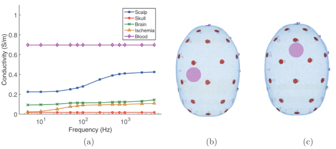
et al1992), and the contact impedance was set to 1kΩ ⋅| |E for all electrodes, where | |E was the electrode area. The amplitude of the current was set to 140 μA and twelve frequencies between 5 Hz and 5 kHz were used (figure 1(a)). 31 linearly independent current injection pairs were created by finding the maximum spanning tree of the electrode positions, thereby maximising the distance between injecting electrodes. Voltage measurements were made for each injection on all adjacent pairs not involved in delivering current. The total number of measurements acquired for each frequency was 869.

Strokes were simulated by changing the conductivities of all elements within a 1.5 cm radius of the stroke location. Simulated locations were set in a posterior (figure 1(c)) or lateral position in the head (figure 1(b)), and stroke conductivities were set to the spectral values of ischaemic tissue (figure 1(a)) or to the conductivity of blood, 0.697 S m−1_{, for haemorrhage} (Horesh 2006). Both proportional and additive noise was added to all simulated voltages:

( ( ))ς ( )ς

= + +

vwith noise vno noise1 rand p rand a ,

(9) where rand( )ς indicates a random number drawn from a Gaussian distribution with zero mean and standard deviation ς. The standard deviation of the proportional noise was ςp=0.02% and the standard deviation of the additive noise was ςa=5 V µ , which correspond to human

measurements (Goren et al2015).

Electrode positions can currently be measured to around 1 mm precision using photogram-metry (Qian and Sheng 2011). Other technologies, such as the commercial MicroScribe, laser 3D scanners, or electrode helmets, can achieve an even higher precision in electrode Figure 1. Model: (a) conductivity spectra of the simulated tissues, (b) simulated lateral and (c) posterior stroke position. These simulation parameters were already used in Malone et al (2014b). CC BY Frequency (Hz) 101 102 103 Conductivity (S/m) 0 0.2 0.4 0.6 0.8 1 Scalp_Skull Brain Ischemia Blood (a) (b) (c)

(7)

localisation. Simulated electrode position errors were therefore created by drawing two random numbers for each electrode from Gaussian distributions with zero mean and standard deviations 0.5 mm, 1 mm, 1.5 mm and 2 mm. According to these drawn random numbers, the electrodes were then moved along a two dimensional surface coordinate system Jehl et al

(2015b). Consequently, the overall electrode position errors were the combined errors of the displacement along the two surface dimensions, and deviations of up to three times the stand-ard deviation of the error were expected in the majority of cases.

Previous methods for computing the electrode movement Jacobian include the compu-tationally intensive differential approximations by moving nodes in the mesh (Soleimani

et al2006), which are limited to relatively coarse meshes, direct methods based on the mesh geometry (Gómez-Laberge and Adler 2008) and the approximation error approach (Nissinen

et al2011). However, the analytical formulation of the Fréchet derivative with respect to the electrode boundary presented by Dardéet al (2012) is the most flexible approach, since it can be used for different electrode characteristics independent of mesh refinement and can be implemented in a very fast and memory efficient way (Jehl et al2015b). Another advantage of this implementation is the possibility to move electrodes without altering the mesh geometry, by changing the assignment of the surface facets to the electrodes instead. This allows for larger movement of electrodes, while maintaining a good mesh quality and refinement. 2.3. Image quantification

The quality of an image was objectively quantified in terms of the ability to distinguish the stroke from the brain. This was done by assessing the fraction f_s corresponding to the tissue that made up the anomaly. First, the images reconstructed on the 180 thousand element mesh were averaged onto cubic voxels with 0.5 cm sides. The volume P corresponding to the reconstructed perturbation was identified as the largest connected cluster of voxels with values larger than 50% of the maximum of the image (Malone et al2014a, Jehl et al2015b). Three measures of image errors were defined:

(i) Location error: ratio between the distance ∥(x y zP, ,P P)∥ of the centre of mass of the

recon-structed perturbation P from the actual position, and the average dimension of the head

(d d d) mean x, ,y z ∥( )∥ ( ) x y z d d d , , mean , , . P P P x y z (10) (ii) Shape error: ratio of the difference between the dimensions of the simulated (s s sx, ,y z) and

reconstructed perturbation (r r rx, ,y z), and the dimensions of the simulated perturbation

∥( )∥ ∥( )∥ − − − r s r s r s s s s , , , , . x x y y z z x y z (11) (iii) Image noise: inverse of the contrast-to-noise ratio between the perturbation P and the

background B ( ) ¯ −¯ f f f std , s B s P s B (12) where f¯_sP and f¯_sB are the mean intensities of the perturbation and background and std the

(8)

3. Results

3.1. Multi-frequency tissue fraction reconstructions

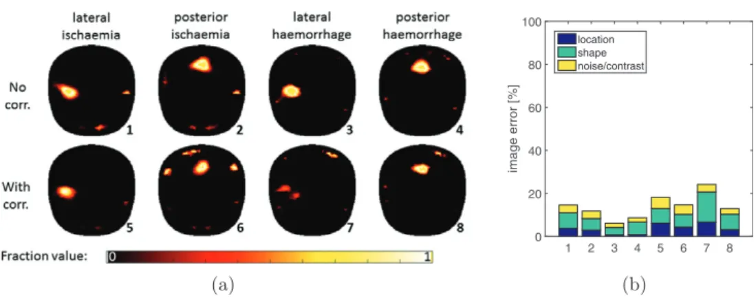
When electrode positions were modelled accurately in the reconstruction algorithm, image reconstructions with electrode modelling correction were slightly worse than without correc-tion (figure 2(a)). The average image error of reconstructions without electrode correction was 10% and with correction 17%; particularly the reconstruction of the lateral haemorrhage was not good (24%). The reason for the decreased image quality was the larger number of variables to recover, which slightly increased the ill-posedness of the inverse problem. Consequently, conductivity changes were sometimes explained by electrode movements, if this reduced the value of the objective function.

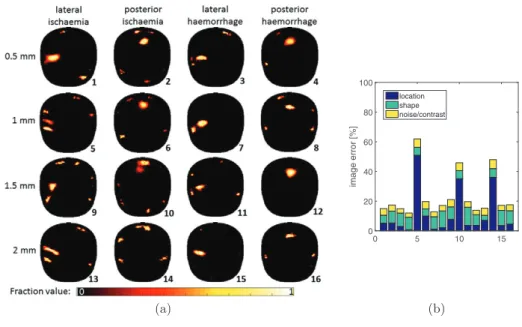
With the traditional fraction reconstruction MFEIT algorithm, already 0.5 mm of electrode position modelling errors made stroke detection impossible (figure 3(a)). The average image error of the reconstructions without electrode modelling correction was 55% (figure 3(b)).

Simultaneous recovery of stroke tissue fractions and electrode positions significantly improved image quality in the presence of electrode modelling errors (figure 4(a)). The aver-age imaver-age error of the reconstructed imaver-ages with correction was 23% (figure 4(b)), excluding the three outliers (numbers 5, 10 and 14) only 16%. Remarkably, all three bad reconstructions occurred for ischaemic strokes, suggesting that local conductivity spectrum changes caused by ischaemia were more difficult to separate from electrode position errors than for haemor-rhage. Such image errors are the result of the combination of errors added to the simulated voltages and the combined uncertainty on all electrode positions, and are consequently diffi-cult to characterise. The shape error of the reconstruction of a lateral ischaemia with electrode movement of 2 mm (number 13) is misleadingly small, because the recovered perturbation was a diagonal disc with very similar x–y–z dimensions than the simulated stroke.

3.2. Electrode placement correction

The 2-norm of the difference between recovered and simulated electrode position mismatch for both surface dimensions (dx and dy) was computed as

(

∑_idx_i2+dy_i2 1/2

)

, for electrodes

i. While the electrode position correction was more accurate for ischaemic strokes when electrodes were correctly modelled, for position mismatch of 1 mm standard deviation the Figure 2. (a) Multi-frequency fraction reconstructions of strokes without and with electrode modelling correction when electrodes were modelled accurately and (b) the corresponding image error measures.

(a) 1 2 3 4 5 6 7 8 image error [% ] 0 20 40 60 80 100 location shape noise/contrast (b)

(9)

correction was better in the presence of haemorrhages (table 1). The accuracy of the electrode position recovery tended to correlate with the quality of the reconstructed image (figures 2(a) and 4(a)). This is intuitive and was already observed for time-difference electrode movement corrections (Jehl et al2015b).

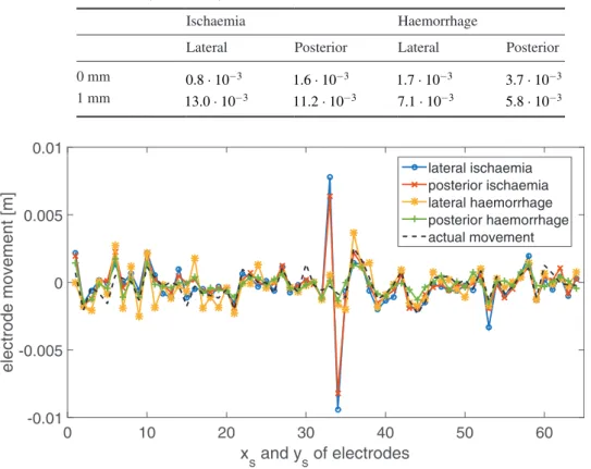
The reason for the worse 2-norm of ischaemic electrode position correction of 1 mm errors, was electrode 17 (entries 33 and 34 on x-axis of figure 5). Interestingly, after one iteration of the proposed algorithm, the electrode position recovery of this electrode was still accurate. Only in the second iteration, the electrode was moved several millimetres in both surface dimensions. Since electrode 17 was located laterally, 5.4 cm from the centre of the lateral ischaemia, this affected the reconstruction of the lateral ischaemia more than the reconstruc-tion of the posterior ischaemia (figure 4(a)).

Figure 3. (a) Multi-frequency fraction reconstructions of strokes without electrode modelling correction for two different levels of electrode position errors and (b) the corresponding image error measures.

(a) 1 2 3 4 5 6 7 8 image error [%] 0 20 40 60 80 100 location shape noise/contrast (b)

Figure 4. (a) Multi-frequency fraction reconstructions of strokes using electrode correction for four different levels of electrode position modelling errors and (b) the corresponding image error measures.

(a) 0 5 10 15 image error [%] 0 20 40 60 80 100 location shape noise/contrast (b)

(10)

4. Discussion

The simultaneous recovery of stroke tissue fractions and electrode positions significantly improved image quality in the presence of electrode modelling errors and had only small negative effects on the image quality when electrode were modelled accurately. For move-ments between 0.5 mm and 2 mm standard deviation along both surface dimensions, the average image error was 23% compared to 55% without electrode correction. While recon-structions of haemorrhagic strokes were even successful in the presence of 2 mm of electrode errors, ischaemia detection was less reliable from 1 mm onwards. The lower reliability could be caused by a worse differentiability of ischaemic changes to electrode movements, but this could so far not be confirmed.

Ideally, several reconstructions would have been made for each electrode movement level in order to characterise the effect of electrode modelling errors over a number of samples. However, the computational expense of multiple repetitions was prohibitive, since reconstruc-tion of a single image took around 6 h. For the same reason, only two stroke posireconstruc-tions were

Table 1. 2-norm of the difference in simulated and recovered electrode position errors when electrodes were accurately modelled in the reconstruction algorithm (first row) and when there was a position mismatch of 1 mm standard deviation along both surface dimensions (second row).

Ischaemia Haemorrhage

Lateral Posterior Lateral Posterior 0 mm _{0.8 10}_⋅ −3 _{1.6 10}_⋅ −3 _{1.7 10}_⋅ −3 _{3.7 10}_⋅ −3

1 mm _{13.0 10}_⋅ −3 _{11.2 10}_⋅ −3 _{7.1 10}_⋅ −3 _{5.8 10}_⋅ −3

Figure 5. Recovery of electrode position modelling errors for different stroke types and positions, when electrodes were simulated with standard deviation of 1 mm positional errors (black dashed line). Along the x-axis are the movement components along both surface dimensions for each electrode, i.e. 1&2 are xs and ys of electrode 1, 3&4 for electrode 2 and so on.

x_s and y_s of electrodes 0 10 20 30 40 50 60 electrode movement [m] -0.01 -0.005 0 0.005 0.01 lateral ischaemia posterior ischaemia lateral haemorrhage posterior haemorrhage actual movement

(11)

studied. Nonetheless, the produced images clearly illustrate the advantage of simultaneous tissue fraction and electrode position recovery in the presence of electrode modelling errors.

Many methods for computing the Jacobian matrix with respect to electrode movement could have been used on the multi-frequency data. The presented method for correction of inaccurate electrode modelling had the advantage over previous approaches, that the mesh geometry did not have to be altered. This allowed for the iterative recovery of movements of several millimetres on fine meshes, which is not possible with traditional differential approaches for electrode movement recovery (Soleimani et al2006). Furthermore, the imple-mentation based on the Fréchet derivative (Dardéet al2012) used here has been shown to be fast and memory efficient (Jehl et al2015b).

5. Conclusion

Simultaneous iterative electrode position correction with the fraction reconstruction method using spectral constraints was applied to a numerical head phantom with realistic conductivi-ties. Realistic noise was added to the simulated voltages to investigate the robustness of the proposed method. The results show that

(i) the simultaneous recovery of tissue volume fractions and electrode position errors removed most image artefacts caused by inaccurately modelled electrodes.

(ii) while haemorrhagic strokes could be reconstructed with electrode position errors up to 2 mm standard deviation in both surface dimensions, the reconstruction of ischaemic strokes was less reliable from electrode movements of 1 mm onwards.

Further work is required to understand why ischaemic stroke reconstructions were less reliable with the proposed method, and to correct for it. Additionally, it has so far not been studied how stable non-linear multi-frequency reconstruction methods are in the presence of geometric modelling errors, such as skull shape. We plan to validate the presented results in tank experiments with 3D printed head shaped tanks and skull (Jehl et al2015b) and recom-mend the presented algorithm for any planned human studies.

References

Brent R 1973 Algorithms for Minimization Without Derivatives (Englewood Cliffs, NJ: Prentice-Hall) Brown B, Leathard A, Lu L, Wang W and Hampshire A 1995 Measured and expected Cole parameters

from electrical impedance tomographic spectroscopy images of the human thorax Physiol. Meas.

16 57–67

Dardé J, Hakula H, Hyvönen N and Staboulis S 2012 Fine-tuning electrode information in electrical impedance tomography Inverse Problems Imaging6 399–421

Gómez-Laberge C and Adler A 2008 Direct EIT Jacobian calculations for conductivity change and electrode movement Physiol. Meas.29 89–99

Goren N, Avery J and Holder D 2015 Feasibility study for monitoring stroke and TBI patients Proc. of the 16th Int. Conf. on Biomedical Applications of Electrical Impedance Tomography ed J Sol_à

et al p 71

Hampshire A, Smallwood R, Brown B and Primhak R 1995 Multifrequency and parametric EIT images of neonatal lungs Physiol. Meas.16 175_–89

Holder D 1992 Detection of cerebral ischaemia in the anaesthetised rat by impedance measurement with scalp electrodes: implications for non-invasive imaging of stroke by electrical impedance tomography Clin. Phys. Physiol. Meas.13 63

Horesh L 2006 Some novel approaches in modelling and image reconstruction for multi frequency electrical impedance tomography of the human brain PhD Thesis University College London

(12)

Jehl M, Dedner A, Betcke T, Aristovich K, Kl_öfkorn R and Holder D 2015a A fast parallel solver for the forward problem in electrical impedance tomography IEEE Trans. Biomed. Eng.62 126_–37 Jehl M, Avery J, Malone E, Holder D and Betcke T 2015b Correcting electrode modelling errors in EIT

on realistic 3D head models Physiol. Meas.36 2423_–42

Jun S, Kuen J, Lee J, Woo E, Holder D and Seo J 2009 Frequency-difference EIT (fdEIT) using weighted difference and equivalent homogeneous admittivity: validation by simulation and tank experiment

Physiol. Meas.30 1087_–99

Lionheart W 2004 EIT reconstruction algorithms: pitfalls, challenges and recent developments Physiol. Meas.25 125_–42

Malich A, B_öhm T, Facius M, Kleinteich I, Fleck M, Sauner D, Anderson R and Kaiser W 2003 Electrical impedance scanning as a new imaging modality in breast cancer detection a short review of clinical value on breast application, limitations and perspectives Nucl. Instrum. Methods Phys. Res.497 75_–81

Malone E, Sato Dos Santos G, Holder D and Arridge S 2014a Multifrequency electrical impedance tomography using spectral constraints IEEE Trans. Med. Imaging33 340_–50

Malone E, Jehl M, Arridge S, Betcke T and Holder D 2014b Stroke type differentiation using spectrally constrained multifrequency EIT: evaluation of feasibility in a realistic head model Physiol. Meas.

35 1051_–66

Nissinen A, Kolehmainen V and Kaipio J 2011 Compensation of modelling errors due to unknown domain boundary in electrical impedance tomography IEEE Trans. Med. Imaging30 231_–42 Nocedal J and Wright S 1999 Numerical Optimization(Series in Operations Research and Financial

Engineering) (New York: Springer)

Packham B, Koo H, Romsauerova A, Ahn S, McEwan A, Jun S and Holder D 2012 Comparison of frequency difference reconstruction algorithms for the detection of acute stroke using EIT in a realistic head-shaped tank Physiol. Meas.33 767_–86

Polydorides N and Lionheart W 2002 A matlab toolkit for three-dimensional electrical impedance tomography: a contribution to the electrical impedance and diffuse optical reconstruction software project Meas. Sci. Technol.13 1871_–83

Power M 2004 An update on thrombolysis for acute ischaemic stroke Adv. Clin. Neurosci. Rehabil.

4 36_–7

Qian S and Sheng Y 2011 A single camera photogrammetry system for multi-angle fast localization of EEG electrodes Ann. Biomed. Eng.39 2844_–56

Romsauerova A, McEwan A, Horesh L, Yerworth R, Bayford R and Holder D 2006 Multi-frequency electrical impedance tomography (EIT) of the adult human head: initial findings in brain tumours, arteriovenous malformations and chronic stroke, development of an analysis method and calibration

Physiol. Meas.27 147_–61 (PMID: 16636407)

Saver J, Fonarow G, Smith E, Reeves M, Grau-Sepulveda M, Pan W, Olson D, Hernandez A, Peterson E and Schwamm L 2013 Time to treatment with intravenous tissue plasminogen activator and outcome from acute ischemic stroke J. Am. Med. Assoc.309 2480_–8

Soleimani M, G_ómez-Laberge C and Adler A 2006 Imaging of conductivity changes and electrode movement in EIT Physiol. Meas.27 103_–13

Somersalo E, Cheney M and Isaacson D 1992 Existence and uniqueness for electrode models for electric current computed tomography SIAM J. Appl. Math.52 1023_–40

Tidswell T, Gibson A, Bayford R and Holder D 2001 Three-dimensional electrical impedance tomography of human brain activity NeuroImage13 283_–94

Viklands T and Gulliksson M 2001 Fast Solution of Discretized Optimization Problems (ISNM Int. Series of Numerical Mathematics vol 138) ed K Hoffmann et al (Basel: Birkh_äuser) pp 255_–64