Middlesex University Research Repository
An open access repository of
Middlesex University research
http://eprints.mdx.ac.uk
Yerworth, Rebecca J. and Bayford, Richard (2017) DICOM for EIT. In:
18th International Conference on Biomedical Applications of Electrical
Impedance Tomography, 21-24 June 2017, Hanover, New Hampshire,
USA.
http://dx.doi.org/10.5281/zenodo.557093
Published version (with publisher's formatting)
Available from Middlesex University’s Research Repository at
http://eprints.mdx.ac.uk/22326/
Copyright:
Middlesex University Research Repository makes the University’s research available electronically.
Copyright and moral rights to this thesis/research project are retained by the author and/or
other copyright owners. The work is supplied on the understanding that any use for
commercial gain is strictly forbidden. A copy may be downloaded for personal,
non-commercial, research or study without prior permission and without charge. Any use of
the thesis/research project for private study or research must be properly acknowledged with
reference to the work’s full bibliographic details.
This thesis/research project may not be reproduced in any format or medium, or extensive
quotations taken from it, or its content changed in any way, without first obtaining permission
in writing from the copyright holder(s).
If you believe that any material held in the repository infringes copyright law, please contact
the Repository Team at Middlesex University via the following email address:
Proceedings
!
of the
!
18
th
International Conference on
!
Biomedical Applications of
!
!
ELECTRICAL IMPEDANCE TOMOGRAPHY
!
!
Edited by Alistair Boyle, Ryan Halter, Ethan Murphy and Andy Adler
!
!
June 21-24, 2017
!
Thayer School of Engineering at Dartmouth
!
Each individual paper in this collection: c2017 by the indicated authors. Collected work: c2017 Alistair Boyle, Ryan Halter, Ethan Murphy, Andy Adler
This work is licensed under aCreative Commons Attribution 4.0 International License.
Funding for this conference was made possible (in part) by 1 R13 EB024401-01 from the National Institute of Biomedical Imaging and Bioengineering. The views expressed in written conference materials or publications and by speakers and moderators do not necessarily reflect the official policies of the Department of Health and Human Services; nor does mention of trade names, commercial practices, or organizations imply endorsement by the U.S. Government.
Printed in USA
DOI:10.5281/zenodo.557093
Thayer School of Engineering at Dartmouth 14 Engineering Drive
Hanover, New Hampshire USA
engineering.dartmouth.edu [email protected] (603) 646-2230
Table of Contents
Andrea BorsicAcceleration of EIT Image Reconstruction on Graphic Processing Units. . . 1
Henry F. J. TregidgoTowards Efficient Iterative Absolute EIT. . . 2
Mari Lehti-PolojärviRotational electrical impedance tomography with few electrodes. . . 3
Alistair BoyleSpatio-Temporal Regularization over Many Frames. . . 4
Nick PolydoridesImage reconstruction in Lorentz force Electrical Tomography. . . 5
Ethan K. MurphyFused-data Transrectal EIT incorporating Biopsy Electrodes. . . 6
Erfang MaConvergence of finite element approximation in electrical impedance tomography. . . 7
P. Robert KotiugaEIT in Multimodal Imaging for Avoiding Biopsies of False Positive Results in Mammography. . . 8
Sarah HamiltonDirect Absolute EIT Imaging on Experimental Data. . . 9
Bo GongEIT reconstruction regularized by Total Generalized Variation. . . 10
Michael G. CrabbThe sensitivity in time domain EIT. . . 11
Yeong-Long HsuEIT guided PEEP titration in ARDS: preliminary results of a prospective study. . . 12
Tzu-Jen KaoPulsatile Perfusion Imaging of Premature Neonates using SMS-EIT. . . 13
Geuk Young JangRegional Air Distributions in Porcine Lungs using High-performance Electrical Impedance Tomography System. . . 14
Songqiao LiuEffect of variable pressure support ventilation on ventilation distribution: preliminary results of a prospective study. . . 15
Étienne Fortin-PellerinMonitoring Ventilation and Perfusion in the liquid-ventilated lung. . . 16
Bartłomiej GrychtolFocusing EIT reconstructions using two electrode planes. . . 17
Sarah BuehlerDetection of the aorta in electrical impedance tomography images without the use of contrast agent. . . 18
Jakob OrschulikMeasurement Strategies for Heart Focused Dual Belt EIT. . . 19
Andrew TizzardRapid Generation of Subject-Specific Thorax Forward Models. . . 20
Chuong NgoCombination of Electrical Impedance Tomography and Forced Oscillation Technique: a new pulmonary diagnostics tool?. . . 21
Saaid H. ArshadCardio-Respiratory Gated Electrical Impedance Tomography for Monitoring Stroke-Volume. . . 22
Sonja M. WeizElectrical impedance tomography in on-chip integrated microtubular fluidic channels. . . 23
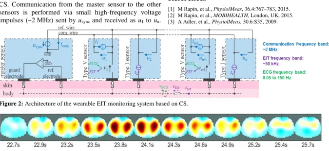
Michael RapinA wearable EIT system based on cooperative sensors. . . 24
Serena de GelidiTorso shape detection to improve lung monitoring. . . 25
Wrichik BasuImproved amplitude estimation of lung EIT signals in the presence of transients: Experimental validation using discrete phantoms. . . 26
Tobias MendenInfluence of multiplexers and cables on bio-impedance measurements. . . 27
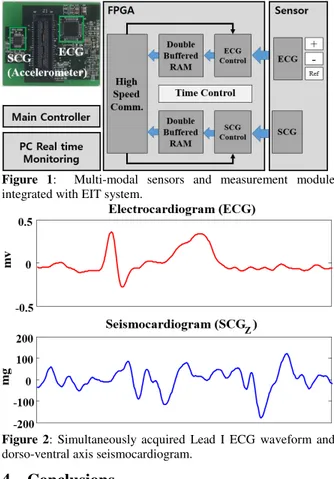
Hyuntae ChoiSeismocardiogram and EIT Images. . . 28 i
Keivan KaboutariAn Experimental Study for Magneto-Acousto Electrical Impedance Tomography using Magnetic
Field Measurements. . . 29
Nitish KatochMR-based Current Density Imaging during Transcranial Direct Current Stimulation (tDCS). . . 30
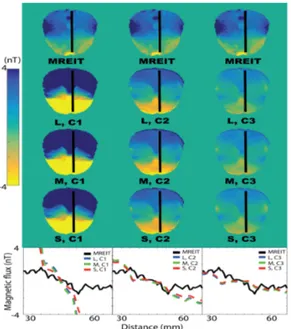
Christopher SaarMagnetic Flux Density Comparisons Between MREIT and FE Models. . . 31
Aprinda IndahlastariIn-vivo Projected Current Density Reconstruction: Comparisons Between MREIT and FE Models. 32 Neeta Ashok KumarCarbon electrodes for MREIT imaging of DBS current distributions. . . 33
Danyi ZhuComputer simulation of fast neural EIT in isolated retina. . . 34
Anna Witkowska-WrobelFeasibility of recording epilepsy changes with EIT and depth electrodes. . . 35
Sana HannanImaging Epileptic Activity in the Rat Brain with Three-Dimensional Electrical Impedance Tomography. . . 36
Kirill AristovichIn-vivo EIT imaging of spontaneous phasic activity in peripheral nerves. . . 37
Min H. KimHighly Reliable Iridium Oxide Electrodes for Electrical Impedance Tomography Imaging of Fast Neural Activity in the Brain. . . 38
Mayo FaulknerRecording thalamic impedance changes to assess feasibility of 3D EIT. . . 39
Nir GorenThe UCLH Stroke EIT dataset. . . 40
Ryan J. HalterEIT-based TBI Monitoring with Active and Passive Intracranial Electrodes. . . 41
James AverySimultaneous reconstruction of EIT and EEG. . . 42
Ilya TarotinModel of impedance change in unmyelinated fibres. . . 43
Andy AdlerCerebral perfusion imaging using EIT. . . 44
Barry J. McDermottA Novel Tissue-Mimicking Material for Phantom Development in Medical Applications of EIT. . . . 45
Rebecca J. YerworthDICOM for EIT. . . 46
Young Eun KimEIT based Natural Sleep Monitoring for Obstructive Sleep Apnea Patients. . . 47
Hyeuknam KwonQuantification of subcutaneous fat thickness using static EIT: experimental validation using ultrasound 48 Jianping LiApplication of electrical capacitance tomography on thrombus detection in blood extracorporeal circulation systems. . . 49
Yunjie YangTotal Variation and L1 Joint Regularization for High Quality Cell Spheroid Imaging Using EIT. . . 50
Benjamin SchullckeUsing a two plane EIT-System to reconstruct conductivity change in lung lobes. . . 51
Duc M. NguyenCombined electrical and thermal simulation of EIT to detect lesion formation in RF ablation using internal electrodes. . . 52
Min XuVarious electrode configurations for in-depth detection of electrical impedance mammography (revised). . . 53
Seward B. RutkoveEIT of muscle contraction: A preliminary study. . . 54
Gerald SzePreliminary volunteer experiment with an EIM system. . . 55
Richard BayfordNanoparticle Electrical Impedance Tomography. . . 56
Elyar GhalichiHeat Analysis in Magneto-Acousto Electrical Impedance Tomography. . . 57
Nima SeifnaraghiEstimation of Thorax Shape for Forward Modelling in Lungs EIT. . . 58
Sarah BuehlerLocalizing the aorta by electrical impedance tomography within regions of interest. . . 59
Alistair BoyleAn Embedded System for Impedance Imaging of Permafrost Changes. . . 60
Miguel-Ángel San-Pablo-JuárezImprovement of an EIT backprojection image using a bilateral filter. . . 61
Yunjie YangOptimal Design of a Planar Miniature EIT Sensor for 3D Cell Imaging. . . 62
Andy AdlerEIDORS Version 3.9. . . 63
Hancong WuA simplified calibration method for multi-frequency EIT system. . . 64
Marlin R. BaidillahUpper Arm Imaging based on Electrical Capacitance Tomography. . . 66
Sabine Krueger-ZiolekUsing EIT derived parameters for the detection of changes in work of breathing during spontaneous breathing. . . 67
Calvin EiberMicroelectrode array EIT in the deep brain: a feasibility study. . . 68
Thomas DowrickImprovements to the ScouseTom EIT System Arising From Noise Analysis. . . 69
Florian ThürkElectrical Impedance Tomography Image Explorer. . . 70
Ali ZarafshaniQuantitatively Assess Breast Density as a Cancer Risk Prediction Factor Using Electrical Impedance Spectrums. . . 71
Tae San KimPreliminary test of mobile body composition analyser using AFE4300. . . 72
Andy AdlerOrigins of Cardiosynchronous Signals in EIT. . . 73
You Jeong JeongPiezo-electric Nanoweb based Pressure Distribution Sensor for Detection of Dynamic Pressure. . . 74
Andy AdlerEfficient computations of the Jacobian matrix using different approaches are equivalent. . . 75
Nitish KatochMRCI: a toolbox for Low-frequency Conductivity and Current Density Imaging using MRI. . . 76
Taweechai OuypornkochagornImaging of Transient Hyperaemic Response (THR) by EIT. . . 77
Gerald SzeEnhancement of EIM system with shifting drive-receive method. . . 78
Alistair BoyleInternal Diode for Frequency Selective EIT Contrasts. . . 79
Mary McCrearyAccessible Multi-Frequency Screen for the Prognosis of Neuromuscular Atrophy and Degeneration. . . . 80
Andy AdlerFocusing electrical current at depth for ablation. . . 81
Acceleration of EIT Image Reconstruction on GPUs
Andrea Borsic
1, Michael G Crabb
2and William RB Lionheart
21NE Scientific LLC, MA, USA, [email protected]
2School of Mathematics, University of Manchester, UK, [email protected] Abstract: Graphic Processing Units (GPU) are highly
parallel architectures used in scientific computing to achieve substantial speed gains. This manuscript reports results from acceleration of EIT image reconstruction using GPUs, with gains of up to 24 times compared to EIDORS Version 3.8 running on a modern CPU under MATLAB. These gains enable a more interactive reconstruction on dense 3D meshes.
1
Introduction
A current trend in biomedical EIT research is the use of dense 3D FEM meshes in forward modelling to better represent the anatomy of interest. In part this trend is driven by approaches where CT, MRI, or Ultrasound images are used to build accurate models. Use of optical scanners for capturing the body shape has also been demonstrated [1]. The anatomically accurate meshes that result from these modelling approaches typically have between 100K and 300K nodes and 500K to 1M tetrahedral mesh elements. Non-linear image reconstruction on meshes of this size requires currently in excess of tens of minutes, therefore limiting the interactive exploration of data. The use of GPUs for accelerating EIT reconstruction has therefore been considered promising for some time [2]. In this manuscript computational speed-ups are reported for a complete implementation of EIT reconstruction on GPUs.
2
Methods
A forward solver implementing the complete electrode model, routines for computing the Jacobian matrix, routines for estimating the conductivity update with the Newton Raphson method, and with the PD-IPM framework [3] have been implemented on a GPU using the Thrust, CUSP, cuBlas, cuSparse libraries and a number of custom CUDA kernels. This low-level implementation compiles under Windows and Linux operating systems and results in a dynamic linked library (DLL). To facilitate the use, the DLL has been wrapped with Python/NumPy, exposing the functionality of the library to the high level Python language, resulting in a computation environment for EIT not too dissimilar to MATLAB. EIDORS [4] Version 3.8 was used as a reference implementation to test the GPU library against. Firstly the GPU library was tested for accuracy. It was verified that all the output from the relevant routines agreed to the outputs from EIDORS to 6 decimal places.
Secondly 3 meshes with 29K, 79K, and 190K nodes were generated in order to evaluate the performance of the GPU implementation against EIDORS running on a CPU. For each of these three meshes used for forward solving, 3 levels of coarse discretization were setup, resulting in 900, 3100, and 7275 parameters to estimate.
EIDORS timing data was collected under MATLAB Version 2016b on Ubuntu Linux 16.04 64bit on a computer with an Intel Core-i7 4790K CPU running at 4.0GHz, and 16GB of RAM. An inhomogeneous conductivity was used to generate synthetic measurements, which were later reconstructed with the Newton-Raphson algorithm, set to perform 6 iterations. The same setup was used for the GPU Library, which was run on the same computer, using an NVIDIA GTX TITAN Black GPU with 6GB of RAM. The same coarse-to-fine interpolation and regularization matrices were used to run the two algorithms. Table 1 reports speed-gain results. Time gains are very modest on the smaller mesh (1.42 to 2.49) as the setup and communication times on the GPU are significant compared to the overall reconstruction time. Timing results on the intermediate Mesh_2 (79K nodes) show increased benefit of GPU acceleration. On the larger Mesh_3 gains are significant, and range between 16.5 to 24.5 times depending on coarse resolution. Specifically the six non-linear reconstruction steps completed in 43 to 63 seconds on the GPU, depending on the coarse resolution level, and in 17 minutes in EIDORS on the CPU.
3
Conclusions
Use of GPU enables more interactive EIT image reconstruction. Further speed gains are expected from optimization of the current GPU library as well as when the upcoming Pascal family of GPUs are released.
References
[1] Forsyth, J., et al. "Optical breast shape capture and finite-element mesh generation for electrical impedance tomography" Physiological measurement 32.7, 2011.
[2] Borsic, A., E. A. Attardo, and R. J. Halter. "Multi-GPU Jacobian accelerated computing for soft-field tomography" Physiological measurement 33.10, 2012.
[3] Borsic, A., and A. Adler. "A primal–dual interior-point framework for using the L1 or L2 norm on the data and regularization terms of inverse problems" Inverse Problems 28.9, 2012.
[4] Adler, Andy, et al. "EIDORS Version 3.8." Proc. of the 16th Int. Conf. on Biomedical Applications of Electrical Impedance Tomography. 2015.
Table 1: Speed gains for three different forward mesh densities and for three different level of coarse discretisation. GPU speed gains are limited for small meshes, but significant (16 to 24 times) for dense meshes.
Mesh_2 29K Nodes Mesh_2 79K nodes Mesh_3 190K nodes 900 Inv. Parameters 2.49 speed gain 8.20 speed gain 24.46 speed gain 3,100 Inv. Parameters 1.42 speed gain 5.12 speed gain 18.02 speed gain 7,275 Inv. Parameters N/A 5.09 speed gain 16.55 speed gain
Towards Efficient Iterative Absolute EIT
Henry FJ Tregidgo
1,2, Michael G Crabb
1, William RB Lionheart
11University of Manchester, Manchester, UK. 2[email protected]
Abstract:One factor limiting the use of absolute reconstruc-tions in 3D lung EIT is the computational cost of iterative algorithms. We show how the programming experience of the Finite Element and Research Software Engineering commu-nities can be applied to these algorithms, resulting in a speed up of reconstructions in EIDORS 3.8 [1]. We also outline a combination of absolute and difference imaging to provide fast pseudo-absolute imaging.
1 Introduction
In situations where 3D absolute EIT could be useful the high cost of iterative inversion can be prohibitive. A large propor-tion of time taken is in the solupropor-tion of a sparse linear system representing the forward problem [2]. We present simple soft-ware refinements to improve performance of this linear solve in Matlab. We also address refinements in construction of the Jacobian, coarse-to-fine and Laplace-prior matrices.
For purposes such as parameter fitting and control of ven-tilation, absolute reconstruction is only required for calibra-tion [3]. For situacalibra-tions where calibracalibra-tion of absolute values is required at multiple time steps, we present a combination of absolute and difference imaging to provide a fast pseudo-absolute reconstruction.
2 Reconstruction Steps
Errors in floating point arithmetic can produce small asym-metries even when using seemingly symmetric constructions of the system matrix. For example the factorisation of the FEM system matrix for piecewise linear elements into mesh and conductivity dependent components [4] as performed in EIDORS. This asymmetry, shown in Figure 1, can cause checks in default sparse linear solvers to incorrectly choose slower non-symmetric algortithms. In particular the UMF-PACK algorithm is chosen over CHOLMOD by MATLAB’s mldividefunction, resulting in worse performance.
We demonstrate how symmetry correction can drastically reduce the sparse linear solve time as shown in Table 1. We additionally detail other software engineering refinements to speed up construction of the Jacobian, coarse-to-fine and Laplace-prior matrices. These include vectorisation of opera-tions, replacement offindoperations withsortfunctions and reduction of complexity through further use of symmetry.
Figure 1:Sparsity pattern for the antisymmetric system matrix error component using first order elements. Entries are of order 10−12.
3 Pseudo-absolute Reconstruction
We propose using additional imaging modalities to produce a segmented mesh of the thorax [5, 6] and performing a very low dimensional absolute reconstruction of a single frame on this mesh. The absolute values are then incorporated into the conductivity Jacobian for further difference imaging. This re-sults in improved residual data-fit and only requires a small additional offline processing time. Using the 46k node mesh from Table 1 for a simulated domain with 64 electrodes and 5 level set regions required an additional 2 minutes elapsed time with the improvements from the previous section.
4 Conclusions
By ensuring conditions are met for the use of the optimal linear solvers, and reducing the dimensionality of the itera-tive inversion, significant speed-ups are available and pseudo-absolute reconstructions are possible.
5 Acknowledgements
The authors would like to thank A. Boyle and A. Adler for their help in confirming these efficiency savings in EIDORS.
References
[1] Adler A, Boyle A, Crabb MG, et al. InProc. 16th Int. Conf. Biomed. Applications of EIT. 2015
[2] Boyle A, Borsic A, Adler A.Physiol Meas33(5):787, 2012
[3] Tregidgo HFJ, Crabb MG, Lionheart W. InProc. 16th Int. Conf. Biomed. Applications of EIT, 96. 2015
[4] Vavasis SA.SIAM J on Numerical Analysis33(3):890–916, 1996 [5] Crabb M, Davidson J, Little R, et al.Physiol Meas35(5):863, 2014 [6] Grychtol B, Lionheart WR, Bodenstein M, et al.Medical Imaging, IEEE
Transactions on31(9):1754–1760, 2012
Table 1: Time comparisons for symmetric and non-symmetric linear solve on two meshes of the same thorax segmentation. Timings are given in both CPU and elapsed time as measured on a 2.8GHz Intel Core i7 with 16 GB 1.6 GHz DDR3 RAM.
N. nodes Unsymmetric Symmetric Speedup Unsymmetric Symmetric Speedup
(CPU time s) (CPU time s) (CPU time×) (elapsed time s) (elapsed time s) (elapsed time×)
46k 9.83 3.47 2.83 6.55 1.09 6.03
Rotational electrical impedance tomography with few electrodes
Mari Lehti-Polojärvi
1*, Olli Koskela
1*, Aku Seppänen
2, Edite Figueiras
3and Jari Hyttinen
1 1BioMediTech Institute and Faculty of Biomedical Sciences and Engineering, Tampere University of Technology, Tampere, Finland,[email protected], [email protected]
2Department of Applied Physics, University of Eastern Finland, Kuopio, Finland 3 International Iberian Nanotechnology Laboratory, Braga, Portugal
* with equal contribution Abstract: In multimodal applications, electrodes used in
electrical impedance tomography (EIT) should cover only part of the object surface to allow the use of other probes. We propose to use a rotational setup with only eight electrodes. To obtain a proof of concept of this method, we measured gelatin phantoms with resistive inclusions. The results proof the method provides images of good quality.
1
Introduction
Placing EIT electrodes so that they cover only a limited portion of the object surface would save space for other probes, enabling multimodal imaging. For this purpose, we propose a method applying eight fixed electrodes around a rotating object. Our goal is to use this method for monitoring cell cultures in a cylindrical hydrogel scaffold.
Aim of this study is to demonstrate the effectiveness of the proposed method by phantom measurements.
2
Methods
2.1 Rotational setup
We used two sets of four electrodes placed symmetrically on opposite sides of the object as is shown in Fig. 1. Each set covered one quarter of the sample boundary (90 degrees). To be able to rotate the object while keeping the electrodes fixed, we used a thin layer of aqueous solution between the object and the electrodes.
2.2 Rotational reconstruction
For each rotated measurement position, we defined a linear mapping of the conductivity distribution from initial position to the rotated coordinates. These mappings were incorporated into the forward model of EIT. Inverse of this model was used to reconstruct the conductivity distribution within the object, corresponding to the set of voltage measurements in these rotated measurement positions. All computations were performed in MATLAB with an adaption of the open source EIDORS package. [1]
2.3 Experiments
Cylindrical gelatin phantoms were measured before and after adding resistive inclusions with different sizes. The phantoms were manually rotated and measurements recorded every 5.6-degree turn, providing data from 64 different angles. The measurements were done in a 16-electrode tank (used previously for example in [2]) where eight electrodes were insulated and eight were in use. The measurement device was KIT4, presented in [3]. All measured phantoms were constant along the height of the tank, thus analysis in two dimension is adequate.
3
Results
Difference mode reconstructions of one of the experiments are shown in Fig. 1. Rotational data from the object enhances image quality.
4
Conclusions
This study demonstrates that rotational EIT provides good image quality even with limited electrode coverage on the object. We anticipate this method could create new applications of EIT imaging.
5
Acknowledgements
Financial support has been provided by Jane and Aatos Erkko foundation, Instrumentarium Science foundation, Tekes Human Spare Parts project and Academy of Finland. Authors would like to thank Tuomo Savolainen and Panu Kuusela (University of Eastern Finland) for the help in the laboratory measurements.
References
[1] A Adler, W Lionheart,PhysiolMeas, 27: S25–S42, 2006 [2] D Liu, V Kolehmainen, S Siltanen, A Laukkanen, A Seppänen,
Inverse Problems and Imaging,9: 211-229, 2015
[3] J Kourunen, T Savolainen, A Lehikoinen, M Vauhkonen and L Heikkinen,MeasSciTechnol, 20, 2009
Figure 1: A photo of the measured object (left) and corresponding reconstructions using data from 1 (middle) and 64 (right) rotational positions. Setup includes a tank with eight electrodes in use (numbers 1-8), a platform for rotation (white), aqueous solution around a rotating gelatin object and a resistive plastic tube (white circle).
Spatio-Temporal Regularization over Many Frames
Alistair Boyle
University of Ottawa, Ottawa, Canada,[email protected] Abstract:Regularizing over both spatial and temporal spaces
for EIT data can lead to very large matrices which can be chal-lenging to compute. The Kronecker product identity may be leveraged with the Conjugate Gradient method to construct a system of equations that scales linearly with the number of data frames collected and reconstruction parameters.
1 Introduction
Gauss-Newton methods are generally used to reconstruct an Electrical Impedance Tomography (EIT) conductivity image for a single frame of data. Multiple frames of data may be reconstructed together and have regularization applied across them, leading to spatio-temporal regularization.
2 Gauss-Newton
The Gauss-Newton iterative update (GN-update) is
xn+1=(J2+λR2)−1 JTWb+λR2(x∗−xn) (1) whereJ2 =JTWJandR2 =RTR. New parametersxn+1
are calculated using results from iterationnand with a prior estimatex∗, where the JacobianJis calculated based onxn, the measurements are weighted by an inverse noise covari-ance matrixW, and the reconstruction is regularized byR
with a hyperparameterλcontrolling regularization strength. Following [1], the GN-update (1) may be expanded as a block-diagonal matrix to handle many frames in a time-series of data and reconstruct these frames simultaneously while ap-plying regularization across time. Entries in the time series are assigned an exponential smoothing Γ, so that adjacent
frames are assumed to be strongly correlated. The same spa-tial regularizationRis applied to every frame’s reconstruc-tion. I⊗J= J J J Γ⊗R= RRR RRR RRR (2) The GN-update becomes
vec(Xn+1) = (I⊗J)T(I⊗W)(I⊗J)+
λ(Γ⊗R)T(Γ⊗R)−1 (I⊗J)T(I⊗W)vec(B)+
λ(Γ⊗R)T(Γ⊗R)vec(X∗−Xn) (3) whereX denotes the reconstruction parameters joined into a matrix with one column per frame and the vec()operator reshapes this matrix into a single column vector. The mea-surementsBare treated similarly. Using Kronecker product
identities, (3) may be written
vec(Xn+1) = (I⊗J2+λΓ2⊗R2)−1
I⊗(JTW)vec(B) +λΓ2⊗R2vec(X∗−Xn) (4) whereΓ2 =ΓTΓ. This formulation can result in very large,
dense matricesI⊗J2. The Wiener filter form, as suggested
in [1], may help though it still gives the large dense matrices.
1 10 0.1 1 10 100 Gauss-Newton Conjugate Gradient 132.3 s 0.41 s Frames Runtime (s)
Figure 1:Runtime for a 16 electrode 2D Finite Element mesh (1600 elements) for 1 to 20 frames of 208 measurements using Gauss New-ton (GN) (4) and Conjugate Gradient (CG) (7); CG scales to many frames of measurement data while GN runs exponentially slower as more frames are added
3 Conjugate Gradient
The Conjugate Gradient (CG) update [2] efficiently calculates the inverse in (4) by iterative evaluation of
(I⊗J2+λΓ2⊗R2)vec(Xn+1) =
I⊗(JTW)vec(B) +λΓ2⊗R2vec(X∗−Xn) (5) A key identity of the Kronecker product may be used to sig-nificantly reduce the computational requirements
vec(AXB) =vec(C) = (BT⊗A)vec(X) (6) which transforms (5) into
vec(J2Xn+1+λR2Xn+1ΓT2) =
vec JTWB+λR2(X∗−Xn)ΓT2
(7) where, by judicious choice in the order of operations, one can maintain a minimal storage footprint. Note that in the GN solution, solving (5) would result in the same very large ma-trices as (4), while for CG the Kronecker products do not need to be expanded.
The CG method typically computes the solutionXn+1to
a certain precision. For ill-posed problems, the accuracy of the parametrization is limited by measurement noise and reg-ularization. Stopping the conjugate gradient iterations early avoids getting trapped in fruitless iterations. Rigorously CG stopping criteria for EIT CG-updates have been developed in [3], but were heuristically found in this work through plotting of the CG error estimates. Halting CG iterations when the algorithm started to oscillate gave nearly identical results.
4 Discussion
Spatio-temporal regularization combining the techniques de-scribed in this work, the Kronecker product identities and the Conjugate Gradient method, may be brought together to tackle previously uncomputable EIT data sets.
References
[1] Dai T, Soleimani M, et al.Med Biol Eng Comput46(9):889–899, 2008 [2] Shewchuk J. An introduction to the conjugate gradient method without
the agonizing pain. Tech. rep., Carnegie Mellon University, 1994 [3] Rieder A.SIAM J Numer Anal43(2):604–622, 2006
Image reconstruction in Lorentz force Electrical Tomography
Nick Polydorides
School of Engineering, University of Edinburgh, Edinburgh, UK,[email protected] Abstract: We describe an algorithm for electrical
conduc-tivity reconstruction from Lorentz force Electrical Impedance Tomography data. The inverse problem is formulated in three iterations, beginning with the recovery of the curl of the cur-rents within the body, and subsequently reconstructing the current density and the conductivity. Subject to the appropri-ate acoustic modulation the method yields quantitative, stable and high resolution imaging.
1 Introduction
Lorentz Force Electrical Impedance Tomography (LFEIT) [1], also known as Magneto-Acousto-Electric Tomography[2], has recently emerged as an alternative modality that can yield, in principle, noise-robust, high-resolution, quantitative conductivity imaging. The technique is primarily destined for early stage cancer detection coupling the resolution of ultrasound imaging and the sensitivity of EIT to small cancer lesions. The LFEIT measurements are acquired on a pair of electrodes attached to the boundary of a conductive body Ω, homogeneous in density ρand speed of sound c, whilst in a static magnetic field with strength
B. An ultrasound wave is then driven into the body per-turbing the conductive tissue which in turn yields an interior Lorentz force current, leading to Ohmic currents and poten-tials. The measurement admits a simpler expression via its adjoint model. Ifv= 1
ρgradϕfor a velocity potentialϕ (sat-isfying the wave equation) andJais the current density of the boundary adjoint source corresponding to the measurement electrodes then the measurement is approximately
M(t)≈ −1
ρ Z
Ω
dr B· ϕ(t) curlJa(t), (1) where the sought conductivity information is encoded into curlJa=−gradσ× gradwwithwthe adjoint potential.
2 Image reconstruction
We outline the image reconstruction algorithm for recon-structing the conductivityσfrom LFEIT data captured on two pairs of electrodes. In this context, quantitative imaging re-quires, in addition, two impedance measurements on the same electrodes. The image reconstruction process, as originally suggested in [2] involves 3 iterated inverse problems, in prin-ciple all stable, subject to having sufficient data. We outline these stages that take LFEIT data to the interior curl of the ad-joint current densities, then the curls to the currents and finally reconstructing the conductivity from the currents.
2.1 Reconstructing the adjoint curl
If the acoustic velocity potential is focused at a point within the region, say through linear phased array-based ultrasound focusing, repeating the measurements for three orthogonal
magnetic field directions yields a representation of the curl there.
2.2 Reconstructing the adjoint current density
Having reconstructedcurlJaon a dense grid of points within the domain we can then compute the current density from the solenoidal condition divJa = 0 and the fact that the current density is a smooth, continuous field that can be ex-pressed as a sum of a solenoidal and a conservative field
Ja= curlK
−gradφfor a unique combination ofKandφ. 2.3 Reconstructing the conductivity
The final step of the reconstruction process is a current-density impedance imaging imaging problem, for which we develop an adaptation of the J-substitution algorithm [3] to exploit the information on the recovered vector fieldJa. As current density resolves the conductivity distribution up to a multiplicative constant, having two distinct currents and their respective impedance measurements (i.e. say on three elec-trodes) provides the necessary information to image the con-ductivity. The results shown below were obtained with sim-ulated data containing 5% additive noise. To make the com-parison between target and image more profound we plot the logarithm of the images at the same cross section of a 3D phantom.
,
Figure 1: Cross section of the logarithm of the conductivity in the target (left) and reconstruction (right) form an ellipsoidal breast phantom at heightz = 3cm. Note the very small reconstruction error.
3 Conclusions
Our numerical results support the claim that despite the com-plicated experiment setup of LFEIT, image reconstruction is stable and the images provide adequate spatial resolution for medical diagnosis.
References
[1] P. Gransland-Mongrain, J-l. Mari, J-Y. Chapelon and C. LafonIRBM 34(4-5), p. 357-360, 2013.
[2] L KunyanskyInverse problems, 28, 2012.
[3] O. Kwon, EJ. Woo, JR. Yoon and JK. Seo,IEEE Trans Biomed Eng., 49(2), p.160–167, 2002.
Fused-data Transrectal EIT incorporating Biopsy Electrodes
Ethan K. Murphy
1, Xiaotian Wu
1, and Ryan J Halter
1,21Thayer School of Engineering, Dartmouth College, Hanover, NH, USA, [email protected] 2Geisel School of Medicine, Dartmouth College, Hanover, NH, USA
Abstract: This work explores fusing transrectal electrical impedance tomography (TREIT) data from the top surface of an ultrasound probe and 4 electrodes from a biopsy needle measured at different positions to produce an
improved reconstruction. Sensitivity analysis and
measured tank experiments are used to validate the approach. This fused-data TREIT method has significant promise for improving prostate cancer screening.
1
Introduction
Detecting prostate cancer non-invasively is clinically challenging. Low threshold PSA-based screening has a high sensitivity, but low specificity due to numerous benign reasons for elevated levels [1]. Men with elevated levels of PSA are typically subject to image-guided biopsy protocol for more accurate diagnosis. Unfortunately, numerous investigators report that transrectal ultrasound (TRUS)-guided biopsies miss 10-30% of all cancers [1]. A number of ex vivo studies have shown that electrical properties show significant differences between benign and cancerous tissues [2], and there has been prior work in developing transrectal electrical impedance tomography (TREIT) algorithms [3] that include a biopsy needle electrode [4]. This study builds on [4] by fusing TREIT and biopsy electrodes measurements from different positions to increase the sensitivity far from the TRUS probe.
2
Methods
The fusion approach is based on a standard Gauss-Newton algorithm using a regularization scheme optimized for open domains [5]. In the experiment illustrated in Fig. 1A the TRUS probe with biopsy electrode is held fixed while a tank and two metal inclusions are rotated 0 to 340o in 20o
steps. The biopsy electrodes are approximately 37 mm in front of the TRUS probe and are at the same depth as the inclusions.
The fusion process utilizes a single finite element method (FEM) mesh that has the TRUS probe and biopsy needle encoded within the domain. The mesh constructed in gmsh has ~500k nodes and ~3M elements. Corresponding to each tank rotation the mesh is rotated to yield the same relative geometry as the experiment and the Jacobian is calculated using a dual mesh approach. The dual mesh approach maps the fine (and dense) FEM mesh onto a much coarser set of nodes in which the reconstruction is actually performed. The same set of coarse nodes is used for each rotation, i.e. the coarse nodes remain fixed while the FEM mesh rotates. There are 1,778 coarse nodes in a cylindrical region extending from 25 to 50 mm in front of the TRUS probe with a radius of 10 mm. The measurements and Jacobians are concatenated so the problem can be solved as if it were a standard EIT problem [6].
A difference reconstruction using this fused data
approach is shown in Fig. 1B. The yellow ‘blocks’
represent coarse nodes that are > 0.85 the maximum of the reconstruction, i.e. it represents the reconstructed metal inclusions. We used a Tikhonov factor of 1e5 and tetrapolar patterns that had 2 electrodes on the biopsy needle and 2 electrodes from the TREIT electrode array, as these patterns were agreed well with simulation on a blank tank and gave a large region of sensitivity based on an analysis of the Jacobian.
Figure 1: A. Downward view of TRUS probe with TREIT array (in green), biopsy needle and electrode on the left, and two metal inclusions in a saline filled tank on a rotation stage, and B. a difference reconstruction that fused the rotated datasets where the yellow represents nodes that are > 0.85 the maximum, the red spheres represent the true solutions of the inclusions, and the blue surface are faces of the FEM mesh.
3
Conclusions
This work presents a proof of principle difference reconstruction from tank experiment that shows that fused data in this TREIT with biopsy electrode is possible. In ongoing work more general rotations and translations of the probe and biopsy needle are being considered, which are further important steps to bringing this technique into a clinical setting.
4
Acknowledgements
This work was supported in part by the U.S. National Institutes of Health under Grant 1R01CA143020–01A1 and DoD CDMRP Grant W81XWH-15-1-0102.
References
[1] Campbell's Urology, 9th ed, P. Walsh, Editor. 2007, Saunders: Philadelphia
[2] R. J. Halter, et al., IEEE Trans. Bio. Eng., 54:,1321-1327, 2007. [3] A. Borsic, et al., Phys. Meas., 30:S1-S18, 2009.
[4] Y. Wan, et al., 34th Annual Intern. Conf IEEE EMBS, 6220-6223, Sept. 2012.
[5] E.K. Murphy, A. Mahara, R.J. Halter, IEEE Trans Med. Imag., 35:1593-1603, 2016.
[6] E.K. Murphy, A. Mahara, R.J. Halter, IEEE Trans Med. Imag., 36:892-903, 2017.
Convergence of finite element approximation in electrical impedance
tomography
Erfang Ma
11Department of Mathematical Sciences, Xi’an Jiaotong-Liverpool University, Suzhou, Jiangsu Province, China, [email protected]
Abstract: For electrical impedance tomography (EIT) with the complete electrode model, we prove that the estimated voltages on the electrodes by the finite element method (FEM) converge pointwisely to the true ones as the sizes of elements in the underlying mesh approach zero.
1 Introduction
Assume the conductivity distributionσof a convex polygonal regionΩis of interest.Lelectrodes are placed on the bound-ary ofΩ. Fori= 1,2, ..., L,Iiis the amount of current flow-ing into the region through thei-th electrode; Uiis the volt-age on thei-th electrode;eiis the part of boundary ofΩthat is covered by thei-th electrode; ziis the contact impedance underneath thei-th electrode. U = (U1, U2, ..., UL)T ∈RL. The potential distribution overΩis denoted byuwhich is as-sumed to belong to Sobolev spaceH1(Ω).H def= H1(Ω)⊗RL i.e., the Cartesian product ofH1(Ω)andRL.
Given the above assumptions, the weak formulation [1] for the boundary value problem of EIT is to find[(u, U)]in the quotient spaceH/Rsuch that
a([(u, U)],[(v, V)]) =hℓ,[(v, V)]i for all[(v, V)]∈H/R, (1) where a([(u, U)],[(v, V)])def= Z Ω σ∇u· ∇vdΩ + L X i=1 1 zi Z ei (u−U)(v−V)ds, (2) hℓ,[(u, U)]idef= L X i=1 UiIi. (3)
The spaceH/Ris associated with two different norms: k[(u, U)]kH/R def = inf c∈R ku−ckH 1(Ω)+kU−ckRL, (4) k[(u, U)]ka def = pa([(u, U)],[(u, U)]). (5)
2 Methods
AssumeH1h(Ω)is a finite element space forH1(Ω)based on a triangularizationThof domainΩ. Herehis a discretization
parameter. The(uh, Uh)∈Hh
def = H1
h(Ω)⊗RLis a finite el-ement solution. The[(uh, Uh)]is the element in the quotient spaceHh/Rthat corresponds to(uh, Uh). We claim
lim
h→0cinf∈RkU−Uh+ckRL= 0. (6)
Proof. According to the density argument [2] and the inter-polation theory for Sobolev space [3], for anyǫ >0, we can find ahand[(Ihv, U)]∈Hh/Rsuch that
lim
h→0k[(u, U)]−[(Ihv, U)]kH/R< ǫ (7)
wherev∈H2(Ω)andI
hv∈Hh1(Ω)is the interpolation ofv by a piecewise polynomial of degree one. This gives
lim
h→0[(vh,Vhinf)]∈Hh/Rk
[u, U]−[(vh, Vh)]kH/R= 0. (8) On the other hand, the Galerkin orthogonality [3] and the el-lipticity [1] of the bilinear form (2) lead to
k[(u, U)]−[(uh, Uh)]kH/R≤C inf
[(vh,Vh)]∈Hh/Rk
[(u, U)]−[(vh, Vh)]kH/R, (9) for some constantC. From (8) and (9),
lim
h→0k[(u, U)]−[(uh, Uh)]kH/R= 0. (10)
The (10) and (4) give (6).
3 Conclusions
For EIT, the finite element approximation for the voltages on the electrodes converge to the true ones as the size of elements in the underlying mesh tend to zero.
4 Acknowledgements
This work is supported by a research development fund from Xi’an Jiaotong-Liverpool University.
References
[1] E Somersalo, M Cheney, D IsaacsonSIAM J Appl Math, 52:1023–1042, 1992
[2] PG CiarletThe Finite Element Method for Elliptic ProblemsSIAM: Philadelphia, 2002
[3] D BraessFinite Elements: Theory, fast solver and applications in solid mechanicsCUP: New York, 2007
EIT in Multimodal Imaging for Avoiding Biopsies
of False Positive Results in Mammography
P. Robert Kotiuga
1 1Boston University, ECE Dept., 8 St. Mary’s Str., Boston, MA, USA, [email protected] Abstract: EIT, in the context of false positives in
mammography is considered where repeated negative results of biopsies can lead patients to avoid future mammograms. Our approach is to consider the conditional probabilities associated with use of EIT in conjunction to mammography, not for increasing the overall rate of detection of breast cancer, but for maintaining the best possible rate of cancer detection with fewer biopsies.
Introduction
Although EIT is a notoriously ill-conditioned problem, it has distinct advantages over other imaging modalities and it has made a place for itself in several multimodal medical imaging contexts. For example, forced lung ventilation in respiratory medicine where continuous monitoring of lung volume can be achieved for “lung protective ventilation strategy”, without resorting to repeated x-ray exposure[1]. Another context is cancer imaging where knowledge of the conductivity of tissue can help discard false positives. However, in the application of EIT to cancer imaging, the ill-conditioning of EIT and coregistration of data from different imaging modalities becomes a critical issue. Coregistration is particularly difficult to achieve in the context of mammography. By focusing on three dimensional reality of mammography, the eigenfunctions of the Dirichlet to Neumann(D-N), map as a means to deal with both ill conditioning and coregistration, the present work offers a means to reduce the number of false positives that require a follow-up biopsy. The drawback of the proposed work is that it requires a more personalized approach, and considerably more preparation on the part of the patient. Thus, it only makes sense for those with a history of false positives being discovered by means of a biopsy. This classic example of a “false positive paradox”[2] can deter people from having follow-up mammograms.
1
Methods
Key aspects to the proposed approach are:
1) Dealing with the underlying ill-conditioning in a manner that reflects the 3D reality of the problem. Specifically, despite the fact that EIT requires vastly more data as one goes up in dimension, one also has to take advantage of the fact that the conditioning of EIT also gets better as dimension increases[3]. This is
counterintuitive to many in the field who feel it is
necessary to first demonstrate EIT in lower-dimensional contexts which require less data. 2) The conditioning of EIT can also be improved
dramatically by reformulating EIT in terms of “Euclidean Dirac operators” and not in terms of the Laplace operator[4]. This aspect is best understood in terms of a “generalized Calderon problem” for self-adjoint elliptic operators. The underlying principles and the spectral theory of their associated “D-N” maps will be sketched in the extended paper.
3) Exploitation of generic properties of the eigenfunctions of the D-N map as a means to a personalized electrode configuration for coregistration of EIT data.
4) Articulating, the improvement in the conditioning and data acquisition in the context of a Bayesian framework where the conditional probabilities associated with avoiding a biopsy depends on the amount of coregistered data acquired.
2
Conclusions
This paper to considers the conditional probabilities associated with use of EIT in conjunction to mammography, not for increasing the overall rate of detection of breast cancer, but for maintaining the best possible rate of cancer detection with increased patient engagement and fewer biopsies. The underlying Bayesian model takes into account the dependence of the conditioning of the EIT problem as a function of dimension, and other aspects which affect conditioning.
3
Acknowledgements
The author is indebted Bill Loinheart for encouraging a broader exploitation of geometric insights in EIT practice.
References
[1] I. Frerichs, et. al., Chest electrical tomography examination, data analysis, terminilogy, clinical use and recommendations: Consensus statement of the Translational EIT development study group review. Thorax Online First, published on October 4, 2016 as
10.1136/thoraxjnl-2016-208357.
[2] B. L. Madison, Mathematical Proficiency for Citizenship, Chapter 8 in, A.H. Schoenfeld (Ed.), Assessing Mathematical Proficiency, MSRI Monograph No. 53, Camb U. Press, 2007
[3] P. R. Kotiuga, A Rationale for Pursuing EIT and MREIT in 3-D based on Weyl Asymptotics and Problem Conditioning. EIT 2008 Conference, Dartmouth College, Hannover NH, June 16-18, 2008. [4] Kotiuga, P.R., Metric Dependent Aspects of Inverse Problems and Functionals Based Helicity. Journal of Applied Physics, 70(10), May 1993, pp. 5437-5439.
Direct Absolute EIT Imaging on Experimental Data
Sarah Hamilton
11Department of Mathematics, Statistics and Computer Science, Marquette University, Milwaukee, WI, USA, [email protected]
Abstract: A direct reconstruction algorithm [1, 2] for 2D Absolute Admittivity EIT imaging is presented and demon-strated on experimental tank data for the first time. The key benefit of the method is that it does not require any simu-lated reference dataΛ1orΛref. The method is based on the
D-bar methodology which uses a tailor-made nonlinear Fourier transform of the measured boundary voltage/current dataΛγ to uniquely recover the admittivityγ=σ+iωǫof the interior.
1 Introduction
In Electrical Impedance Tomography (EIT) electrical mea-surements are taken on electrodes at the body’s surface, and a mathematical inverse problem is solved to recover the inter-nal conductivity/admittivity of the body. The most common solution methods solve an optimization problem to minimize the error between measured and predicted data (e.g. volt-age/current data) therefore requiring a finely-tuned forward model. By contrast, D-bar methods solve the inverse problem directly without repeated forward solutions.
D-bar methods are based on using a nonlinear Fourier transform of the Dirichlet-to-Neumann (voltage-to-current-density) data that is tailor-made for the EIT problem. The con-ductivity/admittivity is then recovered from the transformed data by solving a∂k(D-bar) equation in the transformed vari-ablek. While there are multiple D-bar methods for EIT, they all have the same basic form:
Current/Voltage
data −→ Scatteringdata −→ Conductivity/Admittivity
2 Methods
Here we use a specific D-bar method that is based on intro-ducing an auxiliary parameterk ∈ Cand transforming two special complex geometrical optics (CGO) solutionsu1 and
u2of the admittivity equation
∇ ·γ(z)∇u(z, k) = 0, z∈Ω⊂R2 (1)
into a first-order matrix system of CGOs:
[−Dk+Q(z)]M(z, k) = 0 (2) whereDkM = ¯ ∂z 0 0 ∂z M−ik 1 0 0 −1 0 M12 M21 0 andQ(z) = 0 −12∂zlogγ(z) −1 2∂¯zlogγ(z) 0
. These CGO
so-lutions satisfy a D-bar equation in the transform variablek
∂kM(z, k) =M(z,k¯) e(z,k¯) 0 0 e(z,−k) S(k), (3) from which the admittivityγcan be recovered.
This work uses a ‘Born’-approximation to the scattering dataS(k)that can be computed directly from the measured dataΛγvia: S12(k) = i 4π R ∂Ωe− i¯kz(Λ γ+i∂τ) e−ikz¯ −ik ds(z) S21(k) = − i 4π R ∂Ωe i¯k¯z(Λ γ−i∂τ) eikz ik ds(z), (4)
where ∂τ denotes the tangential derivative operator: ∂τf(z) = ∇f(z)·τ and the asymptotic behaviors ofu1 ∼
eikz
ik andu2∼ e−ik¯z
−ik are used [1, 2].
Figure 1 demonstrates the method on archival experimen-tal tank data taken on RPI’s ACT3 EIT system, and compares the results to those from the traditional formulation [3] for dif-ference and absolute imaging for the first-order system D-bar method (2).
3 Conclusions
A D-bar method that does not require any simulated mea-surement dataΛ1 to form absolute EIT images is presented
and demonstrated on experimental data for the first time. The method is non-iterative, trivially parallelizable, and holds for both conductivity-only as well as admittivity imaging. If only the conductivity is desired, symmetries in the underlying CGO system (2) can be exploited reducing the computational load by a factor of 1/2 leading to an even faster solution.
4 Acknowledgements
The experimental data was provided by the EIT lab at RPI, for which we express our thanks.
References
[1] C.N.L. Herrera,PhD Thesis, Escola Politécnica da Universidade de São Paulo, 2012.
[2] C.N.L. Herrera, M.F.M Vallejo, J.L. Mueller, R.G. LimaIEEE TMI, 34(1): 267-274, 2015.
[3] S.J. Hamilton, C.N.L. Herrera, J.L. Mueller, A. Von HermannInverse Problems28: 095005, 2012. EXPERIMENT DIFFERENCE IMAGE TRADITIONAL ABSOLUTEIMAGE NEW ABSOLUTEIMAGE
Figure 1: Comparison of D-bar methods on experimental data. Note that the difference image requiresΛγ−Λref, the traditional absolute image [3] requiresΛγ−Λ1whereΛ1is simulated, however the new absolute image (right) only requires the measured dataΛγ.
EIT reconstruction regularized by Total Generalized Variation
Bo Gong, Benjamin Schullcke, Sabine Krueger-Ziolek, Knut Moeller
Institute of technical Medicine (ITeM), VS-Schwenningen, Germany, Abstract: EIT reconstructions with Total Variation (TV)
regularization promote solutions with sparse first order derivation. Consequentially, the sharp boundaries between different tissues can be approximated. However, TV regularization may induce blocky images which are not realistic in clinical applications. To reduce such blocky artefacts, we applied the Total Generalized Variation (TGV) for regularization. TGV employs higher order differential operators over the finite element mesh.
1 Introduction
We focus on the linearized time difference lung EIT reconstruction. The image reconstruction intends to solve the conductivity changes from the measured voltage differences between two time steps. This is an ill-posed inverse problem which needs regularizations to confine the solution space. Mathematically, the following regularized optimization problem is solved:
(1) where is the Jacobian matrix, is the regularization term and is the regularization parameter.
One type of regularization term is TV regularization. It is the norm of the first order derivation of underlying conductivity distribution over the domain. Because of the norm in TV regularization, the TV regularized EIT reconstruction promotes a solution with sparse discrete derivation of the underlying solution. Consequentially, TV regularization identifies the sparse sharp interfaces between different tissues and promotes block-wise constant image reconstruction. As a side effect, the reconstructed images often contain the blocky artefacts. To reduce these blocky artefacts, higher order differential operators are considered in regularization, such as the total generalized variation regularization TGV [1].
2 Methods
EIT images are reconstructed under the finite element mesh (FEM) framework. An FEM can be endowed with an undirected weighted graph structure: , which contains three components: a set that consists of the indexed vertices, a set of edges and a weighted adjacency matrix . Explicitly, each finite element in FEM is identified as a vertex in and two vertexes and in are connected by an edge if the corresponding two finite elements share a common boundary. A weight which equals the area of the shared boundary is attributed on each edge . These weights are saved as the -th entry of the adjacency matrix . The differential operator of the functions over the undirected graph is indeed the weighted indication matrix :
(2).
With this formulation, the TV regularization on the graph structured FEM framework is represented by: . On the other hand, following [2], the total generalized variation operator is defined by:
. (3) Intuitively, is an approximation of the first order derivation of and is an approximation of the second order derivation of . Under the TGV regularization, the reconstruction is to solve the follow optimization problem:
. (4)
We solve this problem by Split Bregmann iterations [3].
3 Conclusions
The performance of different regularization methods has been compared by 2.5D simulations (Fig. 1). The simulated voltage difference was added with 10% white noise. The common parameters for TV and TGV regularizations are same and were heuristically chosen. It can be observed that the reconstruction with TGV regularization recovers the piecewise linear conductivity distribution. However, TGV regularization fails to smooth out the overshoots introduced by the fidelity term. This leads to the artefacts at the interfaces between contrasts.
Figure 1: Example reconstructions with different regularization methods. The reconstructed located on a vertical line cut (black line in Ground Truth) are demonstrated in the lower right plot.
4 Acknowledgements
This work was supported by the BMBF grant no. 03FH038I3 (MOSES).
References
[1] K Bredies, K Kunisch, and T Pock SIAM J. Imaging Sci., 3(3), pp. 492 526
[2] S Ono, I Yamada, and I Kumazawa Conf ICASS, 2015 [3] T Goldstein, S Osher SIAM J. Imaging Sci., 2(2), 323 343.
The sensitivity in time domain EIT
M. G. Crabb
1and W. R. B. Lionheart
11School of Mathematics, University of Manchester, Manchester, UK,[email protected] Abstract: A formula for the sensitivity with respect to
con-ductivity and permittivity changes is derived for the EIT for-ward problem with time domain boundary data. We demon-strate that at multiplexing, regions of high permittivity behave like interior current sources, and increased sensitivity to con-ductive changes is observed.
1 Methods: Time domain EIT
We consider a time-dependent equation to model transient be-haviour e.g. at multiplexing [1]. Assume linear constitutive relationsD =ǫEandJ =σEin Maxwell’s equations, and neglecting magnetic induction
∇ ·(σ∇u(x, t) +ǫ∇u˙(x, t)) = 0 x∈Ω, (1) whereE =∇u. Denotej(t) = (σ∇u(t) +ǫ∇u˙(t))·n|∂Ω
the current density applied on∂Ωand assume both u(t)|∂Ω
andu˙(t)|∂Ωare measured. Note that the quasi-static
approxi-mation assumes a fixed frequencyωand harmonic currentj, giving
∇ ·((σ+ iωǫ)∇u(x, ω)) = 0. (2) Unique recovery of the complex admittivity σ + iωǫ from (complex) boundary data is known [2] but is highly unstable. 1.1 Transient sensitivity and effective current source In a similar manner to [3] we consider two conductivitiesσ andσ+δσwith same applied currentj. To1storder inδσ
∇ ·(δσ∇u) +∇ ·(σ∇δu) +∇ ·(ǫ∇δu˙) = 0. Multiplying byu, integrating overΩ, using divergence theo-rem and assumingδσis compactly supported gives
Z Ω∇ u·(σ∇δu+ǫ∇δu˙) + Z Ω δσ∇u· ∇u= Z ∂Ω uδj Eliminatingδuand usingRΩδu∇ ·(σ∇u+ǫ∇u˙) = 0
Z ∂Ω δu(σ∇u+ǫ∇u˙)·n= Z Ω∇ δu·(σ∇u+ǫ∇u˙). Now usingδj= 0gives
Z ∂Ω δuj=− Z Ω δσ∇u· ∇u+O(||δσ||2∞), and by symmetry the analogous formula forǫperturbation is
Z ∂Ω δuj˙ =− Z Ω δǫ∇u˙· ∇u˙ +O(||δǫ||2 ∞).
LetLp =∇ ·(p∇), then (1) isLσu+Lǫu˙ = 0and ap-plying Green’s operatorGǫ := L−ǫ1, givesu˙ +GǫLσu= 0. The exponential of this operator is well-defined sinceGǫLσ is a pseudo-differential operator of order0. Assuming current source switched off att= 0, we have to leading order
u(x, t) = exp(−GǫLσt)u(x,0). (3) This formula is a continuum analogue of a parallelRCcircuit with an applied current source switched off att = 0, which results in a transient currentI(t) =I0exp(−t/RC).
2 Results
To simulate u(x, t) we expand u(x, t) = Pωu(x, ω)eiωt, where for each ω u(x, ω) satisfies (2). A square wave time domain currentI(t)is decomposed into Fourier modes
˜
I(ω), and the quasi-static problem with boundary dataI˜(ω) is solved using a piecewise linear FEM, and the resulting u(x, ω)is summed weighted byeiωt.
For the kth time step, ith measurement pair (u, v), we have discretised conductivity and permittivity Jacobian Jσ ijk= Z Ej ∇u(:, k)·∇v(:, k), Jǫ ijk= Z Ej ∇u˙(:, k)·∇v˙(:, k). At each k, the singular value decomposition (SVD) J =
UΣVT is computed, where the columns ofV,
{vi}Ni=1, form
a basis for discretised model space andU is a diagonal ma-trix of singular values. The singular vectors associated with largest singular vectors give the largest components in data. Consequently a perturbationδσ = Pδiχi, means thatδ = PT
i=1(δTvi)vi,T ≤N, is the effective observable perturba-tion when singular values below a noise levelT are rejected.
A unit disc mesh is generated in EIDORS with16 elec-trodes with a disc inclusion centred at(0.3,0.3) and radius 0.3. A square wave current is applied using a skip5 elec-trode current excitation and voltage measurement protocol. The background is set to(σ, ǫ) = (1,0.01)and the inclusion set to(σ, ǫ) = (1,1). The transient and conductive Jacobians are computed as above, the SVD computed and used to repre-sent an effective conductive perturbation of amplitudeσ= 2 supported in the permittive inclusions in Figure 1.
-0.5 0 0.5 1 -1 -0.5 0 0.5 1 -0.5 0 0.5 1 -1 -0.5 0 0.5 1 -0.5 0 0.5 1 -1 -0.5 0 0.5 1
Figure 1: Left true conductive perturbation. Middle and Right -effective perturbation expanded using DC and transient singular vec-tors resp., both rejecting singular vecvec-tors below38dB noise level.
3 Conclusion
A sensitivity formula for EIT with time-dependent bound-ary data is derived. We demonstrate permittive regions have greater sensitivity to conductivity changes at multiplexing since these regions act like interior current sources.
References
[1] MG Crabb, P Green, P Wright, WRB LionheartMultiplexing and tran-sient estimates in lung EIT instruments Conf. 16thICEBI & 17thEIT,
p.110, Stockholm, Sweden, 2016
[2] E FranciniRecovering a complex coefficient in a planar domain from the Dirichlet-to-Neumann mapInverse Problems 16(1) 2000
[3] AP Calderón,On an inverse boundary value problemComput. Appl. Math. vol. 25, no. 2-3, 2006
EIT guided PEEP titration in ARDS: preliminary results of a
prospective study
Yeong-Long Hsu
1, Mei-Yun Chang
1, Hou-Tai Chang
1*, Knut Möller
2and Zhanqi Zhao
2 1Division of Chest Medicine, Far Eastern Memorial Hospital, Taipei, Taiwan, *[email protected]
2 Institute of Technical Medicine, Furtwangen University, Villingen-Schwenningen, Germany
Abstract: The efficacy of PEEP titration in ARDS patients guided by EIT is examined prospectively. Optimal PEEP was defined according to the regional overdistension and collapse. Patients who received treatments prior to the study were explored retrospectively as control group. Individual PEEP titration was set at low inflation point of the quasi-static pressure-volume curve. Preliminary results showed higher optimal PEEP and PaO2/FiO2 increase in EIT group.
1
Introduction
Clinical studies indicate that chest EIT is able to monitor ventilation distribution at the bedside and may help to develop lung protective ventilation strategies [1]. Acute respiratory distress syndrome (ARDS) is the sudden failure of the respiratory system and is associated with a high mortality rate (27–45% from mild to severe) [2]. An adequate positive end-expiratory pressure (PEEP) and low tidal volume are critical to reduce the mortality rate [3]. EIT-guided PEEP titration for ECMO-treated ARDS patients showed promising results [4]. Further prospective outcome studies comparing EIT-guided and conventional PEEP titration are warranted. Preliminary results of a running prospective study are presented in this abstract.
2
Method
ARDS patients from year 2016 were studied retrospectively as control group. Individual PEEP titration was set at low inflation point (LIP) of the quasi-static pressure-volume curve [5]. New ARDS patients were prospectively included for EIT-guided group (PulmoVista 500, Dräger Medical, Lübeck, Germany). Optimal PEEP was defined according to the regional overdistension and collapse [6].
Patients in both groups were ventilated with EVITA 4 (Dräger Medical, Lübeck, Germany) with low tidal volume (6 ml/kg predicted body weight). Fraction of inspired oxygen (FiO2,) and partial pressure of arterial oxygen (PaO2) were measured directly before and 2 hours after PEEP titration. In EIT group, the EIT data were recorded at 20 Hz and reconstructed with EIT Data Analysis Tool 6.3 (Dräger Medical, Lübeck, Germany). Offline analysis of regional compliance was achieved using a customized software compiled with MATLAB (MathWorks, Natick, MA, USA).
3
Preliminary results
Up to now, 5 ARDS patients were titrated with EIT. Records of 30 patients titrated with pressure-volume curve were retrospectively analyzed. Fig. 1 showed the curves of regional overdistension and collapse. Intersection of the curves marked the optimal PEEP level. Table 1
summarized the optimal PEEP in each group and the corresponding PaO2/FiO2 increase 2 hours after PEEP titration. Data are presented in median (interquartile range).
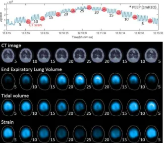
Figure 1: Global impedance (black) curve during PEEP titration in one patient measured with EIT. Regional overdistension (stars) and regional collapse (triangles) were calculated for each PEEP step.
Table 1: Parameters summary of PEEP titration
EIT group Control group
optimal PEEP 18 (3) 15 (4)
PaO2/FiO2 increase 127 (101) 28 (113) increase percentage 125% (92) 26% (112) Increase percentage was referenced to the values before PEEP optimization.
4
Discussion and conclusion
This is a running prospective study using EIT to titrate PEEP in ARDS patients. Based on the preliminary results, PEEP selected in EIT group were higher than that in the control group. This coincided with a previous animal study [7]. The off-line analysis time of the EIT data was ~5 minutes after the end of a PEEP titration, which is acceptable in clinical practice. However, due to the small number of the subjects included in the EIT group, no statistical significance was found. Interquartile ranges were relatively high, which may be due to the mixture of mild moderate and severe ARDS patients in both groups. By further increasing the number of subjects in the EIT group and the retrospective control group, division of the groups according to the severity levels may increase the comparability. Further outcome parameters such as ventilator days, ICU days, weaning successful rate, APACHE II index will be explored.
The preliminary results show that our protocol is feasible and the PEEP titration guided by EIT might lead to a better clinical outcome in ARDS patients.
References
[1] I Frerichs, et al. Thorax, 72: 83-93, 2017 [2] VM Ranieri, et al. JAMA, 307: 2526-33, 2012 [3] MB Amato, et al. N Engl J Med, 372:747-55, 2015
[4] G Franchineau, et al. Am J RespirCrit Care Med, in press 2017 [5] GM Albaiceta, et al. Curr Opin Crit Care, 14:80-6, 2008 [6] E Costa, et al. Intensive Care Med, 35: 1132-37, 2009 [7] GK Wolf, et al. Crit Care Med, 41: 1296-304, 2013
Pulsatile Perfusion Imaging of Premature Neonates using SMS-EIT
Tzu-Jen Kao1, Jonathan Newell2, David Isaacson2, Gary Saulnier2, Bruce Amm1, Greg Boverman1, RakeshSahni3, Marilyn Weindler3, David Chong3, David DiBardino3, David Davenport1, Jeffrey Ashe1 1Diagnostics, Imaging and Biomedical Technologies, GE Global Research Center, Niskayuna, NY 12309, USA, 2Rensselaer Polytechnic Institute, Troy, NY 12180, USA, 3Columbia University Medical Center, New York, NY 10032, USA
Abstract: The aim of this study was to investigate the perfusion signals in premature infants. Five pre-term newborns, (3 males and 2 females, mean (standard deviation, SD) gestational age: 32.6 (0.89) weeks; mean birth weight: 1821 (547.36) g, mean postnatal age: 8.40 (5.03) days), were studied in the Neonatal Intensive Care Unit (NICU) at Columbia University Medical Center. One-hour impedance measurements were made at 18.3 frames/sec with 16-bit precision. Impedance images were reconstructed and displayed in real-time and further analyzed off-line. Frame-by-frame images of pulsatile perfusion were clearly demonstrated without averaging, filtering or contrast agents. The expected phase shift between the pulsatile perfusion waveform in the heart region and in the lung regions was clearly seen. The peak magnitude of the pulsatile signal in the lung region was about half that in the heart region.
1
Introduction
Interest in the clinical use of EIT for monitoring lung function is growing rapidly [1]. But monitoring regional pulmonary perfusion is an unmet clinical need and a technical challenge especially in the neonatal population in which other imaging techniques are rarely used [2].
2
Methods and Results
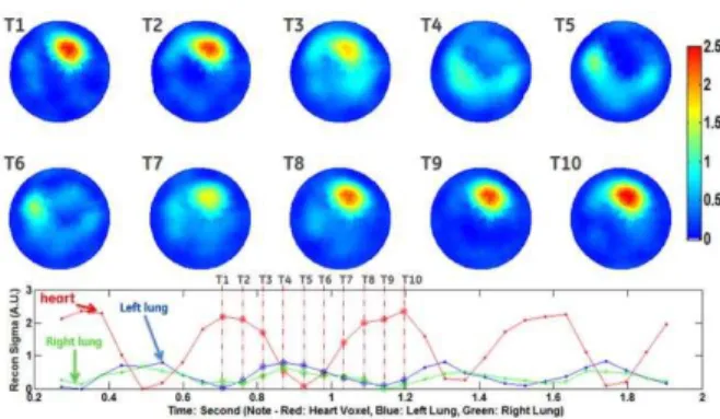
Impedance measurements were made for one hour intervals at 18.3 frames/sec with 16-bit precision using the GE Simultaneous Multi-Source-EIT (SMS-EIT) prototype system [3]. The time-series results in Figures 1 are power waveforms, computed from the first cosine pattern current amplitude multiplied by the real part of the corresponding voltages. Perfusion images were reconstructed during a breathing pause, and regions of interest were selected in the lung and heart fields as shown in Figure 2. Frame-by-frame pulsatile perfusion images were reconstructed in Figure 3 (same scale for different time frames) and Figure 4 (different scale for each subjects).
Figure 1: The power waveforms during the entire 60-minute recordings had significant drift (top). A suitable segment of this signal was selected by hand for detailed analysis (bottom).
Figure 2: Reconstruction mesh, orientation of the impedance images and Regions of Interest (ROI) of the mesh.
Figure 3: Top: Frame by frame reconstructed regional pulsatile perfusion images in the same color scale. The subject’s heart rate is about 140 bpm. Bottom: Red denotes conductivity change in the heart region; blue denotes the left lung region and green denotes the right lung region.
Figure 4:Top: Reconstructed regional pulsatile perfusion image at the end of systole for 5 subjects. Bottom: The comparison of the amplitude of pulsatile perfusion signal in different regions.
3
Conclusions
We have demonstrated the ability of the GE SMS-EIT prototype system to create real-time ventilation and pulsatile perfusion images with impedance data from pre-term neonates. The peak-to-peak magnitude of the pulsatile perfusion signal in the heart region was about 2.2 times that seen in the lung regions, using this 2-D reconstruction algorithm. The phase shift between the perfusion signal in the heart and lungs is clearly observed in Figure 3, and agrees with expectations from normal physiology.
4
Acknowledgement
This research was supported by Grant 1R01HL 109854 from the National Institutes of Health. The content is solely the responsibility of the authors and does not necessarily represent the official views of the National Institutes of Health.
References
[1] A Adler, B Grychtol, R Bayford PhysiolMeas, 36:1067–1074,2015 [2] Caples S M and, Hubmayr R D. 2003 Respiratory monitoring tools
in the intensive care unit Critical Care. 2003; 9:230–235 [3] Kao T-J et al 2014 Real-time 3D electrical impedance imaging for
ventilation and perfusion of the lung with lateral decubitus position Proc. of the IEEE 36th Conf. of the EMBC (Chicago)
Regional Air Distributions in Porcine Lungs using High-performance
Electrical Impedance Tomography System
Geuk Young Jang
2, Hun Wi
2, Young Bok Kim
1, Tong In Oh
1and Eung Je Woo
1 1Department of Medical Engineering, Graduate school, Kyung Hee University, Seoul, Korea, [email protected]2Department of Biomedical Engineering, Graduate school, Kyung Hee University,
![Figure 1: a) Cross section of continuum retina model (reprinted from [2]), b) 32 channel platinum planar electrode array, c) Recon-structed image slice with no noise, d) with uncorrelated system noise.](https://thumb-us.123doks.com/thumbv2/123dok_us/392624.2543649/43.918.465.789.724.920/figure-section-continuum-reprinted-platinum-electrode-structed-uncorrelated.webp)