http://siba-ese.unisalento.it/index.php/ejasa/index e-ISSN: 2070-5948
DOI: 10.1285/i20705948v8n2p246
Factor copulas through a vine structure By Rivieccio
Published: 14 October 2015
This work is copyrighted by Universit`a del Salento, and is licensed un-der aCreative Commons Attribuzione - Non commerciale - Non opere derivate 3.0 Italia License.
For more information see:
DOI: 10.1285/i20705948v8n2p246
Factor copulas through a vine structure
Rivieccio Giorgia
∗Department of Management Studies and Quantitative Methods of Parthenope University Naples, Italy
Published: 14 October 2015
Copula functions have been widely used in actuarial science, finance and econometrics. Though multivariate copulas allow for a flexible specification of the dependence structure of economic variables, they are not particu-larly tempting in high dimensional contexts. A factor model which involves copula functions has already proved to be a powerful tool in credit risk appli-cations.We exploit a recent approach to obtain a factor copula model based on a vine structure, which enables to model the dependence and conditional dependence of variables through a representation of a cascade of arbitrary bi-variate copulas. The contribution of this paper consists into applying the vine copula model in order to derive a non linear three-factor model. In particu-lar, we draw the three-factor model of Fama and French (1992). According to the Inference for Margins (IFM) method, we have computed, separately, the margins and the copula parameters via maximum likelihood estimation. Finally, tail dependence measures are given for the implied estimated copula. keywords: Factor copula model, Vines, Tail dependence, Tail density func-tions.
1 Introduction
The factor approach is a powerful tool in market and credit risk modelling, e.g. for the pricing of CDO, due to its capability in describing, in a both flexible and tractable way, the joint default for a large number of names. One of the most prominent theoretical contributions proposed in literature is the three-factor model of Fama and French (1992), an extension of the well-known Capital Asset Pricing Model (CAPM) (Lintner, 1965; Sharpe, 1964). According to this model, the cross-section of expected stock returns can
∗
c
Universit`a del Salento ISSN: 2070-5948
be explained along a linear three-factor model composed of three common factors: a broad market premium, the spread between small and big market capitalization stocks, and the spread between value and growth stocks.
In particular, the size factor rose from a work of Banz (1981), who verified a negative relationship between average return and firm size. The role of the third factor in ex-plaining the cross-section of average returns was documented by Chan et al. (1991) in the Japanese market.
The factor models proposed in theoretical and empirical applications are often embed-ded into a stochastic correlations framework, implying marginal and joint normality of the stocks and factor returns and of the idiosyncratic cross-sectionally and serially inde-pendent error terms. Moreover, the classical factor models assume the independence of common factor returns but Oh and Patton (2011) have already dropped this assumption. It is widely recognized the evidence of skewness and time conditioning in the univariate behavior of stock returns and, overall, in their whole and tail dependence structure, see e.g., Campbell et al. (2002), Dias and Embrechts (2010), Engle (2002), Longin and Solnik (2001), Patton (2006), to name just a few. Furthermore, Richardson and Smith (1993) show the departure from normality of the asset returns and CAPM residuals. Finally, Chollete and Ning (2010) find evidence of joint tail dependence in several US risk factors.
In order to exploit the cross-section of expected stock returns in non linear way, possibly asymmetrical, a factor approach which involves copula functions is proposed.
A factor copula model allows for computational efficiency, overall in high dimensional contexts, and a flexible specification of the dependence structure, not limited to inde-pendence or linear deinde-pendence.
Introduced by Vasicek (1987) to evaluate the loan loss distribution, and after applied by Li (2000) to multi-name credit derivatives, in terms of Gaussian factor copula, the model was later generalized by Andersen and Sidenius (2004), Gregory and Laurent (2005), Mc-Neil et al. (2005) and van der Voort (2005), which introduced non linear versions. Other extensions include Hull and White (2010), which proposed a two-parameter version of their ”implied copula” model (Hull and White, 2004, 2006). Many of these models are based on simulation or calibration techniques and are not directed to the estimation of copula parameters. Besides, the extension of copula in a multivariate framework requires additional assumptions and it is not an easy task (see Oh and Patton, 2011).
Then, a flexible approach to obtain multivariate copulas can be represented by vines (Bedford and Cooke, 2001), based on the factorization of the multivariate copula den-sity in terms of bivariate linking copulas and lower-dimensional margins. Vines were proposed at first by Joe (1996), as Pair Copula Construction (PCC), later discussed by Bedford and Cooke (2001; 2002), which introduced a graphical representation denoted as regular ”vine”, and by Kurowicka and Cooke (2004; 2006) which defined two partic-ular classes of vine calling them D-vine and C-vine and, finally, developed by Aas et al. (2006) and Aas and Berg (2009), which described statistical inference techniques. In the light of these reasons, adopting a vine structure to draw a multivariate factor copula model allows to:
- depart from linear dependence and gaussian distribution, both via more general marginal distributions and in the dependence structure;
- estimate the copula parameters in a computationally feasible way for high-dimensional continuous variables;
- obtain a flexible specification due to a free selection of copulas involved at various levels of the path-structure from any class and without restrictions on parameters, implying a better description of the joint behavior of the data with different tail dependencies, possibly asymmetric;
- verify the presence of independence between common factors and among variables conditionally on common factors, hypothesized by the classical factor copula ap-proaches.
Brechmann and Czado (2011), Heinen and Valdesogo (2009; 2011) have applied a vine copula model in order to obtain a non linear version of the CAPM, considering an ex-tension which includes the sector effects.
Our proposal is to apply the three-factor model of Fama and French (1992) employing a vine copula structure, with GARCH models for margins. It is the first time that a non linear factor model which involves more than one factor is built in this way. According to the Inference for Margins (IFM) method, we have estimated, separately, the margins and the copula parameters via maximum likelihood estimation. In the first, GARCH models for margins are applied and then, given the conditional independence of the transformed standardized residuals with respect to common factors, vine copulas are estimated, providing the parameters of an implied copula for the asset returns. Finally we have computed tail dependence measures for the ”implied copula” obtained.
The paper is organized as follows. In Section 2 an overview of the three-factor model of Fama and French (1992) is given. Section 3 deals with a theoretical specification of the existing factor copula models. Section 4 describes basic concepts of vine copulas and their use in the factor approach. Section 5 reviews tail dependence measures of vine copulas. Section 6 provides empirical results of the analysis applied to the industry portfolio co-movements conditioned on three common factors. In Section 7, outlook and concluding remarks close.
2 One-factor copula model
In this section a brief review of the three-factor model of Fama and French (1992) is given. The three-factor model was proposed in order to capture the pattern in U.S. average returns associated with size and value versus growth. The Fama and French factors are constructed using the 6 value-weight portfolios from the intersection of two sizes (expressed by Market Equity - ME) and three Book-to-Market Equity (expressed as ratio of Book Equity and Market Equity - BE/ME).
SmBt the average return on the three Small minus the three Big portfolios andHmLt
the average return on the two High BE/ME (value) minus the two Low BE/ME (growth) portfolios, then the three-factor model is given by
Rit−RF t=α+βi[RM t−RF t] +ςiSmBt+γiHmLt+εit
where the left side of the equation denotes the excess of portfolio returns with respect to the risk free asset return, βi is the systematic risk for the portfolio i, εit represents
the idiosyncratic error term for the portfolio i at time t,α is a constant coefficient and, finally, ςi γi are factor loadings for portfolio i.
Although the three-factor model explains the cross-section of expected values in stock returns better than the one-factor model, we need a more general model which goes beyond linear dependence, gaussian distribution, both in the margins and in the depen-dence structure, and orthogonal common factors. In this way, copula functions can be a useful tool to specify a non linear three-factor model.
The factor models postulate that a limited number of common factors suffices to com-pletely explain the dependence structure of the system (see Cherubini et al., 2011). The key concept is ”conditional independence”: conditioning on a specific scenario of the common factors, the economic variables are considered independent each-other. Considering a single common factorY, the conditional joint co-movement of nrandom variables Xi is measured by the product of the marginal conditional probabilities of the
variables with respect to the common factor, given by
P(X1≤x1,· · · , Xn≤xn|Y =y) = n
Y
i=1
P(Xi ≤xi|Y =y)
where the unconditional joint distribution is
P(X1 ≤x1,· · ·, Xn≤xn, Y ≤y) = Z 1 0 n Y i=1 P(Xi≤xi |Y =y)dy
LetFX and FY be the continuous marginal cumulative distribution functions (cdf) of a
bivariate copulaC see, e.g., for definition and theory (see, e.g., for definition and theory Cherubini et al., 2004; Joe, 1997; Nelsen, 2006), then each conditional probability is a partial derivative ofC with respect to the conditioning variable or common factor v
P(X≤x|Y =y) = lim 4y→0P(X≤x|y≤Y ≤y+4y) = ∂C(FX(x), v) ∂v v≡FY(y)
Since each joint probability is defined in terms of copula as
P(X ≤x, Y ≤y) =
Z FY(y)
0
∂C(FX(x), w)
and assuming the conditional independence between variables, we obtain P(X1≤x1,· · · , Xn≤xn|Y =y) = n Y i=1 ∂C(FXi(xi), v) ∂v v≡FY(y) (1)
and the joint co-movement in terms of product of conditional copulas with respect to the common factor
P(X1 ≤x1,· · ·, Xn≤xn, Y ≤y) = Z FY(y) 0 n Y i=1 ∂C(FXi(xi), w) ∂w dw
By using different conditional copula pairs, e.g. by means of a vine structure (see Section 3), one can easily get a more flexible joint distribution, especially in high dimensions. Formally, the one-factor copula model follows (Oh and Patton, 2011)
Xi=h(Y, εi) for i= 1,· · · , n
Y ∼FY(θ), εi ∼iid Fε(θ), Y ⊥εi ∀i
[X1,· · ·, Xn]0 ≡X∼Fx=C(G1(θ),· · ·, Gn(θ);θ)
where the implied copula C(θ) has an unknown form. This generalization reveals that this structure nests a variety of well-known copulas in the literature, see for instance table 1 (see Oh and Patton, 2011). The copula structure involved is too linked to the h
function choice. Adopting a vine structure allows for a flexible choice of h for eachXi.
Our goal is to apply the three-factor model of Fama and French (1992) by means of vine copulas. In general, assumingk common factors denoted asYK = [Y1, ..., Yk]0, we get
Xi=h(YK, εi)
YK ∼FY =C(FY1,· · ·, FYk), εi∼iid Fε, Yk⊥εi ∀i, k (2)
whereC is the copula which allows for the dependence between marginsF.
3 Pair-Copula Constructions (PCC) and vines
Vines are graphical representations of the Pair-Copula Constructions (PCC) which are based on the decomposition of a multivariate density into a cascade of bivariate con-ditional and unconcon-ditional copula densities. Their simple construction, based on pair-copulas as building blocks of the structure, combined to high flexibility, due to the free choice of each pair-copula type from any class and without restrictions on parameters, allows easily to derive higher-dimensional copulas. Let X = (X1, ..., Xn) a vector of n
random variables with marginal densitiesfi(xi), joint cdfF(.) and marginal cdf0sFi(xi),
then the factorization of the joint density f(.) is obtained as
f(x1, . . . , xn) = f(xn|x1, . . . , xn−1)·f(x1, . . . , xn−1) = n Y t=2 f(xt|x1, . . . , xt−1)·f1(x1) (3)
By applying Sklar0s theorem (1959), we get the relationship among an n-dimensional joint density and the copula and marginal densities as
f(x1, . . . , xn) =c1,...,n(F1(x1), . . . , Fn(xn))· n
Y
t=1
ft(xt) (4)
This relationship allows to achieve a PCC decomposition of an n-dimensional density function.
Consideringn= 3 random variables with absolutely continuous joint and marginal cdf0s, then, a possible decomposition of the joint densityf(.) is
f(x1, x2, x3) =f(x3|x1, x2)·f(x2|x1)·f1(x1) (5) where f(x3|x1, x2) =c1,3|2(F(x1|x2), F(x3|x2))·f(x3|x2) (6) and f(xi|xi−1) = f(xi−1, xi)/fi−1(xi−1) = ci−1,i(Fi−1(xi−1), Fi(xi))·fi(xi), i= 2,3 (7) since from (4) f(xi−1, xi) =ci−1,i(Fi−1(xi−1), Fi(xi))fi−1(xi−1)fi(xi), i= 2,3
By replacing the conditional density term in (5) with (6) and (7), the final decomposition of a 3-dimensional PCC can be expressed as
f(x1, x2, x3) = c1,3|2(F(x1|x2), F(x3|x2))·c1,2(F1(x1), F2(x2))·
c2,3(F2(x2), F3(x3))·f1(x1)·f2(x2)·f3(x3) (8)
wherec1,2 and c2,3 are the baseline copulas and c1,3|2 is the conditional copula.
Since factor models assume the conditional independence of variables (see eq. 1) given common factor(s), it results that c1,3|2 in (8) should be equal to one. The conditional
distribution functions, which appear in (8), are obtained as
F(x1|x2) = ∂C1,2(F1(x1), F2(x2)) ∂F2(x2) and F(x3|x2) = ∂C2,3(F2(x2), F3(x3)) ∂F2(x2)
Due to many possible combinations of pair copula decomposition, Bedford and Cooke (2001) introduced a graphical model, denotes as regular vine, in order to organize and visualize them, with the following characteristics:
- an n-dimensional vine is represented by n−1 trees; - j−th tree has (n+ 1−j) nodes and (n−j) edges;
- each edge corresponds to a pair-copula density; - edges in j−th tree become nodes in (j+ 1)−th tree;
- two nodes in (j+ 1)−th tree are joined by an edge only if the corresponding edges inj−th tree share a node;
- the complete decomposition is defined by the n(n−1)/2 edges and the marginal densities.
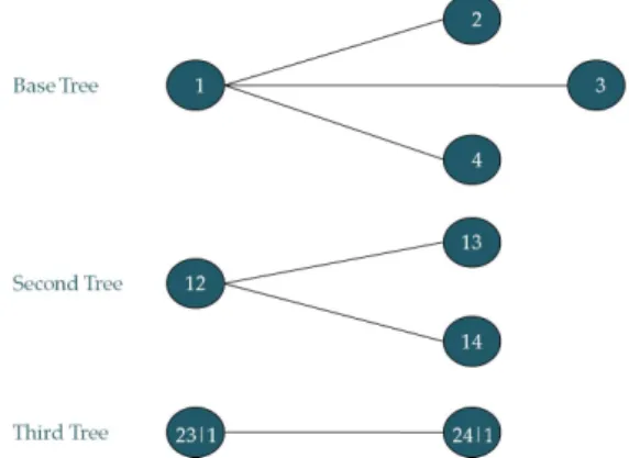
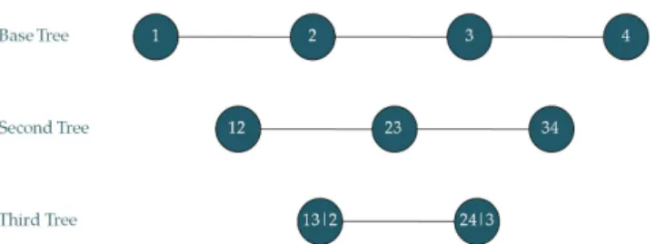
Kurowicka and Cooke (2004) defined two particular classes of regular vine:
- ”C-vine” (Canonical vine) (fig. 1) for which each tree has a unique node that is connected ton−j edges;
- ”D-vine” (fig. 2) for which no node in any tree is connected to more than two edges.
Figure 1 about here Figure 2 about here
Here we are interested in the C-vine structure, based on the specification of a conditioning pilot variable at each level of the construction, characterized by the highest dependence with remaining variables. The density function of a C-vine is expressed as
f(x1, . . . , xn) = n−1 Y j=1 n−j Y i=1 cj,j+i|1,...,j−1(F(xj|x1,...,j−1), F(xj+i|x1,...,j−1)) · n Y k=1 fk(xk). (9)
The conditional distribution functions,F(.|.), which appear in (9), are computed using the following expression (see Joe, 1996)
F(x|v) = ∂Cx,vj|v−j(F(x|v−j), F(vj|v−j))
∂F(vj|v−j)
∀j (10)
where v−j denotes the vector v excluding the component vj. The equation (9) shows
that multivariate copulas can be obtained as product of iteratively conditioned bivariate copulas, where cj,j+l−1 denotes the baseline copula and cj,j+l|j+l−1 is the conditional
copula (forj= 1, ..., n−1 andl= 2, ..., n).
In general, for any vector v−j,x and vj are conditionally independent given v−j if and
only if
cx,vj|v−j(F(x|v−j), F(vj|v−j)) =1 (11) When (11) is verified, v−j is a vector of common factor(s) able to explain the cross
co-movements of the random variablesx and vj (see Granger et al., 2006).
Our goal is to apply the three-factor model of Fama and French (1992) by means of vine copulas, verifying also the presence of a remaining dependence between common factors and among variables conditionally on common factors.
4 Tail dependence of vine copulas
Tail dependence is a useful copula-based measure which defines the relationship in ex-treme values of variables.
This measure of concordance between less probable values is different for each family of copulas since, while it exists for some of them, in a symmetric or asymmetric way, there are families that cannot allow tail dependence.
Joe (1997) and Joe et al. (2010) showed that vine copulas can have a flexible range of bivariate lower and upper tail dependence functions when asymmetric bivariate copulas with upper/lower tail dependence are used in the first level of vine.
Assuming that the bivariate linking copulas have continuous second-order partial deriva-tives, then a vine copula is tail dependent if all the bivariate baseline (base tree) linking copulas are tail dependent. If some baseline copulas are tail independent, then the vine copula is tail independent. Some margins of the vine, however, might still be tail dependent (Joe et al., 2010; Li and Wu, 2011).
The lower and upper tail dependence functions, denoted as bL(.;C) and bU(.;C) are defined as (Joe et al., 2010)
bL(w;C) := lim u→0+ C(uwi,1≤i≤n) u , ∀w= (w1, . . . , wn)∈R n + and bU(w;C) := lim u→0+ ¯ C(1−uwi,1≤i≤n) u , ∀w= (w1, . . . , wn)∈R n +
where C is an n−dimensional copula function and ¯C is its joint survival function. Since a vine copula is expressed in terms of bivariate copula densities, its tail dependence can be derived from tail density approach (Li and Wu, 2011).
LetDwdenote then-order partial differentiation operator with respect to w=(w1,· · · , wn),
then the lower and upper tail density functions are, respectively,
δL(w;C) := lim u→0+ DwC(uwi,1≤i≤n) u = limu→0+u n−1c(uw i,1≤i≤n) = ∂ nbL(w;C) ∂w1,· · · , ∂wn , (12) and δU(w;C) := lim u→0+ DwC¯(1−uwi,1≤i≤n) u = limu→0+u n−1c(1−uw i,1≤i≤n) = ∂ nbU(w;C) ∂w1,· · ·, ∂wn . (13)
Then, in order to obtain the tail density functions, we need to estimate the conditional tail dependence functions.
copula (survival joint function), then the conditional lower and upper tail dependence functions, denoted astL
S1|S2 and t
U
S1|S2, are given by (see Joe et al., 2010)
tLS1|S2(wS1|wS2) = lim u→0+CS1|S2(uwi, i∈S1|uwj, j∈S2) and tUS1|S 2(wS1|wS2) = lim u→0+ ¯ CS1|S2(1−uwi, i∈S1|1−uwj, j∈S2).
LetS0 = (2, .., n−1) be a subset ofS = (1, .., n), then by applying the recursive formulas to build the vine copula structure and assuming that all bivariate baseline linking copulas have lower tail dependence, Li and Wu (2011) proved that
δLS(wS) δL S0(wS0) =c1n(t1|S0(w1|wS0), tn|S0(wn|wS0))δ L 1∪S0(w) δL S0(wS0) δLn∪S0(w) δL S0(wS0) (14)
remarking that fori /∈S0 and 1≤i≤n−lat each l level of the vine (2≤l≤n−1)
δLi|S0(wi|wS0) = ∂ ∂wi tLi|S0(wi|wS0) := δ{Li}∪S0(w{i}∪S0) δL S0(wS0) (15) and δ{L1,n}|S0(w1, wn|wS0) = ∂ 2 ∂w1∂wn tL{1,n}|S0(w1, wn|w{1,n}∪S0) := δ L {1,n}∪S0(w{1,n}∪S0) δL S0(wS0) (16) The expression of the lower tail density of the 3-dimensional vine is:
δ123L (w1, w2, w3) = δ12(w1, w2)·δ23(w2, w3)· c13|2(tL1|2(w1|w2), tL3|2(w3|w2)) (17) wheretLi|2(wi|w2) = R1 0 δ L i2(vi, w2)dvi (i= 1,3).
In high dimensional contexts, in contrast with Joe et al. (2010), the recursion involves only univariate integrals ofn-variate tail densities.
Similar results are obtained for the upper tail density function (see for more details, Li and Wu, 2011).
Note that the expression (14) can be used to show how tail dependence of a vine depends on its bivariate baseline linking copulas.
The existence of tail dependence for all bivariate margins of the vine copulas is guaran-teed by the presence of tail dependence only for the baseline copulas in level 1 and it is not necessary for the conditional bivariate copulas inn−1 levels (as stated in Joe et al., 2010).
at n−1 level of tree (11), according to the hypothesis of conditional independence of portfolio returns of factor models. In particular, Aas et al. (2006) recommend to trun-cate the construction of vine copulas, allowing for product copulas, C⊥, at k level of the structure when the approximation error (measured as difference between conditional density and one, for independence conditional density) is lower than a given threshold. Brechmann et al. (2012) use independence copulas (C⊥) at the k−th tree of the vine. They choose the truncation levelkcomparing the AIC and BIC values of two consecutive models (Ti andTi+1) and the smaller model (Ti) is selected if the latter does not provide
a significant gain in the model fit.
Another way to streamline the vine structure consists in a simplification technique, which allows to capture the residual dependence of asset returns conditioned on common fac-tors. Simplification occurs replacing the remaining pair copulas atklevel of the structure with a gaussian multivariate copula (as in Heinen and Valdesogo, 2009) or with gaussian bivariate copulas (see Brechmann and Czado, 2011).
5 Empirical results
Object of the analysis is the industry equity returns co-movements conditioned on Fama and French three common factors: excess of market return (M kt), SmB andHmL. We have selected five industry portfolio daily returns (January 3rd 2006 - December 30th 2011) provided by Fama and French data library. We report the SIC codes of each variable used afterward:
1. Cnsmr ⇒ Consumer Durables and NonDurables, Wholesale, Retail, and Some Services (Laundries, Repair Shops)
2. M anuf ⇒Manufacturing, Energy, and Utilities
3. HiT ec⇒ Business Equipment, Telephone and Television Transmission 4. Hlth⇒ Healthcare, Medical Equipment, and Drugs
5. Other ⇒ Mines, Constr, BldMt, Trans, Hotels, Bus Serv, Entertainment and Finance.
Although a linear factor model is a good approximation of joint co-movements, it results that the variable HmL is not always significant (in particular, forM anuf, HiT ec and
Hlth). Besides, there is evidence of non gaussian and autocorrelated residuals from all linear regression models, also for the common factors, which are not normally distributed and independent each other.
The estimation of the vine copula parameters can be carried out through a two-step method, defined Inference For Margins (IFM), which computes, separately, the marginal and the copula parameters. In the former, to take into account the conditional depen-dence of variables, GARCH models have been applied to shape the marginal behav-ior of each stock portfolio and factor returns. It results that all variables follow a
which are GJ R−GARCH(1,1) distributed with t-errors. Then, after transforming the standardized residuals into uniform margins, by applying the empirical distribution functions, the bivariate copula parameters are estimated through the maximization of the C-vine log-likelihood. At each step, the estimated parameters became the starting values to the full model estimation.
For eachndimensional random vector of variables, there are n!/2 differentC-vines with
n(n−1)/2 pair copulas (see Aas and Berg, 2009). In order to choose the best permu-tation for theC-vine factorization, it is useful to compute the Kendall0s tau coefficient values for all bivariate pairs, selecting the most dependent pair of assets which become copula-nodes for each tree level (as stated in Aas and Berg, 2009).
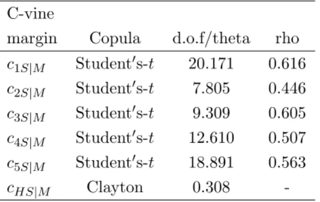
Besides, C-vines are based on the specification of a conditioning pilot variable at each tree level, which maximizes the sum of the absolute Kendalls tau values1. According to the factor approach, in the base tree the pilot variable is M kt, while in the second tree isSmB(see table 2). In order to select the appropriate family for each bivariate copula, we propose a sequential estimation procedure, described in Aas et al. (2006), choosing, at first, the parametric copula with the best fit to the data for each pair of margins and, then, maximizing the full log-likelihood by means of the parameters obtained from the stepwise procedure as starting values. Starting values of the bivariate copula parameters may be determined as follows (as in Aas et al., 2006):
1. Choose the copula types to use in the base tree by plotting the original data and by applying a Goodness-of-Fit (GoF) test, after estimating the parameters of candidate copulas.
2. Generate the observations for the second tree as conditional distribution functions of the original data using the estimated copula parameters.
3. Determine which copula types to use in the second tree in the same way as in the base tree.
4. Proceed iterating.
The main characteristic of a vine copula is the free specification ofn(n−1)/2 bivariate copulas which do not have to belong to the same family and can have a flexible range of bivariate upper/lower tail dependence parameters, different for each margin pair when asymmetric bivariate copulas with upper/lower tail dependence are used in the base tree of the vine (see for more details Joe et al., 2010).
Asymmetric copulas generally involved in the analysis of tail dependence are: the Clay-ton with lower tail dependence, the Gumbel with upper tail dependence,the BB1 and the BB7 (see Joe, 1997) with both tail dependencies.
We have also selected, for sake of comparisons, the Gaussian copula without tail depen-dence (which is the standard market model), the Student0s-t copula with symmetrical tail dependence and the product copula for independence. This last copula is selected according to the bivariate independence test based on Kendall’s tau (Genest and Favre,
1
2007).
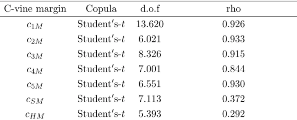
In order to select the copula with the best fit to the data, we have compared, at each tree level, the log-likelihood functions through Akaike Information Criterion (AIC) and the Bayesian Information Criterion (BIC). It results that the Student0s-tcopula is more preferred to other copula functions, this implies the prevalence of a symmetrical tail dependence. Tables from 3 to 9 show copula parameter estimates. We can note a signi-ficative dependence among common factors expressed by the last two copulas, contrary to the assumptions of the linear factor models.
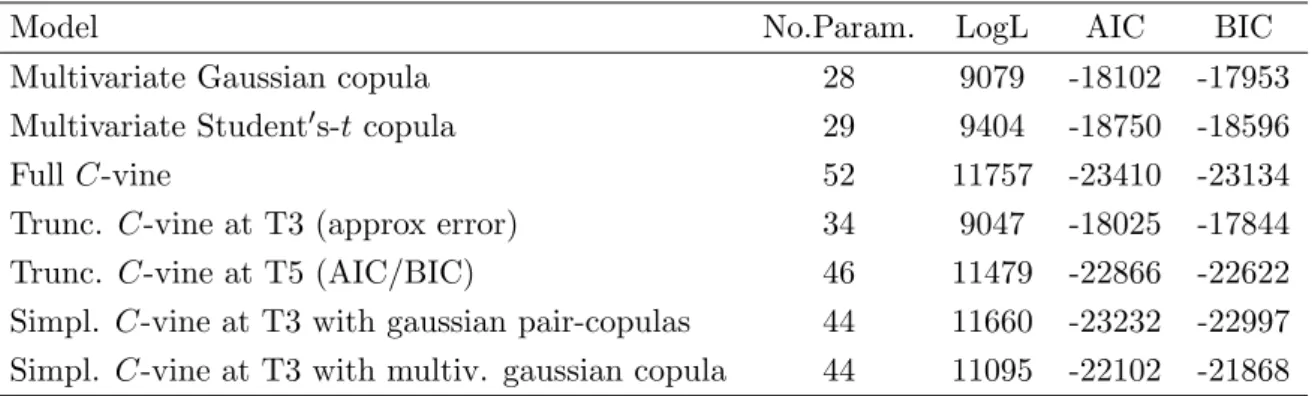
Moreover, we have compared theC-vine factor copula model with other multivariate cop-ulas and the results (table 10) remark the best performance of C-vine, especially over the standard linear gaussian model of Fama and French (1992). Besides, since a vine copula structure can be truncated, according to the hypothesis of conditional indepen-dence of portfolio returns, or simplified, in order to capture the remaining depenindepen-dence of asset returns conditional on common factors, we have computed the maximum likeli-hood copula parameters of the truncated (with an approximation error lower than 0.01) and simplified version of the fullC-vine model. The best alternative to the full C-vine model, in a factor model perspective, is the simplifiedC-vine with gaussian copula pairs (table 10). This implies a conditional dependence which is not accurately captured by the standard factor model.
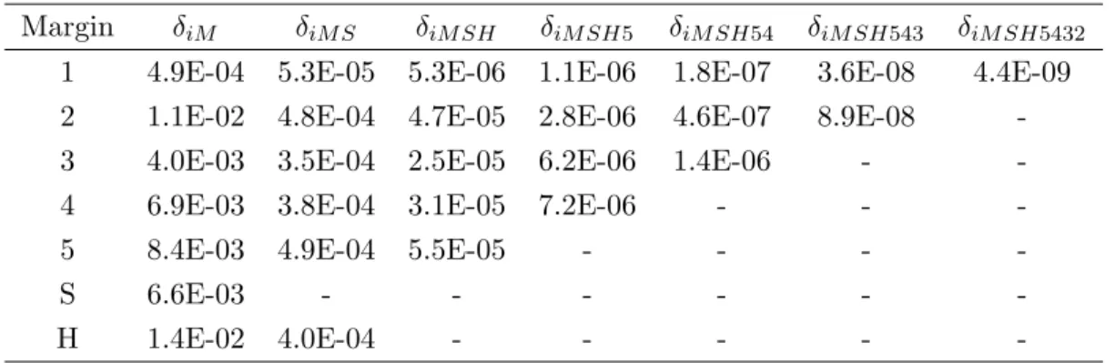
Finally, we provide the tail density functions of fullC-vine model, according to equations (14) - (17), to measure the dependence between extreme realizations of portfolio returns. In table 11 we report the lower tail density functions of all margins which are building blocks of the conditional copulas included in the model. Since all bivariate baselines linking copulas are tail dependent (Student0s-t), also the vine copula is tail dependent, although weakly (see, for the lower tail density,δ12345M SH in table 11).
6 Outlook and Conclusions
In this paper we combine the factor approach with vine copulas in order to obtain the non linear three-factor model of Fama and French (1992). This is the first contribution which draws a three-factor model by use of vine copulas. Second, we provide empirical estimates of tail dependence measures for the vine copulas, based on tail density func-tions, which involve only one-dimensional integrations.
Different reasons have led to develop a three-factor copula model by means of a vine structure. First of all, the need to consider non-linear dependence measures and some alternatives to the elliptical distributions, both in margins and in the joint distributions. Vines allow for a free specification of bivariate copulas involved in the model, which can belong to distinct families with a flexible range of tail dependence parameters, different also for each margin pair. Second, the extension of copulas in multivariate contexts requires additional assumptions and it is not an easy task. The simple structure of vine copulas, based only on bivariate copulas, allows to compute easily, by MLE method, copula parameters for high-dimensional continuous variables. In brief, combining a vine structure with the factor copula approach enables a flexible construction of high
di-mensional, also non elliptical, joint distributions of cross-section of the expected stock returns, able to capture possible asymmetries in tail dependence. The main result of the application is that the vine factor copula model performs better than other multivariate models, also more than the classical linear factor approach. Besides, it emerges the ex-istence of a conditional dependence between variables with respect to common factors in addition to that observed among the common factors.
Future researches will concentrate on some alternative models, which can include: the momentum factor, defined as the amount of acceleration of stocks (see for instance Carhart, 1997), time-varying factors or other common factors resulting from a Principal Component Analysis (PCA) applied to the stock asset returns.
References
Aas, K., Berg, D. (2009). Models for construction of multivariate depen-dence: A comparison study. European Journal of Finance, 15, 639-659. DOI:10.1080/13518470802588767
Aas, K., Czado, C., Frigessi, A., Bakken, H. (2006). Pair-copula constructions of multiple dependence. Insurance: Mathematics & Economics, 44, 182-198.
Andersen, L., Sidenius, J. (2004). Extensions of the Gaussian Copula Model. Journal of Credit Risk, 1, 29–70.
Banz, W. (1981). The relationship between return and market value of common stocks. Journal of Financial Economics, 9, 3–18.
Bedford, T., Cooke, R. M. (2001). Probability density decomposition for conditionally dependent random variables modeled by vines. Annals of Mathematics and Artificial Intelligence, 32, 245-268. DOI:10.1023/A:1016725902970
Bedford, T., Cooke, R. M. (2002). Vines - a new graphical model for dependent random variables. Annals of Statistics, 30, 1031-1068. DOI:10.1214/aos/1031689016
Brechmann, E.C., Czado, C. (2011). Risk management with high-dimensional vine copulas: An analysis of the Euro Stoxx 50. Working paper, Technische Universit¨at M¨unchen.
Brechmann, E.C., Czado, C., Aas, K. (2012). Truncated Regular Vines in High Di-mensions with Applications to Financial Data. Canadian Journal of Statistics, 40, 68–85.
Campbell, R., Koedijk, K., Kofman, P. (2002). Increased correlation in bear markets. Financial Analysts Journal, 58, January-February, 87–94. ISSN: 0015198X
Carhart, M.M. (1997). On persistence in mutual fund performance Journal of Finance, 52, 57–82.
Chan, L.K., Hamao, Y., Lakonishok, J. (1991). Fundamentals and stock returns in Japan. Journal of Finance, 46, 1739–1789.
Cherubini, U., Luciano, E., Vecchiato, W. (2004). Copula Methods in Finance. John Wiley & Sons.
Cherubini, U., Gobbi, F., Mulinacci, S., Romagnoli, S. (2011).Dynamic Copula Methods in Finance. John Wiley & Sons.
Chollete, L., Ning, C. (2010). Asymmetric Dependence in US Financial Risk Factors?, US Working Papers in Economics and Finance, 2/11, University of Stavanger. Dias, A., Embrechts, P. (2010). Modeling exchange rate dependence dynamics at
differ-ent time horizons. Journal of International Money and Finance, 29, 1687–1705. DOI: 10.1016/j.jimonfin.2010.06.004
Engle, R F. (2002). Dynamic conditional correlation: a simple class of multivariate generalized autoregressive conditional heteroscedasticity models. Journal of Business and Economic Statistics, 20, 339–350. DOI:10.1198/073500102288618487
Fama, E.F., French, K.R. (1992). The cross-section of expected stock returns. Journal of Finance, 47, 427-465.
Genest, G., Favre, A. (2007). Everything You Always Wanted to Know about Copula Modeling but Were Afraid to Ask. J. Hydrol. Eng., 12, Special issue: Copulas in Hydrology, 347-368. DOI: 10.1061/(ASCE)1084-0699(2007)12:4(347)
Granger, C.W.J., Ter¨asvirta, T., Patton, A. (2006). Common factors in condi-tional distributions for bivariate time series. Journal of Econometrics, 132, 43-57. DOI:10.1016/j.jeconom.2005.01.022
Gregory, J., Laurent, J.P. (2005). Basket Default Swaps, CDOs and Factor Copulas. Journal of Risk, 7, 8-23.
Heinen, A., Valdesogo, A. (2009). Asymmetric CAPM dependence for large dimensions: the Canonical Vine Autoregressive Model.CORE Discussion Papers 2009069, Univer-sit catholique de Louvain, Center for Operations Research and Econometrics (CORE). Available at http://dx.doi.org/10.2139/ssrn.1297506
Heinen, A., Valdesogo, A. (2011). Dynamic D-vine Model. In: Kurowicka, D., Joe, H. (Eds.). Dependence Modeling: Vine Copula Handbook. World Scientific, 329–353. Hull, J., White, A. (2004). Valuation of a CDO and nth to default CDO without Monte
Carlo Simulation. Journal of Derivatives, 12, 10-23.
Hull, J., White, A. (2006). Valuing Credit Derivatives Using an Implied Copula Ap-proach. Journal of Derivatives, 14 2, 8-28.
Hull, J., White, A. (2010). An improved implied copula model and its application to the valuation of bespoke CDO tranches. Journal of investement management.
Joe, H. (1996). Families of m-variate distributions with given margins and m(m-1)/2 bivariate dependence parameters. In: R¨uschendorf, L., Schweizer, B., Taylor, M.D.(Eds.). Distributions with Fixed Marginals and Related Topics.
Joe, H. (1997). Multivariate Models and Dependence Concepts. Chapman & Hall/CRC, New York.
Joe, H., Li, H., Nikoloulopoulos, A. K. (2010). Tail dependence func-tions and vine copulas. Journal of Multivariate Analysis, 101, 252–270. http://dx.doi.org/10.1016/j.jmva.2009.08.002
depen-dence and applications to financial return data. Computational Statistics and Data Analysis.
Kurowicka, D., Cooke, R. M. (2004). Distribution-free continuous bayesian belief nets. In Fourth International Conference on Mathematical Methods in Reliability Methodology and Practice, Santa Fe, New Mexico.
Kurowicka, D., Cooke, R. M. (2006). Uncertainty Analysis with High Dimensional De-pendence Modelling. Wiley, New York.
Li, D.X. (2000). On Default Correlation: A Copula Approach. Journal of Fixed Income, 9, 43–54.
Li, D.X., Wu, P. (2011). Extremal Dependence of Copulas: A Tail Density Approach. Working Paper.
Lintner, J. (1965). The valuation of risk assets and the selection of risky investments in stock portfolios and capital. Review of Economics and Statistics, 47, 13–37.
Longin, F., Solnik, B. (2001). Extreme correlation of international equity markets. The Journal of Finance, 56, 649–676. DOI: 10.1111/0022-1082.00340.
McNeil, A. J., Frey, R., Embrechts, P. (2005). Quantitative Risk Management.Princeton University Press, New Jersey.
Nelsen, R. B.(2006). An Introduction to Copulas. Springer-Verlag, New York.
Oh, D.H., Patton, A. (2011). Modelling Dependence in High Dimensions with Factor Copulas. Working Paper. Revised April 2012.
Patton, A. (2006). Modelling asymmetric exchange rate dependence. International Economic Review, 47, 527–556. DOI:10.1111/j.1468-2354.2006.00387.x
Richardson, M., Smith, T. (1993). A test for multivariate normality in stock returns. Journal of Business, 66, 2, 295–321.
Sharpe, W.F. (1964). Capital asset prices: a theory of market equilibrium under condi-tions of risk. Journal of Finance, 19, 425–442.
Sklar, A. (1959). Fonctions de r´epartition `a n dimensions et leurs marges. Publ. Inst. Statist. Univ. Paris, 8, 229–231.
Vasicek, O.(1987). The Loan Loss Distribution. Working Paper, KMV.
van der Voort, M. (2005). Factor copulas: totally external defaults. Working Paper, Erasmus University Rotterdam.
Table 1: Example of some copula densities known in a closed form as function of h,
Fy and of F (Oh and Patton, 2011).∗Gamma distribution, ∗∗Inverse Gamma
distribution
Copula h(Y,) FY F
Gaussian Y + N(0, σY2) N(0, σ2) Student0s-t Y1/2 Ig∗∗(v/2, v/2) N(0, σ2) Clayton (1 +/Y)−a Γ∗(a,1) Exp(1) Gumbel −(logY /)a Stable(1/a,1,1,0) Exp(1)
Table 2: Kendall0s Tau Estimates. Mkt=Excess of Market return with respect to risk free rate, SmB=Small minus Big portfolios, HmL=High minus Low portfolios
Portfolio Mkt SmB HmL Cnsmr 0.750 0.409 0.172 Manuf 0.762 0.348 0.195 HiTec 0.730 0.415 0.120 Hlth 0.637 0.393 0.108 Other 0.761 0.392 0.222
Table 3: Copula parameter estimates in the Base Tree
C-vine margin Copula d.o.f rho
c1M Student0s-t 13.620 0.926 c2M Student0s-t 6.021 0.933 c3M Student0s-t 8.326 0.915 c4M Student0s-t 7.001 0.844 c5M Student0s-t 6.551 0.930 cSM Student0s-t 7.113 0.372 cHM Student0s-t 5.393 0.292
Table 4: Copula parameter estimates in the Second Tree C-vine
margin Copula d.o.f/theta rho
c1S|M Student0s-t 20.171 0.616 c2S|M Student0s-t 7.805 0.446 c3S|M Student0s-t 9.309 0.605 c4S|M Student0s-t 12.610 0.507 c5S|M Student0s-t 18.891 0.563 cHS|M Clayton 0.308
-Table 5: Copula parameter estimates in the Third Tree C-vine
margin Copula d.o.f rho
c1H|M S Gaussian - 0.215
c2H|M S Student0s-t 11.668 0.347
c3H|M S Student0s-t 10.982 0.088
c4H|M S Student0s-t 13.295 0.190
c5H|M S Student0s-t 22.931 0.436
Table 6: Copula parameter estimates in the Fourth Tree C-vine
margin Copula d.o.f rho
c15|M SH Student0s-t 14.242 0.423
c25|M SH BB1 0.659 1.033
c35|M SH Student0s-t 25.697 0.566
Table 7: Copula parameter estimates in the Fifth Tree C-vine
margin Copula d.o.f/theta rho
c14|M SH5 Clayton 0.744
-c24|M SH5 Clayton 0.331
-c34|M SH5 Student0s-t 21.705 0.650
Table 8: Copula parameter estimates in the Sixth Tree C-vine
margin Copula d.o.f rho
c13|M SH54 Student0s-t 38.651 0.159
c23|M SH54 Student0s-t 34.939 0.009
Table 9: Copula parameter estimates in the Seventh Tree C-vine
margin Copula d.o.f rho
c12|M SH543 Student0s-t 34.330 0.354
Table 10: Model Comparison
Model No.Param. LogL AIC BIC
Multivariate Gaussian copula 28 9079 -18102 -17953
Multivariate Student0s-tcopula 29 9404 -18750 -18596
FullC-vine 52 11757 -23410 -23134
Trunc. C-vine at T3 (approx error) 34 9047 -18025 -17844 Trunc. C-vine at T5 (AIC/BIC) 46 11479 -22866 -22622 Simpl. C-vine at T3 with gaussian pair-copulas 44 11660 -23232 -22997 Simpl. C-vine at T3 with multiv. gaussian copula 44 11095 -22102 -21868
Table 11: Tail densities of all margins (w= 1)
Margin δiM δiM S δiM SH δiM SH5 δiM SH54 δiM SH543 δiM SH5432
1 4.9E-04 5.3E-05 5.3E-06 1.1E-06 1.8E-07 3.6E-08 4.4E-09 2 1.1E-02 4.8E-04 4.7E-05 2.8E-06 4.6E-07 8.9E-08 -3 4.0E-03 3.5E-04 2.5E-05 6.2E-06 1.4E-06 -
-4 6.9E-03 3.8E-04 3.1E-05 7.2E-06 - -
-5 8.4E-03 4.9E-04 5.5E-05 - - -
-S 6.6E-03 - - -