Working Paper No. 29
Copula bivariate probit models: with an
application to medical expenditures
Rainer Winkelmann
September 2011
University of Zurich
Department of Economics
Working Paper Series
ISSN 1664-7041 (print)
ISSN1664-705X(online)
Copula bivariate probit models: with an
application to medical expenditures
Rainer Winkelmann
∗University of Zurich, CESifo and IZA
July 2011
Abstract
The bivariate probit model is frequently used for estimating the effect of an endogenous binary regressor (the “treatment”) on a binary health outcome variable. This paper discusses simple modifications that maintain the probit assumption for the marginal distributions while introducing non-normal dependence using copulas. In an application of the copula bivariate probit model to the effect of insurance status on the absence of ambulatory health care expen-diture, a model based on the Frank copula outperforms the standard bivariate probit model.
Keywords: Bivariate probit, binary endogenous regressor, Frank copula, Clayton copula.
Running head: Copula bivariate probit models
Word count: 4553
∗Address for correspondence: University of Zurich, Department of Economics, Zurichbergstr. 14, CH-8032 Zurich,
Switzerland, phone: +41 (0)44 634 22 92, fax: +41 (0)44 634 49 96, email: [email protected]. I thank two anonymous referees for very useful comments.
1
Introduction
The bivariate probit model is frequently used in health economics when one wants to estimate the effect of a treatment on a binary health outcome. It arises from a 2-equation structural latent variable framework, where the first equationy1 =1(β0+β1y2+ε1 >0) describes the health outcome variable (y1) as a function of a binary treatment (y2) and latent errorε1, whereas the second equation
y2 =1(π0+π1z+ε2 >0) determines whether or not treatment is received. The model is completed by assuming that the latent errorsε1 andε2have a bivariate standard normal joint distribution with correlationρ. Ifρ= 0, separate estimation of the first structural equation by a simple probit model identifies the structural treatment effect β1. If ρ 6= 0, the treatment is said to be “endogenous”, and joint estimation is required. Recent applications in this journal include Dormont et al. (2009), French and Maclean (2006), Gitto et al. (2006), Latif (2009), MacDonald and Shields (2004), Smith Conway and Kutinova (2006). The bivariate probit model is also discussed in popular textbooks on health econometrics by Jones and O’Donnell (2002) and Jones (2007).
The purpose of this paper is to propose an alternative, general class of structural probit mod-els that allow for correlation between the two latent errors (and hence endogenously determined treatment) without imposing joint normality. A key component of this approach is the concept of a copula (see e.g. Joe, 1997, Nelson, 2007, Trivedi and Zimmer, 2007) which treats the modeling of marginal distributions and of dependence structure as separate tasks. Copulas thereby provide a convenient device for generating a flexible non-normal distribution for the errors. The parameters of the resultingcopula bivariate probit model (CBP) can be estimated by maximum likelihood.
variable models. Lee (1983) uses copulas to generalize the normality assumption that underpins the selectivity model of Heckman (1976). In his case, the structural two equation system consists of a continuous outcome equation and a latent selection equation. Continuous copulas are used to construct the joint distribution of error terms in the two equations. Extensions of this approach were provided by Prieger (2002) and Smith (2003). Smith (2005) derives a copula-based switching regression model, again for a continuous dependent variable. A regression model with binary en-dogenous variable can be obtained as a special case. To the best of my knowledge, the use of copula theory for structural bivariate binary response models has not been considered so far.
I discuss two specific versions of the CBP model, one based on the Frank copula, and one based on the Clayton copula. On one hand, these copulas have been chosen because they are simple and the resulting models require, in contrast to the standard bivariate probit, no numerical integration in order to compute probabilities. On the other hand, the dependence structure they imply departs in interesting ways from that of a bivariate normal distribution. While the conditional expectation function (cef) of the latter is linear, the Frank CBP model has a cef that becomes flat in the tails (signifying mean independence once the conditioning event is sufficiently rare), whereas the Clayton CBP model has an asymmetric cef.
The paper includes a formal Monte Carlo analysis showing that it is possible to empirically discriminate between the different CBP models. Furthermore, using a wrong copula can lead to substantial bias in the estimation of structural parameters. The proposed approach is illustrated in an application to the endogeneity of insurance choice in a model for ambulatory health expenditures, following Deb et al. (2006).
2
Econometric Methods
2.1
Bivariate probit model
The bivariate probit model provides a convenient setting for estimating the effect of an endogenous binary regressor y2 on a binary outcome variable y1. The standard model assumes a constant treatment effect, the presence of exclusion restriction, and the absence of simultaneity. Formally, the structural model consists of two latent equations
y1∗ =xβ+αy2+ε1 (1)
y2∗ =zγ+ε2 (2)
where the stochastic errors that are independent ofxandz but not necessarily independent of each other. Moreover, the observed binary outcomes are
y1 =1(y1∗ >0), y2 =1(y∗2 >0)
where1(·) is the indicator function. The main interest is in the structural treatment parameterα, or the average treatment effect Ex[P(ε1 >−xβ−α)−P(ε1 >−xβ)]. The joint distribution of y1 and y2 (conditional on x and z) has four elements:
P(y1 = 0, y2 = 0|x, z) = P(ε1 ≤ −xβ, ε2 ≤ −zγ) (3)
P(y1 = 1, y2 = 0|x, z) = P(ε1 >−xβ, ε2 ≤ −zγ) (4)
P(y1 = 1, y2 = 1|x, z) = P(ε1 >−xβ−α, ε2 >−zγ) (6)
This distribution is fully determined once the joint distribution of ε1 and ε2 is known. In the bivariate probit model, it is assumed that ε1 and ε2 have joint distribution function F(ε1, ε2) = Φ2(ε1, ε2, ρ) where Φ2 denotes the cumulative density function of the bivariate standard normal distribution, and ρ is the coefficient of correlation. In this case, the joint probability function
f(y1, y2|x, z) can be written compactly as
f(y1, y2|x, z) = Φ2[s1(xβ+αy2), s2(zγ), s1s2ρ] (7)
wheresj = 2yj −1,j = 1,2.
It is important to understand that the thus defined bivariate probit model introduces two sources of dependence between y1 and y2, related to the parameters α and ρ, respectively. While the joint model simplifies to two univariate probit equations under independence of the structural errors (ρ = 0), this does not mean that y1 and y2 are independent in this case. The reason is that the first probit equation of the recursive base model gives the probability of y1 conditional on y2. Therefore, full independence ofy1 and y2 requires ρ= 0 and α = 0. The CBP model developed in this paper uses copulas to model dependence between the structural errors. It does not model the dependence between the two binary outcomes directly, although dependence between the structural errors obviously affects that dependence.
2.2
Clayton and Frank copulas and their properties
Any joint distribution function has a copula representation in which dependence and marginals are separately specified, or “uncoupled”. Copulas are thus building blocks for multivariate distributions
that preserve the probit assumption for the two equations (1) and (2) but do not impose joint normality. In particular, one can recur to well known parametric classes of copula functions that allow for different kinds of dependence and often have quite simple functional forms.
Formally, a copula is a multivariate joint distribution function defined on the n-dimensional unit cube [0,1] such that every marginal distribution is uniform on the interval [0,1] (see, e.g., Nelson, 2006). For example, for n = 2, we can write C(u, v) = P(U ≤ u, V ≤ v), with marginal distributions given by P(U ≤ u, V ≤ 1) = C(u,1) and P(U ≤ 1, V ≤ v) = C(1, v), respectively. The normal, or Gaussian, copula, again forn= 2, is
P(U ≤u, V ≤v) = C(u, v) = Φ2(Φ−1(u),Φ−1(v);θ) (8)
where θ is the coefficient of correlation. Apart from the Gaussian copula and the independence copulaC(u, v) =uv, I consider in this paper two further copulas, the Clayton copula
C(u, v) = (u−θ+v−θ−1)−1/θ (9)
and the Frank copula
C(u, v) =−θ−1log ( 1 + (e −θu−1)(e−θv −1) (e−θ−1) ) (10)
It is easy to verify that all four copulas (Gaussian, independence, Clayton, Frank) have uniform marginal distributions, as C(u,1) = uand C(1, v) =v.
The significance of copulas in the present context lies in the fact that by way of transformation, they can be used to generate joint distribution functions for the two structural errors in the bivariate probit model,ε1 andε2, keeping the normal marginals but without assuming full bivariate normality.
Letu= Φ(ε1) and v = Φ(ε2). Then F(ε1, ε2) =C(Φ(ε1),Φ(ε2)) is a joint distribution function for
ε1 and ε2 with marginal distributions that are standard normal.
For example, the normal copula recovers the standard bivariate probit model, since
F(ε1, ε2) = Φ2[Φ−1(Φ(ε1)),Φ−1(Φ(ε2))] = Φ2(ε1, ε2)
whereas under the Clayton assumption
F(ε1, ε2) = (Φ(ε1)−θ+ Φ(ε2)−θ−1)−1/θ
In order to compare the differences in the dependence structure implied by the Frank and Clayton copulas to that of the bivariate normal distribution, correlation is not a good indicator. First, it detects only linear dependence, whereas dependence in copulas is non-linear in general. Second, and relatedly, it is not invariant to transformation of the marginal distributions. As a consequence, other measures of dependence have been suggested. A common one is Kendall’s τ, a measure of the degree of concordance. Imagine drawing two random pairs (U1, V1) and (U2, V2) from the joint distribution ofU and V. Then τ is defined as
τ =P[(U1 −U2)(V1 −V2)>0]−P[(U1−U2)(V1−V2)<0]
τ can vary between -1 and 1. It is zero if U and V are independent. Not all copulas cover the full spectrum of possible τ’s. If they do so, they are called comprehensive. The normal and Frank copulas are comprehensive, whereas the Clayton copula (9) is not, the reason being that it only captures positive dependence. It is “half comprehensive”, however, sinceτ can take any value between 0 and 1. Of course, one can always reflect a Clayton copula, modeling the relationship
betweenU and −V instead, in which case the dependence is strictly negative, with τ’s between -1 and 0.
− − − − − − − − − Figure 1 about here − − − − − − − − −
Additional insight into the nature of dependence implied by these copula models can be obtained from their conditional expectation functions. The cef of the bivariate normal distribution is linear, with E(ε2|ε1) = ρε1. For the Clayton and Frank copula, simple expressions for the conditional expectations are not available, but it is straightforward to obtain them by way of simulation. Figures 1 and 2 show a sample of 500 draws from the Frank and Clayton copulas, with standard normal marginals, for θ = 3.3 and θ = 1, respectively. Also shown are the cefs (obtained from a nonparametric regression) as well as the linear regression line.
− − − − − − − − − Figure 2 about here − − − − − − − − −
The Frank copula is symmetric. Its cef is near linear in the center but flattens out in the tails. This is an interesting feature that can be of value in applications to sample selection models where the linearity of the cef of the bivariate normal distribution lacks plausibility when selection probabilities are very small. The Clayton copula looks quite different. It is not symmetric, and the cef shows much stronger dependence in the left tail of the distribution than in the right. Again, this is a distinctive feature that may bea-priori desirable in some applications.
2.3
Copula bivariate probit model
The generic probability expressions for the bivariate probit model were given in equations (3) – (6). Under a copula representation with probit marginals, these expressions can be written as
P(y1 = 0, y2 = 0) =C[Φ(−xβ),Φ(−zγ)] (11)
P(y1 = 1, y2 = 0) =C[1,Φ(−zγ)]−C[Φ(−xβ),Φ(−zγ)] (12)
P(y1 = 0, y2 = 1) =C[Φ(−xβ−α),1]−C[Φ(−xβ),Φ(−zγ)] (13)
P(y1 = 1, y2 = 1) = 1−C[Φ(−xβ−α),1]−C[1,Φ(−zγ)] +C[Φ(−xβ−α),Φ(−zγ)] (14)
The joint probabilities of the CBP model depend on the selected copula as well as on four param-eters, ξ = (β, γ, α, θ), where θ is the dependence parameter of the copula function. If the true copula is assumed to belong to a parametric family C = {Cξ, ξ ∈ Ξ}, a consistent and asymp-totically normally distributed estimator of the parameter ξ can be obtained through maximum likelihood. Assuming an independent sample ofn observations (yi1, yi2, xi, zi), the likelihood func-tion L(ξ;y1, y2, x, z) is proportional to n Y i=1 P(yi1 = 1, yi2 = 1)yi1yi2 ×P(yi1 = 1, yi2 = 0)yi1(1−yi2) ×P(yi1 = 0, yi2 = 1)(1−yi1)yi2 ×P(yi1 = 0, yi2 = 0)(1−yi1)(1−yi2)
Numerical optimization methods can be used to maximize the log-likelihood function. These can employ analytical first derivatives that have a relatively tractable form. For example,
∂P(y1 = 0, y2 = 0|ξ)
where cu = ∂C(u, v)/∂u. A formal requirement for identification is that there is at least one exogenous regressor with a non-zero coefficient, i.e.,β 6= 0 or γ 6= 0 (Wilde, 2000). As long as the model is correctly specified, the maximum likelihood estimator has the usual asymptotic properties. It is useful to think of these estimators as providing best approximations to an unknown true model, in a quasi-likelihood sense (White, 1982), and a robust covariance estimator should be used.
3
Results
3.1
Simulation Study
To learn about the behavior and performance of the CBP model under various data generating processes (DGP), I report results for a simulation experiment carried out in order to evaluate the bias and accuracy of the estimators as well as model selection. The DGP is a simple recursive model for two binary dependent variables with probit margins:
y1 =1(β0+β1x+αy2+ε1 >0)
y2 =1(γ0+γ1z+ε2 >0)
where (β0, β1, γ0, γ1, α) = (0.5,−0.5,0,1,0.5). In all cases x and z are iid Gaussian with mean zero and standard deviation 1.
The stochastic errors ε1 and ε2 are generated from three alternative copula models:
• Normal copula with ρ= 0.5
• Clayton copula with θ = 1
The dependence parameters have been chosen to yield the same value for τ in all three cases, namely 0.33. The marginal distributions of the stochastic errors ε1 and ε2 are standard normal. Given the parameter values and the distribution ofx and z, the mean of y1 is approximately 73%, while the mean of y2 is approximately 50%. The simulations are conducted for three sample sizes
n= 500,1000,5000, and run for r= 5000 replications each.
− − − − − − − − − Table I about here − − − − − − − − −
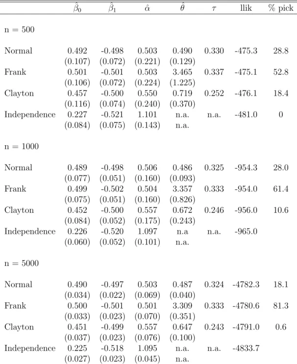
The results are shown in Table I (Normal DGP), Table II (Frank DGP) and Table III (Clayton DGP). When looking at the results, there are two key questions of interest. First, what are the biases that result from estimating the wrong model?; and second, do tests and model selection criteria reveal the right model? The Gaussian, Clayton and Frank copulas nest the independence copula, so a test for independence can be based on the likelihood ratio test statistic. In the case of the Clayton copula, a small adjustment is needed, as θ sits at the boundary of the parameter space under the null hypothesis. Chernoff (1954) shows for this case, that the distribution of the likelihood ratio statistic under the null is mixed discrete and continuous, with probability mass of 0.5 at 0 and half a χ2(1) distribution for positive values. To select among the three dependence copulas (which are non-nested), application of information criteria reduce to simple log-likelihood comparisons, as the number of parameters is the same in the three models.
From Table I, we see that the parameter of the exogenous regressor β1 (the true value is -0.5) is estimated well regardless of model and sample size. However, the parameter of the endogenous regressorαis subject to bias in the misspecified models. The bias is very large for the independence model, where it amounts to over 100 % but there is also substantial bias for the Clayton copula. Forn = 500, for instance, the Clayton mean is 0.549, compared to the true value of 0.5. The bias does not vanish as the sample size increases.
The average likelihood ratio test statistic for the independence model against the normal model is 11.6 for n = 500, increasing to 107.4 for n = 5000. While the simulation results show that the copula models do well in detecting dependence, they also show that larger samples are needed to reliably discriminate between the three copulas with dependence. For example, while the correctly specified normal copula model has the highest average log-likelihood even ifnis only 500, the Frank copula model is picked instead in a substantial proportion of instances (33.6%) when model selection is based on the highest log-likelihood value. The situation improves considerably when the sample size is increased to 5000. Now, the correct model is picked in 80% of all simulation runs.
− − − − − − − − − Table II about here − − − − − − − − −
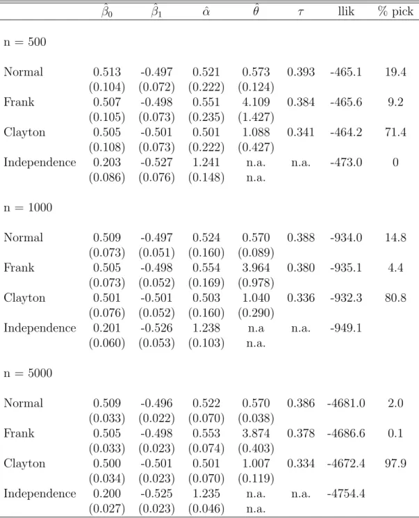
These qualitative conclusions are largely confirmed by the other two DGPs in Tables II and III. In Table II, data are generated from a Frank copula with dependence parameter θ = 3.3. Again, the correct model estimates the true parameter values accurately on average, even for the smallest sample size, whereas a misspecified model tends to overestimate the structural parameterα. There
is one exception, though, since the normal copula appears to provide an unbiased estimator as well, indicating a certain degree of robustness. Also in terms of log-likelihood value, Frank and normal copula are closest to each other, which was already true under the normal DGP in Table I. In a different context, Prokhorov and Schmidt (2009) point to the possibility of robust estimation in the class of radially symmetric copulas, which includes the Gaussian and the Frank copula.
By contrast, the Clayton copula is not a good substitute for the Frank copula, at least for the parameters chosen in this simulation experiment, as it overestimates the structural parameterα by about 10 percent. In the large sample, the Clayton model is almost never picked (only in 0.6% of all cases).
− − − − − − − − − Table III about here − − − − − − − − −
Finally, in Table III, data were generated from the Clayton copula with true dependence pa-rameterθ= 1, corresponding to a Kendall’sτ of 0.33. The empirical distinctiveness of the Clayton model is evident from the last column of Table III, where it is seen that even in the small sample, model selection favors the (true) Clayton model in a vast majority of cases (71.4%), increasing to near uniform selection (97.9%) in the large sample. The large sample bias in the structural param-eter is larger for the Frank model than for the normal model (about 10 % as compared to 5%), whereas the independence model overestimates the true parameter by a factor of almost 1.5.
The simulations document the potential advantages of copula bivariate probit models for ap-plied work. First, the models are distinguishable through their different dependence patterns even
in relatively small samples, and log-likelihood based selection criteria work well. Second, the mod-ified models are relevant, since bias results when the wrong specification is chosen. Moreover, the simulation results suggest that if the true DGP has dependence, it is better to use any model with dependence (regardless of whether it is the right or the wrong one) for estimating the structural parameter α, than it is to erroneously impose independence. Third, and finally, it is encouraging that these models can in fact disentangle the direct effect ofy1 ony2 from the indirect effect exerted through the dependence between the error terms.
3.2
Application to Medical Expenditures
Deb, Munkin, and Trivedi (2006) (in the following: DMT) analyzed the determinants of medical expenditure in a two-part framework, i.e., distinguishing between the extensive margin (whether expenditures are zero or positive) and the intensive margin (positive expenditures). Such two-part models are frequently employed in studies of health care utilization, as a substantial fraction of observations is typically zero (see also Manning et al., 1981). In particular, DMT considered a simultaneous recursive system of equations where insurance plan choice is modeled through the multinomial probit model and endogeneity of insurance status in the health expenditure equation arises from correlated unobservables. Results were obtained using Bayesian posterior simulation via Gibbs Sampler, applied to data from the 1996 – 2001 waves of the Medical Expenditure Panel Survey.
The application reported here departs from DMT in a number of dimensions. First, I use a subset of the DMT data, excluding all individuals enrolled in a fee-for-service plans. The remaining
individuals are either part of an health maintenance organization (HMO), a rather restrictive in-surance model involving a gatekeeper physician and a preselected network of providers, or they are enrolled in a preferred provider organization (PPO) plan. The PPO plans also have a gatekeeper but leave otherwise more provider choice. The restriction to PPO and HMO plans yields a sample of 12,382 persons, 15 percent of which had no ambulatory expenditures. 85% of persons were enrolled in an HMO plan, with the remaining 15 % in a PPO plan.
Second, I focus on the hurdle decision for ambulatory expenditures (DMT also model the positive part). This particular sub-model fits into the class of models discussed in this paper. The goal is thus to estimate the effect of an endogenous binary explanatory variable (whether or not the individual has an HMO plan (yes=1)) on a binary outcome (whether or not the individual had any ambulatory health expenditures (no=1)).
Third, I depart from DMT both in terms of estimation technique (maximum likelihood estima-tion rather than Bayesian posterior estimaestima-tion) and in terms of the range of dependence models under consideration. Whereas DMT assume joint normality, I will contrast the results obtained under this assumption with those obtained from Frank and Clayton dependence.
Otherwise, I follow the specification of DMT. In particular, I use the same regressors in the outcome equation. They include indicators of self-perceived health status variables (VEGOOD, GOOD and FAIRPOOR); measures of chronic diseases and physical limitation (TOTCHR, PHYS-LIM and INJURY); geographical variables (NOREAST,MIDWEST, SOUTH and MSA); and socio-economic variables (BLACK, HISPANIC, FAMSIZE, FEMALE, MARRIED, EDUC, AGE, AGE2, AGEXFEM and INCOME); respectively. I also use the same exclusion restrictions for the insurance
choice equations. These are the age of the spouse (SPAGE) and whether the spouse was covered by an HMO in the previous year (LGSPHMO). I refer to DMT for a detailed description of these variables.
− − − − − − − − − Table IV about here − − − − − − − − −
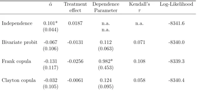
Table IV contains the key results. For each of the four copulas (independence, normal, Frank and Clayton), it lists the estimated α parameter, the implied average treatment effect of HMO on no ambulatory expenditure, the estimated dependence parameter, Kendall’s τ as well as the log-likelihood value. The ATE’s vary quite a bit, from +1.9 percent under independence to -2.6 percent in the Frank CBP model. Although the ATE estimates are consistently negative in CBP models with dependence, the size is cut by half when moving from the Frank CBP to the normal CBP model, and cut by half again when moving to the Clayton CBP.
Statistically, the Frank CBP has the largest log-likelihood value, although the differences are not large. A test of the Frank CBP against the independence CBP formally rejects the independence assumption. The chi-squared (1) - distributed likelihood ratio test statistic is 4.6, with p-value of 0.032. Similarly, the Frank dependence parameter is significantly greater than zero. The sign suggests positive self-selection: those who are more likely to opt for HMO have a higher than average probability of having no ambulatory expenses. If unaccounted for, the positive dependence between the unobservables in the two equations is captured by the effect estimate which is indeed found to be positive and even statistically significant in the independence model. Once endogeneity
is accounted for, the effect switches its sign but it is not statistically significant.
It is interesting to observe that the conclusion obtained from formal applications of hypothesis tests based on the normal CBP would be quite different, since the independence CBP cannot be rejected against the normal CBP model. Likelihood ratio andz-test statistics are both insignificant. As a consequence, one would be led to interpret the +1.9 percent ATE under independence as causal.
− − − − − − − − − Table V about here − − − − − − − − −
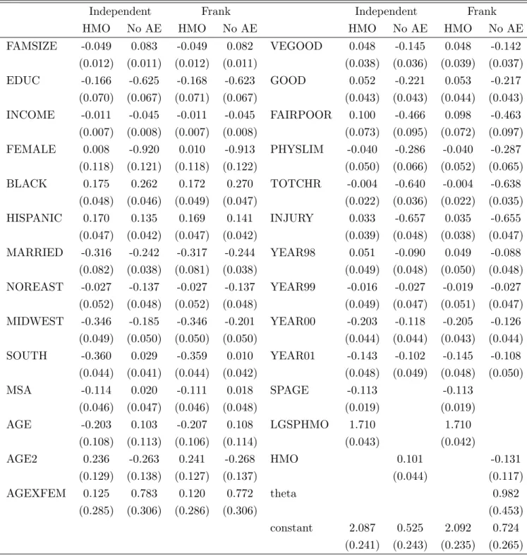
The full set of regression coefficients for the independence and Frank copula are displayed in Table V. Except for the HMO coefficient, there is not much difference between the size and precision of the estimated effects between the two models.
4
Discussion
The paper considers the problem of modeling and estimating the effect of a binary endogenous regressor on a binary outcome variable using copulas. The copula bivariate probit (CBP) model is an alternative to semi-parametric estimation of bivariate probit models (e.g. Murphy, 2007, Chen and Zhou 2007). It offers a relatively simple and parsimonious compromise between the standard bivariate probit model and these semi-parametric alternatives. The main benefits of CBP models are twofold. First, they make it relatively effortless to assess the sensitivity of results within a broader class of joint distributions for the stochastic errors. Second, by considering a number of
different copulas one can obtain, in a quasi-likelihood sense, a better approximation to the true underlying distribution.
The evidence provided in the paper, based on simulations and a real data application, suggests that CBP models work well in practice and provide a viable and simple alternative to the stan-dard bivariate probit approach. Of course, the bivariate probit can well be the best model in the considered class of CBP models. Even then, however, one does not know this before the analysis, and selecting from a larger menu of models is helpful for assessing the sensitivity of estimates to distributional assumptions.
The methods and models presented in the paper have at least two immediate extensions. First, they can be applied to cases where the outcome variable is an ordered response with more than two outcomes. For example, one can easily construct a model with ordered probit marginals for the outcome variable and binary probit marginal for the endogenous regressor. The ordered probit model has a latent variable representation as well. Let
y1∗ =xβ+αy2+ε1
The observed ordered responses y1 = 1,2, . . . , J are obtained from a threshold observation mecha-nism y1 = J X j=0 1(y1∗ > κj)
where κs,0 =−∞< κs,1 < . . . < κs,J =∞ partition the real line. It follows that
and
P(y1 =j, y2 = 1) =C(Φ(κj−xβ−α),1)−C(Φ(κj−1 −xβ−α),1)−P(y1 =j, y2 = 0)
Second, the copula approach can be easily extended to accommodate other marginal models, such as the logit or any other desired link function (Koenker and Yoon, 2009). A bivariate model with logit marginals is obtained by lettingF(ε1, ε2) = C[Λ(ε1),Λ(ε2)], where Λ(z) = exp(z)/(1 + exp(z)) is the cumulative density function of the logistic distribution. Alternatively, one could estimate the marginals semiparametrically, an approach that has been explored in other copula applications (e.g., Chen and Fan 2005).
A further potentially fruitful development explores copula mixture models, where the underlying joint distribution function of the unobservables is approximated by a finite mixture of parametric distribution functions that can differ both in their copula specification and in their parameters. Conceptually this is a very elegant approach as it dispenses with the need to select single copulas and moreover can in principle approximate the true joint distribution function to an arbitrary degree. The practical implementation may be very difficult, however, and related results from a study by Trivedi and Zimmer (2009) are not very encouraging.
5
References
Chen, S. and Y. Zhou (2007) Estimating a generalized correlation coefficient for a generalized bivariate probit model, Journal of Econometrics 141, 1100 - 1114.
multivariate copula models, Canadian Journal of Statistics 33, 389 - 414.
Chernoff, H. (1954) On the distribution of the likelihood ratio, Annals of Mathematical Statistics
25, 573-578.
Deb, P., M.K. Munkin and P.K. Trivedi (2006) Bayesian analysis of the two-part model with endogeneity: application to health care expenditure, Journal of Applied Econometrics, 21, 1081-1099.
Dormont, B., Geoffard, P.-Y. and K. Lamiraud (2009) The influence of supplementary health insurance on switching behaviour: evidence from Swiss data, Health Economics 18, 1339-1356.
French, M.T. and J.C. Maclean (2006) Underage alcohol use, delinquency, and criminal activity,
Health Economics 15, 1261-1281.
Gitto, L., D. Santoro and G. Sobbrio (2006) Choice of dialysis treatment and type of medical unit (private vs public), application of a recursive bivariate probit, Health Economics 15, 1251-1256.
Joe, H. (1997) Mutivariate Models and Multivariate Dependence Concepts, Chapman & Hall / CRC.
Jones, A.M. and O. O’Donnell (2002) Econometric Analysis of Health Data, Wiley
Koenker, R. and J. Yoon (2009) Parametric links for binary choice models: A Fisherian - Bayesian colloquy, Journal of Econometrics 152, 120-130.
Latif, E. (2009) The impact of diabetes on employment in Canada, Health Economics18, 577-589.
Lee, L.-F. (1983) Generalized econometric models with selectivity, Econometrica51, 507-512.
MacDonald, Z. and M.A. Shields (2004) Does problem drinking affect employment? Evidence from England, Health Economics13, 139-155.
Manning, W.G., Morris, C.N., Newhouse, J.P., et al. (1981) A two-part model of the demand for medical care: preliminary results from the Health Insurance Study. In: van der Gaag, J., Perlman, M. (eds.) Health, Economics, and Health Economics, North Holland, Amsterdam, 103-123.
Munkin, M.K. and Trivedi, P.K. (2008) Bayesian analysis of the ordered probit model with en-dogenous selection, Journal of Econometrics, 143, 334-348.
Murphy, A. (2007) Score tests of normality in bivariate probit models, Economics Letters 95, 374-379.
Nelson, R.B. (2006) An Introduction to Copulas, Springer, Berlin.
Prieger, J. (2002) A flexible parametric selection model for non-normal data with an application to health care usage, Journal of Applied Econometrics 17, 367-392.
Prokhorov, A. and P. Schmidt (2009) Likelihood based estimation in a panel setting: robustness, redundancy and validity of copulas, Journal of Econometrics 153, 93-104.
Sklar, A. (1959) Fonctions de r´epartition `a n dimensions et leurs marges,Publications de l’Institut
de Statistique de L’Universit´e de Paris, 8, 229-231.
Smith Conway, K. and A. Kutinova (2006) Maternal health: does prenatal care make a difference?,
Health Economics 15, 461-488.
Smith M.D. (2003) Modelling sample selection using Archimedean copulas, Econometrics Journal, 6, 99-123.
Smith M.D. (2005) Using copulas to model switching regimes with an application to child labour,
Economic Record, 81, S47-S57.
Trivedi, P.K. and Zimmer, D.M. (2007) Copula modeling: an introduction for practitioners,
Foun-dations and Trends in Econometrics, Volume 1, Issue 1.
Trivedi, P.K. and D. Zimmer (2009) Pitfalls in Modeling Dependence Structures: Explorations with Copulas. In: J. Castle and N. Shephard (eds.) The Methodology and Practice of Econometrics, Oxford University Press.
White, H. (1982) Maximum likelihood estimation of misspecified models, Econometrica50, 1-26.
Wilde, J. (2000) Identification of multiple equation probit models with endogenous dummy regres-sors, Economics Letters69, 309-312.
Zimmer, D.M. and Trivedi, P.K. (2006) Using trivariate copulas to model sample selection and treatment effects: application to family health care demand, Journal of Business and
Table I
Simulation Results for Normal CBP Data Generating process (ρ= 0.5, r=5000) ˆ β0 βˆ1 αˆ θˆ τ llik % pick n = 500 Normal 0.499 -0.504 0.512 0.497 0.335 -473.5 40.8 (0.107) (0.072) (0.226) (0.132) Frank 0.501 -0.507 0.527 3.419 0.333 -473.7 33.6 (0.108) (0.073) (0.233) (1.251) Clayton 0.467 -0.507 0.554 0.747 0.260 -474.1 25.5 (0.115) (0.074) (0.241) (0.370)
Independence 0.231 -0.527 1.120 n.a. n.a. -479.3 0 (0.086) (0.075) (0.145) n.a. n = 1000 Normal 0.500 -0.501 0.502 0.502 0.337 -950.7 48.6 (0.076) (0.050) (0.161) (0.093) Frank 0.503 -0.503 0.515 3.392 0.336 -951.0 31.6 (0.077) (0.051) (0.166) (0.859) Clayton 0.466 -0.504 0.546 0.721 0.259 -951.9 19.7 (0.082) (0.052) (0.171) (0.245)
Independence 0.228 -0.524 1.116 n.a n.a. -961.9 (0.059) (0.053) (0.101) n.a. n = 5000 Normal 0.500 -0.501 0.500 0.501 0.334 -4763.6 80.0 (0.034) (0.022) (0.071) (0.041) Frank 0.503 -0.504 0.514 3.313 0.333 -4765.2 16.4 (0.034) (0.022) (0.072) (0.367) Clayton 0.465 -0.504 0.546 0.691 0.256 -4769.8 3.6 (0.037) (0.023) (0.075) (0.103)
Independence 0.229 -0.523 1.110 n.a. n.a. -4817.3 (0.027) (0.023) (0.045) n.a.
Notes: The main entries in the table give the mean values of the statistics over repeated samples.
Standard deviations in parentheses. The true parameter values are β0 = 0.5, β1 = −0.5, and
Table II
Simulation Results for Frank CBP Data Generating Process (θ = 3.3,r=5000) ˆ β0 βˆ1 αˆ θˆ τ llik % pick n = 500 Normal 0.492 -0.498 0.503 0.490 0.330 -475.3 28.8 (0.107) (0.072) (0.221) (0.129) Frank 0.501 -0.501 0.503 3.465 0.337 -475.1 52.8 (0.106) (0.072) (0.224) (1.225) Clayton 0.457 -0.500 0.550 0.719 0.252 -476.1 18.4 (0.116) (0.074) (0.240) (0.370)
Independence 0.227 -0.521 1.101 n.a. n.a. -481.0 0 (0.084) (0.075) (0.143) n.a. n = 1000 Normal 0.489 -0.498 0.506 0.486 0.325 -954.3 28.0 (0.077) (0.051) (0.160) (0.093) Frank 0.499 -0.502 0.504 3.357 0.333 -954.0 61.4 (0.075) (0.051) (0.160) (0.826) Clayton 0.452 -0.500 0.557 0.672 0.246 -956.0 10.6 (0.084) (0.052) (0.175) (0.243)
Independence 0.226 -0.520 1.097 n.a n.a. -965.0 (0.060) (0.052) (0.101) n.a. n = 5000 Normal 0.490 -0.497 0.503 0.487 0.324 -4782.3 18.1 (0.034) (0.022) (0.069) (0.040) Frank 0.500 -0.501 0.501 3.309 0.333 -4780.6 81.3 (0.033) (0.023) (0.070) (0.351) Clayton 0.451 -0.499 0.557 0.647 0.243 -4791.0 0.6 (0.037) (0.023) (0.076) (0.100)
Independence 0.225 -0.518 1.095 n.a. n.a. -4833.7 (0.027) (0.023) (0.045) n.a.
Table III
Simulation Results for Clayton CBP Data Generating Process (θ= 1, r=5000) ˆ β0 βˆ1 αˆ θˆ τ llik % pick n = 500 Normal 0.513 -0.497 0.521 0.573 0.393 -465.1 19.4 (0.104) (0.072) (0.222) (0.124) Frank 0.507 -0.498 0.551 4.109 0.384 -465.6 9.2 (0.105) (0.073) (0.235) (1.427) Clayton 0.505 -0.501 0.501 1.088 0.341 -464.2 71.4 (0.108) (0.073) (0.222) (0.427)
Independence 0.203 -0.527 1.241 n.a. n.a. -473.0 0 (0.086) (0.076) (0.148) n.a. n = 1000 Normal 0.509 -0.497 0.524 0.570 0.388 -934.0 14.8 (0.073) (0.051) (0.160) (0.089) Frank 0.505 -0.498 0.554 3.964 0.380 -935.1 4.4 (0.073) (0.052) (0.169) (0.978) Clayton 0.501 -0.501 0.503 1.040 0.336 -932.3 80.8 (0.076) (0.052) (0.160) (0.290)
Independence 0.201 -0.526 1.238 n.a n.a. -949.1 (0.060) (0.053) (0.103) n.a. n = 5000 Normal 0.509 -0.496 0.522 0.570 0.386 -4681.0 2.0 (0.033) (0.022) (0.070) (0.038) Frank 0.505 -0.498 0.553 3.874 0.378 -4686.6 0.1 (0.033) (0.023) (0.074) (0.403) Clayton 0.500 -0.501 0.501 1.007 0.334 -4672.4 97.9 (0.034) (0.023) (0.070) (0.119)
Independence 0.200 -0.525 1.235 n.a. n.a. -4754.4 (0.027) (0.023) (0.046) n.a.
Table IV: Results for Absence of Ambulatory Expenditure Example ˆ
α Treatment Dependence Kendall’s Log-Likelihood
effect Parameter τ
Independence 0.101* 0.0187 n.a. n.a. -8341.6
(0.044) n.a. Bivariate probit -0.067 -0.0131 0.112 0.071 -8340.0 (0.106) (0.063) Frank copula -0.131 -0.0256 0.982* 0.108 -8339.3 (0.117) (0.453) Clayton copula -0.032 -0.0061 0.124 0.058 -8340.4 (0.105) (0.095)
* indicates statistical significance at the 5% level.
Table V: Full Regression Results for Absence of Ambulatory Expenditure
Independent Frank Independent Frank HMO No AE HMO No AE HMO No AE HMO No AE FAMSIZE -0.049 0.083 -0.049 0.082 VEGOOD 0.048 -0.145 0.048 -0.142 (0.012) (0.011) (0.012) (0.011) (0.038) (0.036) (0.039) (0.037) EDUC -0.166 -0.625 -0.168 -0.623 GOOD 0.052 -0.221 0.053 -0.217 (0.070) (0.067) (0.071) (0.067) (0.043) (0.043) (0.044) (0.043) INCOME -0.011 -0.045 -0.011 -0.045 FAIRPOOR 0.100 -0.466 0.098 -0.463 (0.007) (0.008) (0.007) (0.008) (0.073) (0.095) (0.072) (0.097) FEMALE 0.008 -0.920 0.010 -0.913 PHYSLIM -0.040 -0.286 -0.040 -0.287 (0.118) (0.121) (0.118) (0.122) (0.050) (0.066) (0.052) (0.065) BLACK 0.175 0.262 0.172 0.270 TOTCHR -0.004 -0.640 -0.004 -0.638 (0.048) (0.046) (0.049) (0.047) (0.022) (0.036) (0.022) (0.035) HISPANIC 0.170 0.135 0.169 0.141 INJURY 0.033 -0.657 0.035 -0.655 (0.047) (0.042) (0.047) (0.042) (0.039) (0.048) (0.038) (0.047) MARRIED -0.316 -0.242 -0.317 -0.244 YEAR98 0.051 -0.090 0.049 -0.088 (0.082) (0.038) (0.081) (0.038) (0.049) (0.048) (0.050) (0.048) NOREAST -0.027 -0.137 -0.027 -0.137 YEAR99 -0.016 -0.027 -0.019 -0.027 (0.052) (0.048) (0.052) (0.048) (0.049) (0.047) (0.051) (0.047) MIDWEST -0.346 -0.185 -0.346 -0.201 YEAR00 -0.203 -0.118 -0.205 -0.126 (0.049) (0.050) (0.050) (0.050) (0.044) (0.044) (0.043) (0.044) SOUTH -0.360 0.029 -0.359 0.010 YEAR01 -0.143 -0.102 -0.145 -0.108 (0.044) (0.041) (0.044) (0.042) (0.048) (0.049) (0.048) (0.050) MSA -0.114 0.020 -0.111 0.018 SPAGE -0.113 -0.113 (0.046) (0.047) (0.046) (0.048) (0.019) (0.019) AGE -0.203 0.103 -0.207 0.108 LGSPHMO 1.710 1.710 (0.108) (0.113) (0.106) (0.114) (0.043) (0.042) AGE2 0.236 -0.263 0.241 -0.268 HMO 0.101 -0.131 (0.129) (0.138) (0.127) (0.137) (0.044) (0.117) AGEXFEM 0.125 0.783 0.120 0.772 theta 0.982 (0.285) (0.306) (0.286) (0.306) (0.453) constant 2.087 0.525 2.092 0.724 (0.241) (0.243) (0.235) (0.265)
Standard errors in parentheses; the following variables are scaled by factor 10−1: EDUC, INCOME, AGEXFEM, AGE2.
−4 −2 0 2 4 −3 −2 −1 0 1 2 3 v1
Figure 1: 500 draws from a Frank Copula with Standard Normal Marginals, θ = 3.3. Linear regression line and locally weighted polynomial regression
−4 −2 0 2 4 −3 −2 −1 0 1 2 3 v1
Figure 2: 500 draws from a Clayton Copula with Standard Normal Marginals, θ = 1. Linear regression line and locally weighted polynomial regression