Accuracy of Bayes and Logistic Regression Subscale Probabilities for Educational and Certification Tests

(1)

Volume 21 Volume 21, 2016 Article 8 2016

Accuracy of Bayes and Logistic Regression Subscale Probabilities

for Educational and Certification Tests

Lawrence Rudner

Follow this and additional works at: https://scholarworks.umass.edu/pare Recommended Citation

Recommended Citation

Rudner, Lawrence (2016) "Accuracy of Bayes and Logistic Regression Subscale Probabilities for Educational and Certification Tests," Practical Assessment, Research, and Evaluation: Vol. 21 , Article 8. DOI: https://doi.org/10.7275/q7zz-d655

Available at: https://scholarworks.umass.edu/pare/vol21/iss1/8

This Article is brought to you for free and open access by ScholarWorks@UMass Amherst. It has been accepted for inclusion in Practical Assessment, Research, and Evaluation by an authorized editor of ScholarWorks@UMass Amherst. For more information, please contact [email protected].

(2)

A peer-reviewed electronic journal.

Copyright is retained by the first or sole author, who grants right of first publication to Practical Assessment, Research & Evaluation. Permission is granted to distribute this article for nonprofit, educational purposes if it is copied in its entirety and the journal is credited. PARE has the right to authorize third party reproduction of this article in print, electronic and database forms.

Volume 21, Number 8, July 2016 ISSN 1531-7714

Accuracy of Bayes and Logistic Regression Subscale

Probabilities for Educational and Certification Tests

Lawrence Rudner, The Arcturus Group

In the machine learning literature, it is commonly accepted as fact that as calibration sample sizes increase, Naïve Bayes classifiers initially outperform Logistic Regression classifiers in terms of classification accuracy. Applied to subtests from an on-line final examination and from a highly regarded certification examination, this study shows that the conclusion also applies to the probabilities estimated from short subtests of mental abilities and that small samples can yield excellent accuracy. The calculated Bayes probabilities can be used to provide meaningful examinee feedback regardless of whether the test was originally designed to be unidimensional.

Most tests are originally designed to provide only an overall score, but in recent years there has been a great deal of interest in also providing diagnostic feedback to the examinee. After studying for hours, spending a sum of money, and taking a long test, test takers understandably find it very unsatisfactory to receive just a single score, and especially if that score is simply categorized as failure. In that case, the test taker has no guidance for how to prepare for a retest.

Current approaches to identifying relative strengths and weaknesses of a test-taker are often not satisfactory to the measurement community. Estimates of subtest ability typically contain a great deal of measurement error and subtests are rarely equivalent across forms. More importantly, improvement in a weak area may not be as useful for total score gains as improvement in a strength.

An alternative form of feedback could change the focus from an examinee’s relative strengths and weaknesses to an examination of the probabilities of passing the entire test given their responses to items on subscales. For example: “Someone with your responses to algebra questions has a 40% chance of passing the test while someone with your responses to arithmetic

questions has a 90% chance of passing.” Phrased another way, “If nothing changes, then based on your responses to algebra questions you have a 40% chance of passing and based on your responses to arithmetic questions, you have a 90% chance of passing.” This changes the focus of the feedback to better match the goal of the examinee – to pass or do well on the examination. This assumes, of course, that good probability estimates can be obtained.

Two approaches to computing such subscale probabilities are naïve Bayes classifiers and Binary Logistic Regression. Both of these latent classification techniques are used in machine learning where there is a series of dichotomous observations (e.g. the presence or absence of words or right/wrong scoring of test questions) and a dichotomous classification (e.g. hire/don’t hire or pass/fail).

While there is a rich literature on these methods as applied to machine learning, it is not known whether the learnings from this literature apply to educational assessment. This paper presents these two models, highlights what is known from machine learning, demonstrates these procedures with two very different cognitive tests, and examines whether expectations

(3)

from the machine learning literature also apply to cognitive assessment.

Related literature

Machine learning has been broadly defined as “computational methods using experience to improve performance or to make accurate predictions” (Mohri, Rostamizadeh & Talwalkar, 2012). Perhaps the best known application in the assessment field is the use of computers to score written essays. An initial set of previously scored essays in response to a given prompt are used to train a model for that prompt. Often a second set is used to validate the model and then one or more human raters are replaced by the model (Shermis & Burstein, 2003). In this context, the words and phrases of the essays are observations and the presence or absence of certain words and phrases can be used to grade the materials. Similarly, responses to test questions are observations and the presence or absence of a correct response can be used to help classify the test taker as being a member of one group (e.g. pass) or another (e.g. fail). In this paper, we will be concerned with right/wrong scoring and the probability of passing the overall test. This is a latent class model (Lazarsfeld and Henry, 1968) where the underlying trait (pass/fail) is dichotomous and the observations (right/wrong scored test questions) are also dichotomous.

Two popular models from the machine learning literature are Bayes classifiers and Binary Logistic Regression. Vomlel (2004) and Rudner (2009) present Bayes classifiers as a measurement model. Zwinderman (1991) and others discuss logistic regression as a measurement model and its relationship to the Rasch Model.

The task is to calculate the probability of passing the entire test based on the responses to the individual items on a subtest. Under the Bayesian approach, we calculate the probability of being in group mk given the response vector, z, as.

| _∑ |

|

where P(z|mk) is the probability of the response vector for masters and for non-masters and P(mk) is the prior probability of group membership. P(z|mk) and P(mk) are learned from training data which could be gathered as part of a pretest or based on past data. In practice,

P(z|mk) cannot be directly estimated. Values are needed for every possible response vector. For a test of length n, there are 2n possible vectors. Thus, for a 15 item subtest, that would be 215 = 32,768 possible response vectors. Each possible vector needs a large number of respondents in each group in order to obtain stable conditional probability estimates. While such data gathering is impractical for a short cognitive test, it is impossible in text classification where a corpus might contain several thousand different words.

One solution is to evoke the Naïve Bayes Assumption:

| |

where the subscript i denotes individual test questions and P(zi | mk) is the p-value conditioned on group

members, i.e. the p-values for masters and the p-values for non-masters. This assumption, which is shared with item response theory and confirmatory factor analysis, is also known as the local independence assumption, i.e. the items are independent of each. While this assumption might be an issue when analyzing questions based on the same reading passage, it is not usually a problem in assessment.

The Naïve Bayes approach does not rely on the usual assumptions of item response theory (IRT). Unidimensionality and monotonically increasing probabilities are not assumed. Questions measuring different skills can be combined and items that are harder for more capable individuals can be used. Most importantly, relative to IRT, sample sizes to train the model can be very small. Typically, a representative sample of only 30 to 50 masters and a similar number of non-masters are needed to compute stable conditional p-values. Because of the small number of non-masters, the American Board of Anesthesiologists cleverly uses a proxy for non-masters by subtracting a constant from the well-estimated probabilities for masters (Harman, 2014).

In the machine learning literature, with its large number of “items”, the Naïve Bayes assumption is almost always violated. With text, for example, words often appear multiple times and often some words almost always appear with other words. The result is a pushing of the probabilities away from .5 and toward the tails, 0.0 and 1.0. Suppose, for example, we have a classifier whose normalized probability for masters = .8.

(4)

Practical Assessment, Research & Evaluation, Vol 21, No 8 Page 3 Rudner, Accuracy of Bayes and Logistic Regression Subscale Scores

When that item is repeated it counts twice in the calculation and its effective probability for masters becomes

. 8

. 8 . 2 .94

The classifications (e.g. pass or fail) are not affected (Domingos & Pazzani, 1997). An examine whose true probability is .55 and whose calculated probability is .80 will still receive the same mastery classification. However, often the probabilities can’t be trusted and a variety of approaches have been offered to improve the calculated probability estimates (Schneider, 2005; Zadronzny and Elkan, 2002).

A natural question is whether the concern also holds true for cognitive tests. That question is answered in this paper using an approach outlined by Zadrozny and Elkan (2001, 2002). Actual probabilities are computed by placing groups of examinees into relatively homogeneous bins based on their calculated probabilities. Within each bin, the actual probability is the percent of people possessing the desired trait, e.g. passing the test. That value can be compared to the mean calculated probability within the bin to assess accuracy as a function of calculated probabilities. Regressing actual onto calculated probabilities yields a function that can be used to provide adjusted (corrected) probabilities. The use of bins to estimate actual probabilities was applied as part of this paper.

A popular alternative to the Bayes classifier approach from the machine learning literature is the use of Binary Logistic Regression (Hosmer & Lemeshow). Under this model, the probability of being a master, given the response vector z is

|

1

where g(z) = β0 + β1z1 + β2z2 + … + βjzj. The

probability of being a non-master, then is

| 1 | .

Logistic regression does not rely on the usual assumptions of models based on ordinary least squares. Linearity, normality, homoscedasticity, and measurement level are not assumed. It does, however, require the absence of multicollinearity and relatively large datasets, two to six times the data required for

simple regression based on ordinary least squares. Multicollinearity will not be a problem for most properly assembled cognitive assessments. Rarely can the performance on one item be accurately predicted from the results of two or more other items. The sample size issue is addressed in this paper.

The practical issue with logistic regression is model specification. An underspecified model will produce biased estimates and an over specified model will have less precise estimates. This will be a function of the size of the subtest, the size of the sample, and the relationship of the items within the subtest.

Binary logistic regression and Bayes classifiers are often compared. Logistic regression is often called a discriminative classifier and Bayes a generative classifier. Logistic regression directly estimates P(mk | z) whereas Naïve Bayes generates P(mk | z) from P(z| mk) and P(mk). In their seminal study comparing Logistic Regression and Naive Bayes classifiers, Ng & Jordon (2002) draw several important conclusions based on mathematical derivations. Through an analysis of 15 different datasets, they then provide empirical support for those conclusions. Specifically, they show

1. With large numbers of training samples, logistic regression classifiers have less classification error than Naïve Bayes classifiers, although that difference is not very large

2. As training sample size increases, Naïve Bayes classifiers converge to their highest accuracy level faster than logistic classifiers.

Thus, Bayes initially does better, but as the number of training examples increases, Logistic Regression classifiers eventually catch up and overtake Bayes classifiers in terms of the percent of cases properly classified. Other studies directly comparing Bayes and Logistic Regression classifiers with multiple datasets and finding the same results include Halloran (2009) and Sam, Karthi and Anu (2015).

Research questions

While much about logistic regression and Bayes classifiers is known and accepted as fact in machine learning applications, we do not know if these same facts hold true for use with cognitive tests. Relative to most datasets in machine learning, cognitive tests, and especially content based subtests, have few items and

(5)

probably less of a local independence problem. Thus, this paper asks:

1. For large calibration samples, do logistic regression and Bayes classifiers provide accurate classifications and accurate probability estimates for educational tests and subtests?

2. How does the classification accuracy and

probability estimate accuracy vary as a function of sample size for education tests and subtests?

Method

Data from two different standardized examinations were used, one is the final and only examination for an on-line course (Test A), the other is a well-known and highly-respected certification examination (Test B). For each test, the data included each respondent’s right/wrong responses and whether or not the individual passed the examination. With the large number of examinees taking these tests, there will be more than enough data to compute stable accuracy estimates.

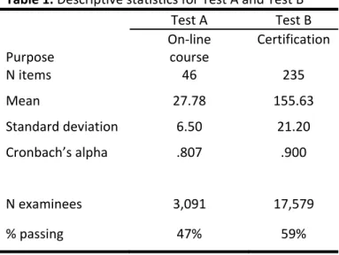
Descriptive statistics are shown in Table 1. The on-line course examination, Test A, is composed of 46 questions, has a marginally adequate reliability, and a pass rate of about 50%. The certification test, Test B, is composed of 235 operational questions, has good reliability, and a low pass rate of approximately 60%.

Table 1. Descriptive statistics for Test A and Test B Purpose Test A Test B On‐line course Certification N items 46 235 Mean 27.78 155.63 Standard deviation 6.50 21.20 Cronbach’s alpha .807 .900 N examinees 3,091 17,579 % passing 47% 59%

Statistics concerning the subtests are shown in Table 2. The Cronbach alpha reliabilities and difficulties of the subtests are not consistent, and as expected with the smaller number of items, some of the reliabilities are low. The subtests vary from 5 to 21 items. The percent

of bivariate item correlations after controlling for total score that are greater than .2, shown in the last column, is one measure of the severity of violating the local independence assumption. Thus, subskills 2 and 3 for Test A appear to have both a few number of items and probable notable violations of local independence. While Test B has eight subtests, for simplicity only the five subtests the fewest number of items were chosen for this analysis. The subtests reliabilities for Test B are extremely low, especially given their lengths.

Table 2. Subscore statistics Test Subskill N items Reliability Mean % correct % rxy.z>.2 A 1 16 .536 72% 0% 2 5 .341 60% 70% 3 6 .227 46% 53% 4 19 .730 55% 0% B 1 19 .163 72% 0% 2 21 .279 64% 0% 3 21 .164 74% 0% 4 21 .361 64% 0% 5 12 .269 63% 0%

Binary logistic regression and Naïve Bayes classifiers were applied to the subtest data. SPSS was used to apply the Binary Logistic Regression (BLR) and the freeware MDT Tools (Rudner, 2010) were used to apply Naïve Bayes (NB). Because the literature suggests sensitivity to sample size, random samples of 50, 100, 200, 500, and 1000 examinees were drawn for calibrating the BLR and NB models. Conditional probabilities were computed based on the masters and non-masters within each calibration sample. Thus, for test A with its 47% pass rate, the calibration sample of approximately 24 of the 50 examinees were used to compute the conditional p-values for masters for the first run. For each run, the remaining examinees not in the calibration sample were used as validation samples. Thus, the calibration and validation samples were independent, although, for the purpose of evaluating accuracy, this is not a requirement as long as the regression model is properly specified (Zadrozny & Elkan, 2002).

In order to compute actual probabilities and then compare actual to calculated, examinees were placed into one of twenty-one bins based on their calculated probabilities. The first and last bins were p=.025 in width (i.e. p< .025 and p> .975) and the rest were p=.05

(6)

in width (e.g. .025 to .0749 and .075 to .1249). The first and last bins were smaller because classifiers are able to identify clear masters and clear non-masters. It is not unusual for 10 to 20 percent of the examinees to be classified into each of the bins at the tails.

Other approaches to forming bins, including the Pool Adjacent Violators (PAV) algorithm (Ayer, Brunk, Ewing, Reid, & Silverman, 1955) and forming overlapping bins of 100 respondents after sorting in a manner analogous to moving averages, were tried and rejected. All approaches yielded similar results, so the simplest approach was used. What was critical was the bins were homogenous in terms of their probabilities, the probabilities were monotonically increasing, and that the samples sizes were adequate to form stable estimates.

Results

Ideally, the calculated probabilities should equal the actual probabilities. That is, the mean estimated probability for each bin should equal the actual percent of examinees in the bin that passed. The figures below present the relationships between calculated and predicted probabilities. On all the figures the 45-degree dotted line represents x=y, the line of perfect calculated probabilities.

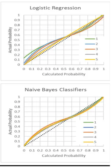
Figures 1 and 2 show the relationship between actual and calculated probabilities for each subtest using BLR and NB classifiers and a relatively large calibration sample size of 500 examinees. All subtests have great accuracy. The worst, as indicated by deviations from the 45-degree line, are Subtest 2 of Test A which has 5 items, using BLR, and subtest 3 of Test B which has 21 items, using NB. Note that subtests 2 and 3 of Test A, which have the highest potential of violating local independence where extremely accurate using NB.

The accuracy for these two runs are summarized in Tables 3 and 4. The Accuracy column refers to the percent of examinees that are correctly classified and is computed as the number of test takers with a probability greater than .5 that passed plus the number of test takers with a probability less than .5 that failed divided by the total number of examinees. Subtests are not expected to accurately predict who passes the overall test. For any test, there are usually test takers that

do well on one subtest and poorly on the others and it is for that reason diagnostic feedback is needed. Further, if a subtest predicted overall success with high accuracy, there would be no need for the other subtests.

Figure 1. Calibration accuracy by calculated probabilities for subtests of Test A and calibration sample sizes of 500 examinees

The statistic of interest is the root mean square error (RMSE) which is a measure of the quality of the probabilities whereas Accuracy is a measure of the quality of the classification. RMSE compares the actual and mean calculated probabilities averaged over the twenty-one bins and weighted by the number of examinees in each bin.

(7)

Figure 2. Calibration accuracy by calculated probabilities for subtests of Test B and calibration sample sizes of 500 examinees

For a sample size of 500, BLR and NB have about the same classification accuracy. For every subtest of Test A and for 3 of the 5 subtests of Test B, BLR does a better job of estimating probabilities, although all of the error values for both methods are very small.

Table 3. Accuracy for Test A, calibration size 500

Subtest Logistic Regression Naive Bayes

Accuracy RMSE Accuracy RMSE

1 80% .053 80% .070

2 72% .050 72% .058

3 68% .053 68% .062

4 86% .034 87% .064

Table 4. Accuracy for Test B, calibration size 500

1 64% .073 64% .044

2 68% .081 69% .059

3 64% .056 66% .069

4 71% .038 72% .048

5 68% .034 69% .063

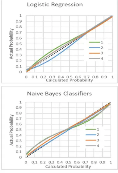
Calibrating with 100 examinees, however, results in a different finding. As shown in Figures 3 and 4, BLR does not work as well as NB for Test A when the calibration sample size is 100. With BLR, subtests 3 and 4 of Test A are fine, but the calculated probabilities are not accurate for subtests 1 and 2. As shown in Table 5, the classification accuracies are about the same, but NB has less error in the calculated probabilities on all four subtests.

Figure 3. Calibration accuracy by calculated probabilities for subtests of Test A and calibration sample sizes of 100 examinees

(8)

Table 5. Accuracy for Test A calibration size 100 Subtest Logistic Regression Naive Bayes

1 75% .151 79% .076

2 72% .170 72% .070

3 68% .084 67% .070

4 82% .116 85% .066

Similar results are found for Test B when calibrating on 100 examinees. While both BLR and NB yield inflated calculated probabilities for values below .5 and deflated probabilities above .5, NB outperforms BLR for every subtest.

Figure 4. Calibration accuracy by calculated probabilities for subtests of Test B and calibration sample sizes of 100 examinees

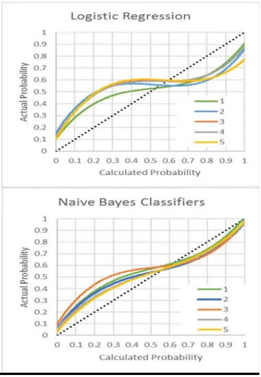
Figure 5 and Table 7 present the accuracy as a function of sample size for BLR and NB applied to subtest 1 of Test A. There is no accuracy plot for a

calibration size of 50 for BLR because all the examinees had calculated probabilities less than .025 or greater than .975.

Table 6. Accuracy for Test B calibration size 100

1 63% .144 61% .095

2 62% .234 65% .101

3 58% _.185 _63% _.147

4 64% .203 71% .090

5 57% _.202 _69% _.077

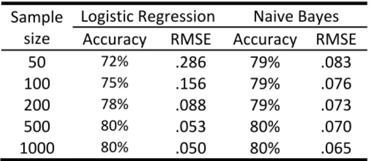
The data supports Ng and Jordan’s (2002) finding that, as the size of the training group increases, NB initially classifies more accurately but BLR catches up and performs better with larger samples (see Table 7).

Figure 5. Accuracy as a function of calibration sample size, Test A, Subtest 1

(9)

A similar trend is found for the accuracy of the probabilities. The regression lines in Figure 5 all become closer to the 45-degree line, i.e. more accurate, as the calibration sample sizes increase.

Table 7. Accuracy as a function of sample size for Test A, Subtest 1

Sample size

Logistic Regression Naive Bayes

50 72% .286 79% .083

100 75% .156 79% .076

200 78% .088 79% .073

500 80% .053 80% .070

1000 80% .050 80% .065

Similar results were found for Subtest 1 of Test B. The regression lines in Figure 6 all become closer to the 45-degree line, i.e. more accurate, as the calibration

Figure 6. Accuracy as a function of calibration sample size, Test B, Subtest 1

sample sizes increase. The regression lines for NB and the associated RMSE values show better accuracy for the NB probabilities until the sample size, for this test, is 1000. BLR with a sample size of 1000 outperforms all other models.

Table 8. Accuracy as a function of sample size for Test B, Subtest 1 Sample size Logistic Regression Naive Bayes

50 62% _.370 _59% _.159 100 63% _.144 _61% _.095 200 62% _.102 _62% _.064 500 64% _.073 _64% _.044 1000 64% _.032 _65% _.040

Discussion

Binary Logistic Regression and Naïve Bayes classifiers were applied to subtests from an on-line final course examination and from a highly-respected certification examination. Consistent with the findings in the machine learning literature, Naïve Bayes classifiers initially outperform logistic regression classifiers in terms of classification accuracy, as well as the accuracy of the probabilities, as calibration sample size increases. With large calibration sample sizes Logistic Regression outperforms Naïve Bayes.

In addition to calibration sample size, accuracy is also a function of subtest length. Accuracy does not appear to be related to subtest reliability, difficulty, or local dependency. Accuracy does vary by test length, although not as dramatically as one might expect. With adequate calibration sample sizes, the calculated probabilities were all very accurate.

One concern that motivated this study was whether the probabilities were sufficiently accurate for use as feedback to test takers. It is known from the machine learning literature when analyzing large bodies of text that Bayes classifiers tend to push probabilities toward the tails when there are violations of the local independence assumption, which is almost always the case. With relatively short subtests in this study, there was no pushing toward the tails, even with subtests having local dependencies.

Based on the literature and this study, it is clear that Naïve Bayes is the model of choice when the sample

(10)

sizes are relatively small. The calculated probabilities and the classification accuracies are good. An important finding is that Naïve Bayes probabilities were accurate for all subtests when the calibration sample size was 100, i.e. approximately 50 per group. Except for one subtest, excellent results were also obtained with a calibration sample size of 50. With larger calibration samples, logistic regression out performs Naïve Bayes, but the difference is not overwhelming. With large calibration samples, either model could be used.

If one is concerned about providing very accurate probabilities, then one could transform the calculated probabilities based on the regression of actual percent of masters on the mean calculated probabilities. However, this would probably require 300 or more examinees to properly form bins and at 300 examinees the calculated probabilities will often be sufficiently accurate. A ten percent error in the reported probabilities would not make a difference for most test takers.

A major advantage of the Naïve Bayes approach is the fact that accurate estimates can be obtained with very small calibration sample sizes. This is not surprising because the Bayes approach is only trying to trying to obtain accurate estimates for a limited number of data points. In this study only two groups, masters and non-masters, were estimated. The small calibration sample size makes the approach feasible for smaller testing programs and in all cases, it makes pilot data collection relatively easy.

Another advantage of the Naïve Bayes approach that there is no unidimensionality assumption. Items from different content areas can be combined and once calibrated can yield accurate classification probabilities. One possibility is to use a small sample of items as a placement test or as a routing test in an intelligent tutoring system.

One possible limitation of the Naïve Bayes approach is the lack of the parameter invariance property which makes it is relatively easy to always place item parameters on the same scale. However, conditional p-values obtained from non-equivalent groups can be placed on the same scale (see Guo, Talento-Miller, and Rudner, 2009). This allows items to be combined to yield a subtest with known characteristics and allow probabilities to be computed based on a single reference group. Another approach might be to convert IRT parameters to conditional

p-values based on the cut score and a fixed ability distribution.

References

Ayer, M., Brunk, H.D., Ewing, G.M., Reid, W.T., Silverman, E. (1955). An empirical Distribution function for Sampling with Incomplete Information.

The Annals of Mathematical Statistics” 6(4), 641-647. Domingos, P., & Pazzani, M. (1997). On the Optimality of

the Simple Bayesian Classifier under Zero-One Loss.

Machine Learning, 29, 103-13. Available online:

http://www.ics.uci.edu/~pazzani/Publications/mlj97-pedro.pdf

Guo, F, Talento-Miller, E., and Rudner, L (2009). Scaling Item Difficulty Estimates from Nonequivalent

Groups. GMAC Research Report RR-09-03. Available online:

http://www.gmac.com/~/media/Files/gmac/Researc h/research-report-series/rr0903_scalingitems_web.pdf Halloran, J. (2009). Classification: Naive Bayes vs logistic

regression. Univ. Hawaii, Available online:

http://melodi.ee.washington.edu/~halloj3/pdfs/john THalloranFinalPaperUhEE645Fall2009.pdf

Harman, A. (2014). Personal communication.

Hosmer, D. W., & Lemeshow, S. (2000). Applied logistic regression. New York: Wiley.

Hu, D (2011). How Khan Academy is using Machine Learning to Assess Student Mastery. Available online:

http://david-hu.com .

Lazarsfeld, P.F., and Henry, N.W. (1968). Latent Structure Analysis. Boston: Houghton Mill.

Mohri M., Rostamizadeh, A. and A. Talwalkar. Foundations of Machine Learning. MIT Press, 2012.

Ng, A.Y. & M.I. Jordan (2002). On discriminative vs. generative classifiers: A comparison of logistic regression and naive Bayes. Advances in neural information processing systems, 14, 841. Available online:

http://www.robotics.stanford.edu/~ang/papers/nips 01-discriminativegenerative.pdf

Rudner, L.M. (2009). Scoring and classifying examinees using measurement decision theory. Practical Assessment, Research & Evaluation, 14(8). Available online:

http://pareonline.net/getvn.asp?v=14&n=8 Rudner, L.M. (2010) Tools for applying Measurement

Decision Theory. Available online:

(11)

Sam, G., Karthi, M. and Anu, M. (2015). A statistical comparison of logistic regression and different Bayes classification methods for machine learning. ARPN Journal of Engineering and Applied Science, 10(14). Available online: https://www.researchgate.net Schneider, K. M. (2005). Techniques for improving the

performance of naive Bayes for text classification. In

Computational Linguistics and Intelligent Text Processing (pp. 682-693). Springer Berlin Heidelberg. Available online:

http://citeseerx.ist.psu.edu/viewdoc/download?doi=1 .1.1.59.2085&rep=rep1&type=pdf

Shermis, M.D. & J. Burstein (Eds.) (2003). Automated essay scoring: A cross-disciplinary perspective. Mahwah, NJ: Lawrence Erlbaum Associates.

Vomlel, J. (2004). Bayesian networks in educational testing. International Journal of Uncertainty, Fuzziness and Knowledge-Based Systems,12(supp01), 83-10 . Available online:

Zadrozny, B., & Elkan, C. (2001). Obtaining calibrated probability estimates from decision trees and naive Bayesian classifiers. International Conference on Machine Learning (pp. 609–616). Available online:

Zadrozny, B., & Elkan, C. (2002). Transforming classifier scores into accurate multiclass probability estimates. In

Proceedings of the Eighth ACM SIGKDD international conference on Knowledge discovery and data mining (pp. 694-699). ACM. Available online:

Zwinderman, A. H. (1991). A generalized Rasch model for manifest predictors. Psychometrika, 56(4), 589-60

Acknowledgements

The author wishes to thank Brian Kuhlman and Carl Setzer for their suggest improvements to an earlier draft of this paper and Pamela Getson for her insightful critique and improvements of this document.

This research was funded by Western Governors University which is not in any way responsible for any of the opinions or findings in this paper.

Citation:

Rudner, Lawrence. (2016). Accuracy of Bayes and Logistic Regression Subscale Probabilities for Educational and Certification Tests. Practical Assessment, Research & Evaluation, 21(8). Available online:

http://pareonline.net/getvn.asp?v=21&n=8 Author

Lawrence Rudner The Arcturus Group LMRudner [at] gmail.com