HAL Id: hal-02100819
https://hal.archives-ouvertes.fr/hal-02100819v2
Submitted on 29 Jan 2020HAL is a multi-disciplinary open access archive for the deposit and dissemination of sci-entific research documents, whether they are pub-lished or not. The documents may come from teaching and research institutions in France or abroad, or from public or private research centers.
L’archive ouverte pluridisciplinaire HAL, est destinée au dépôt et à la diffusion de documents scientifiques de niveau recherche, publiés ou non, émanant des établissements d’enseignement et de recherche français ou étrangers, des laboratoires publics ou privés.
Gaussian process optimization with failures:
classification and convergence proof
François Bachoc, Céline Helbert, Victor Picheny
To cite this version:
François Bachoc, Céline Helbert, Victor Picheny. Gaussian process optimization with failures: clas-sification and convergence proof. Journal of Global Optimization, Springer Verlag, In press. �hal-02100819v2�
Gaussian process optimization with failures: classification and
convergence proof
F. Bachoc1, C. Helbert2, V. Picheny3
1 Institut de Math´ematiques de Toulouse, Universit´e Paul Sabatier 2 Univ. de Lyon, Ecole Centrale de Lyon, CNRS UMR 5208,
Institut Camille Jordan, 36 av. G. de Collongue F-69134 Ecully cedex, FRANCE 3 PROWLER.io, Cambridge, UK
January 29, 2020
Abstract
We consider the optimization of a computer model where each simulation either fails or returns a valid output performance. We first propose a new joint Gaussian process model for classification of the inputs (computation failure or success) and for regression of the performance function. We provide results that allow for a computationally efficient maximum likelihood estimation of the covariance parameters, with a stochastic approx-imation of the likelihood gradient. We then extend the classical improvement criterion to our setting of joint classification and regression. We provide an efficient computation procedure for the extended criterion and its gradient. We prove the almost sure conver-gence of the global optimization algorithm following from this extended criterion. We also study the practical performances of this algorithm, both on simulated data and on a real computer model in the context of automotive fan design.
1
Introduction
Bayesian optimization (BO) is now established as an efficient tool for solving optimization problems with non-linear objectives that are expensive to evaluate. A wide range of applica-tions have been tackled, from hyperparameter tuning of machine learning algorithms [31] to wing shape design [16]. In the simplest BO setting, the aim is to find the maximum of a fixed unknown function f :D → R, where D is a box of dimension d. Under that configuration, the classical Efficient Global Optimization [EGO, 13] and its underlying acquisition function Expected Improvement (EI) are still considered state-of-the-art.
Several authors have adapted BO to the constrained optimization framework, i.e. when the acceptable design space A ⊂ D is defined by a set of non-linear, expensive-to-compute equations c:
A={x∈ D s.t. c(x)≤0},
either by adapting the EI function [30, 29, 6, 11, 25] or by proposing alternative acquisition functions [24, 12].
We consider here the problem of crash constraints, where the objective f is typically evaluated using a computer code that fails to provide simulation resultsf(x) for some input
conditionsx. We write A of the form
A={x∈ D;s(x) = 1}
wheres:D → {0,1} is a fixed unknown function.
We assume that, for eachx∈ D, a single computation provides the pair (s(x),1s(x)=1f(x)). Hence, it is as costly to see if a simulation at x fails as to observe the simulation result
f(x) when there is no failure. A typical example of failure might be a computational fluid dynamics (CFD) solver that does not converge. This convergence failure could be caused by an overly large time-step yielding an instability in the numerical scheme and a divergence, or by an inadequate mesh close to the boundary of the domain (see also the discussions in [28]). Another typical example of failure is when f(x) provides the numerical performance (e.g. the empirical risk) of a complex machine learning model (e.g. a deep neural network) depending on architecture parameters in x [15]. The computation of f(x) then relies on a gradient or stochastic gradient descent, using retro-propagation in the case of deep learning, for example. In this case, a failure occurs when the gradient descent does not converge, so that there is no observable value off(x) at convergence. In these two examples, we note that it is no less costly to observe a failure of the forms(x1) = 0 than to successfully observef(x2) withs(x2) = 1.
This optimization problem with failures was considered first by [10], where a Gaussian process classifier [GPC, 22] was used together with a spatialized EI. [17] also proposed the use of a GPC with EI, modified using an asymmetric entropy to limit as much as possible the computational resources spent on crashed simulations. However, both approaches rely on expensive Monte Carlo simulations, which make them impractical in some cases, and do not provide any convergence guarantee.
The contribution of this paper is two-fold. First, a new GPC model is proposed, where a latent GP is simply conditioned on the signs of the observations instead of their values. Its likelihood function maximization is studied, as well as its use to predict the feasibility proba-bility (i.e. crash likeliness) of a new designx. Second, leveraging recent results on sequential strategies [2], we propose an algorithm in the form of EGO with guaranteed convergence.
The outline of this paper is as follows. First, we introduce our GPC model (Section 2) and its use in a Bayesian optimization algorithm (Section 3). Section 4 states our main consistency result. Finally, our algorithm is illustrated on several simulated toy problems (Section 5), and applied to an industrial case study (Section 6). A conclusion is given in Section 7. All the proofs are deferred to the appendix.
2
A Classification model for crash constraints
This section presents our classification model used to characterize the feasible space A. It takes the classical form of a GPC with a latent GP, but conditioned solely on pointwise observations of its sign.
2.1 Conditioning GPs on observation signs
LetZ be a Gaussian process onD that has a constant mean function with valueµZ ∈Rand stationary covariance function kZ. Given a set of points x
observations Zn = (Z(x1), . . . , Z(xn))>, GP regression typically amounts to using the
pos-terior mean mZn(x, zn) = E(Z(x)|Zn = zn) and variance kZn(x) = Var(Z(x)|Zn = zn), for
zn∈Rn.
Now, in the classification setting,Z is a latent process andZnis not available. We propose
here to predict 1Z(x)>0 given the sign of Zn; that is, we consider the conditional non-failure
probability
Pnf(x) =P(Z(x)>0|sign(Zn) =sn),
where sn = (i1, . . . , in)> with i1, . . . , in ∈ {0,1} and sign(v) = (1v1>0, . . . ,1vn>0)
> for v =
(v1, . . . , vn)∈Rn.
To our knowledge, there is no exact integral-free expression of Pnf(x). The following lemma provides an expression of Pnf(x) that is more amenable to numerical approximation. Lemma 1. For sn∈ {0,1}n, letφZsnn be the conditional p.d.f. ofZngiven sign(Zn) =sn. Let
us define, for a∈R, b≥0, ¯ Φa b = ( 1−Φ ab if b6= 0 1−a>0 if b= 0 ,
where Φis the standard Gaussian c.d.f. Then we have
Pnf(x) = Z Rn φZn sn(zn) ¯Φ −mZn(x, zn) p kZ n(x) ! dzn.
Proof. The proof is deferred to Appendix A.
Because of Lemma 1, we suggest the following algorithm to approximate Pnf(x). Algorithm 1.
1. Samplezn(1), . . . , z(nN)∈Rn from the p.d.f. φZsnn.
2. For anyx∈ D, approximatePnf(x) by
d Pnf(x) = 1 N N X i=1 ¯ Φ −m Z n(x, z (i) n ) p kZ n(x) ! .
The benefit of Algorithm 1 is that Step 1, which is the most costly, has to be performed only once (independently of x ∈ D). In this step, zn(1), . . . , zn(N) can be sampled either by a
basic rejection method (samplingZnfrom its Gaussian p.d.f. φZn until the signs ofZnmatch
i1, . . . , in), or by a more advanced rejection method called Rejection Sampling from the Mode
(RSM) [19], or by more involved Markov Chain Monte Carlo (MCMC) methods [4, 33, 23]; see also their presentations in [18]. Step 2 is not costly and can be repeated for many inputs
2.2 Likelihood computation and optimization
Let {kZθ;θ ∈ Θ} be a set of stationary covariance functions on D with Θ ⊂ Rp. Typically,
θ consists of an amplitude term and one or several lengthscale terms [26, 27]. We aim at selecting a constant mean function forZ with valueµ∈Rand a covariance parameterθ. Let us first consider two pairs (θ1, µ1),(θ2, µ2) ∈ Θ×R for which kθ1Z/kθ1Z(0) = kθ2Z/kθ2Z(0) and
µ1/(kZθ1(0))1/2 =µ2/(kθ2Z(0))1/2. Then, we can check that the distribution of the sign process {1Z(x)>0;x∈ D}is the same whenZ has mean and covariance functionµ1 andkθ1 orµ2 and
kθ2. Hence, it is sufficient to let {kθZ;θ ∈Θ} be a set of stationary correlation function and
to letµ∈Rbe unrestricted.
Forsn∈ {0,1}n, letPµ,θ(sign(Zn) =sn) be the probability that sign(Zn) =sn, calculated
when Z has mean function µ and covariance function kθ. Then, the maximum likelihood
estimators forµand θ are
(ˆµ,θˆ)∈ argmax (µ,θ)∈R×Θ
Pµ,θ(sign(Zn) =sn). (1)
The likelihood criterion to optimize is the probability of an orthant ofRn, evaluated under
a multidimensional Gaussian distribution. Several advanced Monte Carlo methods exist to approximate this probability [4, 7, 1]. In addition, stochastic approximations of the gradient ofPµ,θ(sign(Zn) =sn) with respect to (µ, θ) can be obtained from conditional realizations of
Zn given sign(Zn) =sn. Calculations are provided in Appendix B.
2.3 Comparison with classical GPC
The model in Sections 2.1 and 2.2 can be written as
Ii =1Z(xi)>0 fori= 1, . . . , nand I =1Z(x)>0, (2)
whereI1, . . . , In∈ {0,1} are observed andI ∈ {0,1}is to be predicted. In the model (2), the
parameters to estimate are the constant meanµ∈Rand the correlation parameterθ forZ. Another widely used Gaussian process-based classification model is the one given in [26, 22]. In this model, there is again a Gaussian process Z and, conditionally onZ(x1), . . . , Z(xn), Z(x),
the variables I1, . . . , In, I are independent and take values 0 or 1. Furthermore, with Zn =
(Z(x1), . . . , Z(xn))> again:
P(Ii = 1|Zn, Z(x)) = sig(σfZ(xi)) for i= 1, . . . , nand P(I = 1|Zn, Z(x)) = sig(σfZ(x)),
(3) where sig : R → (0,1) is a continuous strictly increasing function satisfying sig(t) → 0 as
t → −∞ and sig(t) → 1 as t → +∞ and with σf > 0. For instance, a classical choice in
[26, 22] is the logit function defined by sig(t) =et/(1 +et).
In the model (3), it is assumed in [26, 22] that the mean function of Z is zero1. The parameter to estimate for the covariance function of Z is θ, from the set of stationary co-variance functions{kθ;θ∈Θ}. The parameter σf also has to be estimated. Since the mean
function ofZ is assumed to be zero, one can see that pairs (θ1, σf,1) and (θ2, σf,2), for which
σ2f,1kθ1 = σf,22kθ2, give the same distribution of I1, . . . , In, I in (3). Thus, for model (3), we
let{kθ;θ∈Θ} be a set of correlation functions, and σf ≥0 has to be estimated as well. 1
0.0 0.2 0.4 0.6 0.8 1.0 0.0 0.2 0.4 0.6 0.8 1.0 0.0 0.2 0.4 0.6 0.8 1.0 0.0 0.2 0.4 0.6 0.8 1.0
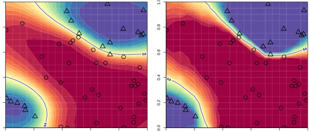
Figure 1: GPC model (3) based on EP and the logit function (left) and our GPC model (2) (right).
We now compare our model (2) with (3). The framework (2) corresponds to the limit of the model in (3), asσf →+∞. Indeed, let sgn(t) = 0 ift <0, sgn(t) = 1/2 ift= 0 and sgn(t) = 1
ift >0. Then, as observed in [22], whenσf = +∞, we haveP(I = 1|Zn, Z(x)) = sgn(Z(x))
and P(Ii = 1|Zn, Z(x)) = sgn(Z(xi)), for i = 1, . . . , n. Since the components of Zn take
values 0 with zero probability, (2) and (3) indeed give identical distributions of (I1, . . . , In, I)
whenσf = +∞.
In the framework described in Section 1, repeated calls to the code function for the same inputx either all crash or all successfully return an output value. Hence, model (2) is more appropriate than model (3) (especially with small values of σf). Figure 1 shows the two
models built on a 50 point design of experiments (obtained from the uniform distribution) on a 2D toy problem. While model (3), based on expectation-propagation (EP) [22], returns a function with smooth transitions, our model (2) returns a much sharper function, which is more appropriate for a framework of deterministic failures. In addition, model (3) returns conditional crash probabilities that are not equal to exactly zero or one for input points with observed binary outputs. By contrast, the conditional probabilities returned by our model (2) are exactly zero or one for these input points with observed outputs. Again this is more appropriate for deterministic failures.
In terms of inference, we have discussed in Section 2.1 that, for a fixedθ, the only costly step for model (2) is to sample realizations of the p.d.f. φZn
sn. This p.d.f. is that of a truncated
Gaussian vector (restricted to an orthant of Rn). Instead, the distribution to sample with
model (3) (the conditional distribution ofZn given I1 =i1, . . . , In=in) admits a density on Rn, which values atz1, . . . , zn are proportional to
n Y j=1 sig(σfzj)ij[1−sig(σfzj)]1−ij φZn(z1, . . . , zn), (4)
whereφZn is the Gaussian p.d.f. ofZ
n. The density in (4) is arguably more complicated than
as discussed above when introducing the references [4, 33, 23, 18].
In [26, 22], several approximations of the distribution in (4) by multidimensional Gaussian distributions are presented (in particular, the Laplace and EP approximations, the variational method and the Kullback-Leibler method). These approximations are usually relatively fast to obtain from local optimization methods. Yet, they are approximations of a non-Gaussian distribution, and do not come (to our knowledge) with theoretical guarantees. Similarly, for parameter estimation, the likelihood function ofI1, . . . , In is approximated, and the
approx-imation is maximized with respect to θ and σf. This yields a relatively fast procedure for
estimating θand σf, for which, again, no theoretical guarantees are available.
In contrast, with model (2), the simulation from the truncated conditional distribution
φZn
sn, with sn = (i1, . . . , in) (Section 2.1) and the maximum likelihood estimation of θ and µ
(Section 2.2) do not rely on approximations, and are based on Monte Carlo techniques rather than optimization. Hence, compared to model (3), the inference in model (2) may come with computational cost, but has more accuracy guarantees. For instance, there exists a large body of literature guaranteeing the convergence of Monte Carlo algorithms for long runs [20]. We assert that, with model (3) and the Gaussian approximation discussed above, once the conditional distribution of (Z(x1), . . . , Z(xn)) given I1 =i1, . . . , In = in is approximated, it
is not costly to obtain the conditional distribution ofI given (I1, . . . , In) (see [26, 22]). This
is similar to Algorithm 1 for model (2).
Finally, the constrained optimization problems addressed in the present article are of the form maxx∈Af(x), where A is a fixed unknown subset. It is hence very natural to use the
Bayesian prior{x∈ D;Z(x)>0} onA, which is obtained from our classification model (2). In contrast, classification model (3) does not provide a fixed set of admissible inputs, since any x in D has non-zero probabilities to yield both categories of the binary output. As a consequence, our suggested acquisition function in (9) below, and particularly its definition of the current admissible maximumMq, rely on classification model (2). Hence, also the proof
of convergence in Section 4 relies on classification model (2).
3
Bayesian optimization with crash constraints
Let us now address the case of optimization in the presence of computational failures. This problem requires a model for the objective function in addition to the one for the constraint. In this section, we first consider the problem of joint modeling, then its use in a Bayesian optimization algorithm.
3.1 Joint modeling of the objective and constraint
Let us consider two independent continuous Gaussian processes Y and Z from D to R. In
our framework, for an input pointx, we can observe the pair
(sign[Z(x)],sign[Z(x)]Y(x)). (5) That is, we observe whether the computation fails (Z(x) ≤0) or not, and in case of compu-tation success, we observe the objectiveY(x).
For Z, as in Section 2, we select a constant mean µZ ∈ R and a correlation parameter
θZ ∈ΘZ, where {kθZZ;θZ ∈ΘZ} is a set of correlation functions with ΘZ ⊂R
select a constant meanµY ∈Rand a covariance parameter θY ∈ΘY, where {kYθY;θY ∈ΘY}
is a set of covariance functions with ΘY ⊂RpY.
Let the pair (5) be observed for the input points x1, . . . , xn ∈ D. Forj = 1, . . . , nwe let
Ij = sign(Z(xj)) and consider the observation (i1, . . . , in, i1y1, . . . , inyn) of
(I1, . . . , In, I1Y(x1), . . . , InY(xn)). (6)
In the next lemma, we show that a likelihood can be defined for these 2n observations. Since the distribution of IiY(xi) is a mixture of continuous and discrete distributions, we
add a random continuous noise in case Ii = 0. This random noise does not add or remove
information, and is just a technicality in order to write the following lemma in terms of likelihood with respect to a simple fixed measure onR2n.
Let us introduce some notation before stating the lemma. For sn = (i1, . . . , in)> ∈ {0,1}n, letY
n,sn be the vector extracted from (Y(x1), . . . , Y(xn)) by keeping only the indices
j ∈ {1, . . . , n} for which ij = 1. Let φYµY,θ
Y,sn be the p.d.f. of Yn,sn, calculated under
the assumption thatY has a constant mean function µY and covariance function kθY
Y. For
v = (v1, . . . , vn)> ∈ Rn, let vsn be the vector extracted from v by keeping only the indices
j∈ {1, . . . , n}for which ij = 1.
Lemma 2. For j = 1, . . . , n, let Vj = IjY(xj) + (1 −Ij)Wj where W1, . . . , Wn are
in-dependent and follow the standard Gaussian distribution. Let fµZ,θ
Z,µY,θY be the p.d.f. of
(I1, . . . , In, V1, . . . , Vn), defined with respect to the measure (⊗ni=1µ)⊗(⊗ni=1λ) where µ is the counting measure on{0,1} and λis the Lebesgue measure on R. Then we have
fµZ,θ Z,µY,θY(i1, . . . , in, v1, . . . , vn) =PµZ,θ Z(I1=i1, . . . , In=in)φ Y µY,θ Y,sn(vsn) Y j=1,...,n ij=0 φ(vj) ,
whereφis the standard Gaussian p.d.f. andPµZ,θ
Z(·) is the probability of an event, calculated
under the assumption that Z has mean and covariance functions µZ and kθZ
Z.
Proof. The proof is deferred to Appendix A.
In view of Lemma 2, the maximum likelihood estimators ofµZ, θZ, µY, θY are
(ˆµZ,θˆZ)∈ argmax (µZ,θ Z)∈R×ΘZ PµZ,θ Z(I1 =i1, . . . , In=in) (7) and (ˆµY,θˆY)∈ argmax (µY,θ Y)∈R×ΘY φYµY,θ Y,sn(Yq), (8)
withYq the realization ofYn,sn.
The likelihood maximization in (7) can be tackled as in Section 2. The likelihood maxi-mization in (8) corresponds to the standard maximum likelihood in Gaussian process regres-sion.
Once the likelihood has been optimized, it is common practice to take the optimal mean and covariance parameters at face value and neglect the uncertainty associated with their esti-mation (the “plugin” approach), although more Bayesian alternatives have been proposed [3],
albeit at a higher computational cost. Note that, in practice, covariance parameters obtained from maximum likelihood estimation with data from deterministic functions can have unde-sirable properties in some cases. In particular, the estimates may depart substantially from oracle values (which would provide an efficient Gaussian process model for the deterministic function at hand) or even lead to failed runs in some cases [37]. In particular, overly large variance estimates may be obtained when working with the squared exponential covariance function [37]. For this reason, it is important to study the covariance parameter estimates that are obtained carefully, which we do in the numerical examples in Section 5. In addition, the squared exponential covariance function, leading to the potential issues described in [37], is not considered in Section 5; the Mat´ern covariance functions are considered instead.
Under the plugin approach, we provide the conditional distributions of Z and Y in the following lemma, given the observations in (6).
Lemma 3. Conditionally on
I1=i1, I1Y(x1) =i1y1, . . . , In=in, InY(xn) =inyn,
the stochastic processesY and Z are independent. The stochastic process Z follows the con-ditional distribution ofZ given I1 =i1, . . . , In =in and the stochastic process Y follows the
conditional distribution ofY given Yn,sn =Yq, with Yn,sn as in Lemma 2 and with Yq defined
as in (8).
Proof. The proof is deferred to Appendix A.
In other words, conditionally on the observations,Z is conditioned on its signs atx1, ..., xn,
andY is conditioned on its values at thexi’s for whichZ(xi)>0. Hence, conditional inference
on Z can be carried out as described in Section 2, and Y follows the standard Gaussian conditional distribution in Gaussian process regression.
3.2 Acquisition function and sequential design
Given the observations in (6), we now suggest an acquisition function that can be optimized to select a new observation pointxn+1∈ D, given a set of existing nobservations. We follow the classical improvement principle [21, 13], adapted to the partial observation setting. Thus, we choose: xn+1 ∈argmax x∈D E 1Z(x)>0[Y(x)−Mq]+ Fn , (9)
where (withσ(·) the sigma-algebra generated by a set of random variables):
Fn=σ(I1, I1Y(x1), . . . , In, InY(xn)) (10)
denotes our observation event and:
Mq= max
i=1,...,n;Z(xi)>0
Y(xi)
with the conventionMq =−∞ifZ(x1)≤0, . . . , Z(xn)≤0. We callE 1Z(x)>0[Y(x)−Mq]+
Fn
As in Lemma 3, forsn= (i1, . . . , in)∈ {0,1}n, we let Yn,sn be the vector extracted from
(Y(x1), . . . , Y(xn)) by keeping only the indices j ∈ {1, . . . , n} for which ij = 1. Thanks to
this lemma we have:
E 1Z(x)>0[Y(x)−Mq]+ Fn =P(Z(x)>0|I1=i1, . . . , In=in)E [Y(x)−Mq]+ Yn,sn :=Pnf(x)×EI(x). (11)
Hence, the EFI is equal to the product of the conditional probability of non-failure Pnf(x) (conditionally on the signs of Z) and of the standard expected improvement EI(x) (condi-tionally on the observed values ofY). This criterion is similar to the one proposed in [30] and later [6] for quantifiable constraints. The criterion in [17] is slightly different in order to favor the exploration of the boundary, but at the loss of a consistent definition of improvement:
EI(x)α1 × 2Pnf(x) (1−Pnf(x)) Pnf(x)−2wPnf(x) +w2 α2 ,
withα1, α1 andw positive parameters.
The conditional probability of non-failure Pnf(x) can be approximated by dPnf(x) from
Algorithm 1. In this algorithm, the first step is costly but needs to be performed only once independently of x, hence is outside the optimization loop (9). Then, dPnf(x) is a smooth
function of x that is not costly to evaluate.
Turning to the expected improvement EI(x), letqbe the length ofYn,sn. For a realization
(y1, . . . , yn) of (Y(x1), . . . , Y(xn)), let Yq be the vector extracted from (y1, . . . , yn) by keeping
only the indicesj ∈ {1, . . . , n}for which ij = 1. Hence,Yq is a realization of Yn,sn.
Letx→mYq(x, Yq) and (x, y)→kYq(x, y) be the conditional mean and covariance functions
ofY givenYn,sn =Yq. Let alsok
Y
q (x) =kYq(x, x). It is well-known (see e.g.[13]) that
EI(x) = mYq(x, Yq)−Mq Φ mYq(x, Yq)−Mq q kY q(x) + q kY q(x)φ mYq(x, Yq)−Mq q kY q(x) , (12)
with Φ andφthe c.d.f. and p.d.f. respectively of the standard Gaussian distribution.
Solving the optimization problem in (9) is greatly facilitated by analytical gradients, which are available in our case. Calculations are provided in Appendix C.
Remark 1. In the case of the global optimization of black box functions with statistical Bayesian models and in the absence of simulation failures, it is very common to select the observation points as maximizers of the expected improvement. Nevertheless, other ways of selecting the observation points exist, for instance maximizing the improvement probability (see (5) in [38]). In addition, [38] recently showed that the expected improvement strategy and the improvement probability are both special cases of a bi-objective optimization problem that consists in maximizing the conditional expectation (for a maximization problem) and the conditional variance as a function of the observation points.
In future work, it would be interesting to extend the improvement probability and the bi-objective setting to the case of simulation failures, as is done in (9) and (11) for the expected improvement. Our motivation for focusing on the expected improvement is its wide use in the absence of simulation failures and the fact that we obtain the expression (11)which is computationally convenient, in conjunction with Algorithm 1. Furthermore, convergence proofs exist for the optimization algorithm based on the expected improvement [34, 2], which we extend to the simulation failure case in the next section.
4
Convergence
In this section, we prove the convergence of the sequential choice of observation points given by (9), with the slight difference that (9) is replaced by
xn+1∈argmax x∈D E max u∈D P(Z(u)>0|Fn,x)=1 var(Y(u)|Fn,x)=0 Y(u)−M˜q Fn , (13) with ˜ Mq= max x∈D P(Z(x)>0|Fn)=1 kY q(x)=0 Y(x) (14)
and whereFn,x is the sigma algebra generated by the random variables
I1, I1Y(x1), . . . , In, InY(xn),1Z(x)>0,1Z(x)>0Y(x).
We note thatMq corresponds to the maximum over the q observed values ofY, while ˜Mq is
the maximum ofY over the input pointsxfor which it is known (after thenfirst observations) thatZ(x)>0 and that Y(x) =mYq(x, Yq).
The algorithms given by (9) and (13) coincide whenZ and Y are non-degenerate, that is
(ξ(vi))i=1,...,r has a non-degenerate distribution for any two-by-two distinct pointsv1, . . . , vr∈
D, withξ =Z andξ =Y. These two algorithms can be different whenY orZ are degenerate (which can happen, for instance, when their trajectories are known to satisfy symmetry properties, see e.g. [9]).
Hence, using (13) in the case of degenerate processes enables us to take into account that there are cases where some input points can be known to yield higher values ofY than maxYq
and to yield strictly positive values ofZ. Furthermore, (13) takes into account the fact that, foru6∈ {x1, . . . , xn, x}, the values1Z(u)>0 and Y(u) can have zero uncertainty when1Z(x)>0 and1Z(x)>0Y(x) are observed.
Following [34], we say that a Gaussian process ξ with continuous trajectories has the no-empty ball (NEB) property if, for anyx0 ∈ D and any >0,
inf
n∈N
x1,...,xn∈D
||xi−x0||≥,∀i
var(ξ(x0)|ξ(x1), . . . , ξ(xn))>0.
Many standard covariance kernels correspond to Gaussian processes having the NEB prop-erty. Indeed, a sufficient condition for the NEB property is that the covariance kernel is stationary with a spectral density decreasing no faster than an inverse polynomial at infin-ity [34]. The most notable covariance function that does not have the NEB property is the squared exponential covariance function [35], but other classical kernel families, such as the Mat´ern one used in our experiments, do.
We are now in position to state the convergence result.
Theorem 1. Let D be a compact hypercube of Rd. Let (Xi)i∈N be such thatX1=x1 is fixed in D and, forn≥1, Xn+1 is selected by (13).
θZ = 0.1 θZ= 0.3
θY = 0.1 case 1 case 3
θY = 0.3 case 2 case 4
Table 1: Studied ranges for the simulations.
1. Assume that Y and Z are Gaussian processes with continuous trajectories. Then, a.s. as n → ∞, supx∈DP(Z(x) > 0|Fn)(mYq(x, Yn,sn)−M˜q)
+ → 0 and sup
x∈DP(Z(x) >
0|Fn)kqY(x)→0.
2. Furthermore, if Y and Z have the NEB property, then (Xi)i∈N is a.s. dense in D. As
a consequence maxi=1,...,n;Z(Xi)>0Y(Xi)→maxu∈D;Z(u)>0Y(u) a.s. asn→ ∞.
Proof. Theorem 1 is proved by combining and extending the techniques from [34, 2]. The proof is deferred to Appendix A.
The first part of Theorem 1 states that, as n → ∞, all the input points x provide an asymptotically negligible expected improvement (similarly, a negligible information). Indeed, they either have a crash probability that goes to one, or a conditional variance that goes to zero and a conditional mean that is no larger than the current maximum ˜Mq.
The second part of the theorem shows that, as a consequence, the sequence of observation points is dense asn→ ∞and that the observed maximum converges to the global maximum. The nature of this convergence result is similar to those given in the unconstrained case in [34, 2]. This convergence result guarantees that our suggested algorithm will not leave unexplored regions. Another formulation of Theorem 1 is that our suggested algorithm will not be trapped in local maxima of Y.
5
Simulations on 2D Gaussian processes
In this section the behavior of our optimization algorithm with crash constraints, which we now call Expected Feasible Improvement with Gaussian Process Classification with signs (EFI GPC sign), is studied on simulated 2D Gaussian processes. We compare this algorithm with the optimization procedure defined in Section 3.2, but where the probabilities of satisfying the constraints are obtained from the classical Gaussian process classifier of [26, 22] based on Expectation Propagation; see Section 2.3. This second algorithm is called EFI GPC EP.
5.1 Simulations setting
The two algorithms are run on a function f : [0,1]2 → R taken as a realization of a 2D Gaussian process Y. The correlation kernel is a tensorized Matern5 2 kernel with the same correlation length parameter θY in each direction [27]. Observation of f is conditioned on a
functions : [0,1]2 → {0,1} such that s is a realization of 1Z>0, where Z is a 2D Gaussian process independent ofY. Z is also chosen with a tensorizedMatern5 2 kernel with the same parameter θZ in each direction.
Two levels of ranges forθY and θZ are considered to represent different behaviours of the
functions f and s. Four cases are studied and summarized in Table 1. In our simulations, the processes Y and Z have meanµY =µZ = 0 and variance σY2 =σ2Z= 1.
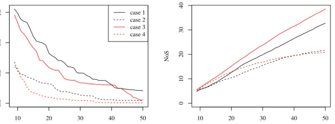
10 20 30 40 50 0.0 0.5 1.0 1.5 Number of simulations Rn case 1 case 2 case 3 case 4 10 20 30 40 50 0 10 20 30 40 Number of simulations NoS
Figure 2: Evolution of average Rn (left) and number of successes (NoS, right) along the
iteration steps. Four cases of range values are considered (see Table 1). Parameters are estimated by maximum likelihood.
The initial Design of Experiments (DoE) is a maximin Latin hypercube design of 9 points. Then, 41 points are sequentially added according to (15):
xn+1∈argmaxx∈DPnf(x)×EI(x). (15) Note that, as discussed above, Pnf(x) is calculated either through our algorithmGPC sign or by a classical GPC, which we denote as GPC EP.
5.2 Results of our method EFI GPC sign
In the following we define the regret at step n
Rn= max
x∈[0,1]2,Z(x)>0Y(x)−1≤i≤maxn,Z(x
i)>0
Y(xi).
It represents the gap between the global maximum and the current maximum value of the output on the current design of experiments{x1, . . . , xn}. We consider 20 different realizations
of Y and Z. In Figure 2 (left) the mean of Rn is plotted along the iteration steps in the
four different cases described in Table 1. It can be noticed that in each case the algorithm converges to the global maximum. The convergence speed depends on the range level. When the correlation length of the processY is high, i.e. θY = 0.3, the problem appears to be much
easier, independently of the correlation length of θZ. To a lesser extent, a high range of the
process Z also helps to accelerate the convergence.
The evolution of the Number of Successes (N oS) with iteration is plotted in Figure 2 (right). In case 2 and case 4 (θY = 0.3), the best point is rapidly found, exploration steps are then
more numerous and the increase ofN oS slows down.
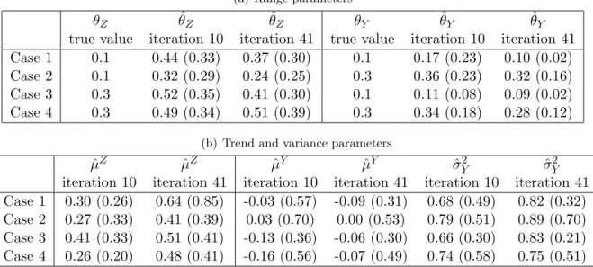
Range parameter estimations for the processesY andZ are given in the top table of Table 2. The bottom table gives the estimation of trend and variance parameters for both processes. It can be observed that parameter estimation for the process Z is difficult since only signs are available. For instance, µZ is overestimated. This reflects under-sampling of crash areas
that provide no information on the process Y. The situation is different for the process Y. Despite failure events, available information and estimation accuracy increase with iterations.
(a) Range parameters
θZ θˆZ θˆZ θY θˆY θˆY
true value iteration 10 iteration 41 true value iteration 10 iteration 41 Case 1 0.1 0.44 (0.33) 0.37 (0.30) 0.1 0.17 (0.23) 0.10 (0.02) Case 2 0.1 0.32 (0.29) 0.24 (0.25) 0.3 0.36 (0.23) 0.32 (0.16) Case 3 0.3 0.52 (0.35) 0.41 (0.30) 0.1 0.11 (0.08) 0.09 (0.02) Case 4 0.3 0.49 (0.34) 0.51 (0.39) 0.3 0.34 (0.18) 0.28 (0.12)
(b) Trend and variance parameters
ˆ
µZ µˆZ µˆY µˆY σˆY2 ˆσ2Y
iteration 10 iteration 41 iteration 10 iteration 41 iteration 10 iteration 41 Case 1 0.30 (0.26) 0.64 (0.85) -0.03 (0.57) -0.09 (0.31) 0.68 (0.49) 0.82 (0.32) Case 2 0.27 (0.33) 0.41 (0.39) 0.03 (0.70) 0.00 (0.53) 0.79 (0.51) 0.89 (0.70) Case 3 0.41 (0.33) 0.51 (0.41) -0.13 (0.36) -0.06 (0.30) 0.66 (0.30) 0.83 (0.21) Case 4 0.26 (0.20) 0.48 (0.41) -0.16 (0.56) -0.07 (0.49) 0.74 (0.58) 0.75 (0.51)
Table 2: MethodEFI GPC signat step 10 and 41: (a) Estimation ofθZandθY, (b) Estimation
ofµZ (true value is 0),µY (true value is 0) andσ2Y (true value is 1). Mean (standard deviation) over 20 simulations.
5.3 Comparison between EFI GPC sign and EFI GPC EP
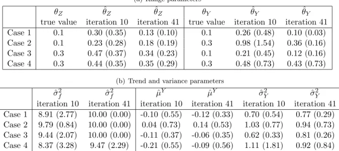
The performances of both methods (EFI GPC sign and EFI GPC EP) are compared on the same simulations as previously. It can be seen in Figure D.1 provided in Section D of the supplementary material that the regret of EFI GPC sign converges more rapidly to 0. This can be explained by the fact that the number of sucesses is more important with EFI GPC sign than with EFI GPC EP, since EFI GPC sign avoids crash areas more often (see Figure D.2 from the supplementary material). Parameter estimations of EFI GPC EP are given in Table 3. It can be observed that Z-parameter estimation can hardly be compared between methods since the classification models are different. Concerning the processY, the estimated correlation parameters tend towards the real values with more iterations. We note that when the estimated values of σf2 are large, the EP classification model is then close to the sign classification model.
An example of the progression of the algorithms in case 1 (θZ = θY = 0.1) is given in
Figures D.3 for EFI GPC sign and D.4 for EFI GPC EP in the supplementary material. Both algorithms evolve quite similarly butEFI GPC sign reaches the maximum a bit earlier. Moreover, the number of crashes is lower withEFI GPC sign than withEFI GPC EP.
6
Industrial case study
The aim of this section is to find the shape of an automotive fan system that maximizes its efficiency. The geometry of the turbomachinery (more precisely, that of the rotor blades) is described by 15 parameters: 5 chord lengths, 5 stagger angles and 5 heights of maximum camber. A drawing of a blade is provided in Figure E.1 in Section E in the supplementary material. A turbomachinery program has been developed by researchers at the LMFA (Lab-oratory of acoustics and fluid dynamics) in Ecole Centrale Lyon. It is a multi-physics 1D
(a) Range parameters
θZ θˆZ θˆZ θY θˆY θˆY
true value iteration 10 iteration 41 true value iteration 10 iteration 41 Case 1 0.1 0.30 (0.35) 0.13 (0.10) 0.1 0.26 (0.48) 0.10 (0.03) Case 2 0.1 0.23 (0.28) 0.18 (0.19) 0.3 0.98 (1.54) 0.36 (0.16) Case 3 0.3 0.47 (0.37) 0.34 (0.23) 0.1 0.21 (0.45) 0.12 (0.16) Case 4 0.3 0.44 (0.35) 0.35 (0.29) 0.3 0.48 (0.73) 0.43 (0.73)
(b) Trend and variance parameters
ˆ
σf2 σˆf2 µˆY µˆY ˆσY2 σˆ2Y
iteration 10 iteration 41 iteration 10 iteration 41 iteration 10 iteration 41 Case 1 8.91 (2.77) 10.00 (0.00) -0.10 (0.55) -0.12 (0.33) 0.70 (0.54) 0.77 (0.29) Case 2 9.79 (0.84) 10.00 (0.00) 0.04 (0.73) 0.14 (0.53) 1.03 (0.77) 0.94 (0.73) Case 3 9.44 (2.07) 10.00 (0.00) -0.11 (0.37) -0.06 (0.35) 0.62 (0.33) 0.81 (0.26) Case 4 8.37 (3.28) 9.47 (2.29) -0.21 (0.55) -0.09 (0.56) 1.11 (1.81) 0.92 (0.84)
Table 3: Mean and standard deviation (in parentheses) estimates (over 20 runs) of the kernel parameters at two steps of theEFI GPC EP method.
model based on iterative resolution of isentropic efficiency at medium radius, resolution of radial equilibrium, and deduction of blade angles through empirical correlations.
In this context we aim at selecting the geometric parameters that maximize the efficiency of the turbomachinery for a fixed input flow rate and for a fixed pressure rise. The ranges of the 15 geometric parameters are given in Table E.1 in the supplementary material.
For some parameter configurations the simulation does not converge and aNAis returned. These simulation failures can be related to the empirical rules injected in the implementation of the program, which limit its validity domain. Indeed, if the calculation comes out of the admissible domain, the empirical correlations become inaccurate and the simulation is not valid any more.
The issue is to find the optimal geometry considering these failures. A set of initial simulations has been run to explore failure events. We made each geometric parameter vary from its minimum to its maximum around three particular points on the diagonal of the hypercube in dimension 15;P oint1 is close to the minimal corner of the hypercube, P oint2 is at the center andP oint3 is close to the maximal corner of the hypercube. Coordinates are given in Table E.2 in the supplementary material.
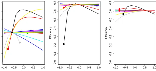
The results of these simulations are represented in Figure 3. It can be observed that
NAs are more frequent at the edges of the hypercube and near P oint1, although no obvious structure can be directly inferred. Besides, highest efficiencies are obtained around the center of the hypercube.
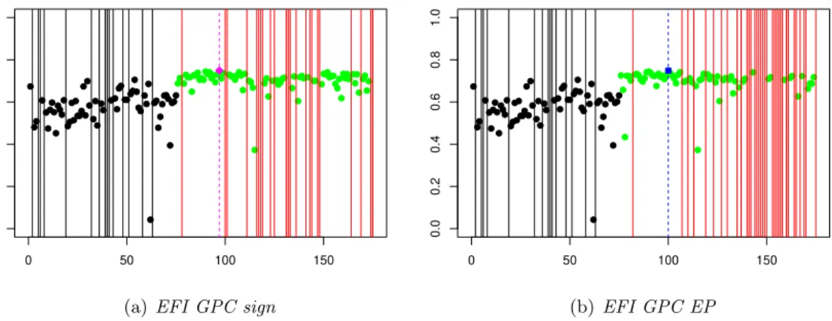
Both methodsEFI GPC sign andEFI GPC EP are applied from an initial maximin LHS composed of 75 points. Among them 18 simulations failed. The output range of the valid simulations is roughly [0.3,0.7] and the highest observed efficiency is 0.70. 100 simulations are then successively chosen according to (15). A tensorizedmatern5 2 kernel is chosen for both the Z and Y processes. As can be seen in Figure 4, a maximum efficiency of 0.75 is achieved at iteration 22 (resp. 25) for algorithmEFI GPC sign (resp. EFI GPC EP). Several types of behavior of the algorithms can be observed along the iterations. At the
−1.0 −0.5 0.0 0.5 1.0 0.0 0.1 0.2 0.3 0.4 0.5 0.6 0.7 a ) Point 1 Efficiency −1.0 −0.5 0.0 0.5 1.0 0.0 0.1 0.2 0.3 0.4 0.5 0.6 0.7 b ) Point 2 Efficiency −1.0 −0.5 0.0 0.5 1.0 0.0 0.1 0.2 0.3 0.4 0.5 0.6 0.7 c ) Point 3 Efficiency
Figure 3: Evolution of the efficiency (output of the code) from min to max in each direction around P oint1, P oint2 and P oint3. The colors indicate the different curves when varying the different input variables. A crash at a given value ofx is indicated by the absence of the curve value. The bullets are used to highlight the beginning of the crash ranges for the input variables. To simplify the reading, points are plotted in a normalized domain [−1,1]15.
beginning of the algorithms, simulations are added to locally improve efficiency; a single crash occurs over the 20 first points. Then, and especially above iteration 50, the algorithms explore other uncertainty areas and more failures occur. It can be noticed on Figure 4 that our algorithmEFI GPC sign avoids crash areas better than EFI GPC EP. Only 23 failures occur over 100 iterations withEFI GPC sign whereas 34 crashes occur with EFI GPC EP.
7
Conclusion
In this paper we have addressed the problem of global optimization of a black-box function under “crash” constraints. To do so, we revisited Gaussian process classification with a model based on observation signs. This model exhibited sharp classification boundaries, which were appropriate in our framework, and allowed us to propose the first algorithm with guaranteed convergence for this problem. Numerical experiments showed promising results, in particular as the algorithm causes fewer simulation failures (in a sense, wasted computational resources) that the current state-of-the-art.
For simplicity, we considered the case where simulations were run one at a time. A possible extension of this work would be to tackle the case of batch-sequential strategies, in the spirit of [8, 36]. We believe that both theoretical and practical aspects could be addressed without major difficulty. Another extension with practical importance would be to tackle problems for which either the objective function and/or the failure events are stochastic; however, a large portion of the proofs proposed here would not apply directly. Finally, convergence rates have not been considered here. Following [5, 32], future work may address this problem.
0 50 100 150 0.0 0.2 0.4 0.6 0.8 1.0 y
(a)EFI GPC sign
0 50 100 150 0.0 0.2 0.4 0.6 0.8 1.0 y (b) EFI GPC EP
Figure 4: Efficiency values for 175 geometric configurations. The first 75 points come from the initial DoE and are plotted in black. The 100 other points have been added by our optimization algorithms with failures (a)EFI GPC sign and (b)EFI GPC EP. Crashes are represented by vertical lines. On Figure (a) (resp. (b)), for EFI GPC sign (resp. EFI GPC EP), the best point is represented by a magenta diamond (resp. blue square) and is found at simulation number 97 (resp. 100).
Supplementary material
The supplementary material contains additional figures and tables for Sections 5 and 6.
Acknowledgments
This work was partly funded by the ANR project PEPITO. We are grateful to Jean-Marc Aza¨ıs and David Ginsbourger for discussing the topics in this paper.
A
Proofs
Proof of Lemma 1. With φZn the p.d.f. of Z
n and withsn= (i1, . . . , in)>, we have
Pnf(x) =P(Z(x)>0|sign(Zn) =sn) =E 1Z(x)>0 Qn j=11sign(Z(xj))=ij P(sign(Zn) =sn) = R Rnφ Zn(z 1, . . . , zn) Qn j=11sign(zj)=ij P(Z(x)>0|Z(x1) =z1, . . . , Z(xn) =zn)dz1. . . dzn P(sign(Zn) =sn) = Z Rn φZn sn(zn) ¯Φ −mZn(x, zn) p kZ n(x) ! dzn. (16)
The equation (16) is obtained by observing that
φZn(z 1, . . . , zn) Qn j=11sign(zj)=ij P(sign(Zn) =sn) = φ Zn(z 1, . . . , zn)1sign(Zn)=sn P(sign(Zn) =sn) =φZn sn(zn)
by definition ofφZn sn(zn), and that P(Z(x)>0|Z(x1) =z1, . . . , Z(xn) =zn) = ¯Φ −mZn(x, zn) p kZ n(x) ! by Gaussian conditioning.
Proof of Lemma 2. For any measurable function f, by the law of total expectation and using the independence ofY, (W1, . . . , Wn) andZ, we have
E[f(I1, . . . , In, V1, . . . , Vn)] = X i1,...,in∈{0,1} PµZ,θ Z(I1 =i1, . . . , In=in) E[f(i1, . . . , in, i1Y(x1) + (1−i1)W1, . . . , inY(xn) + (1−in)Wn)] = X i1,...,in∈{0,1} PµZ,θ Z(I1 =i1, . . . , In=in) Z Rn dvφYµY,θ Y,sn(vsn) Y j=1,...,n ij=0 φ(vj) f(i1, . . . , in, v1, . . . , vn).
This concludes the proof by definition of a p.d.f.
Proof of Lemma 3. Consider measurable functionsf(Y),g(Z),h(I1, . . . , In) andψ(I1Y(x1), . . . ,
InY(xn)). We have, by independence of Y and Z,
E[f(Y)g(Z)h(I1, . . . , In)ψ(I1Y(x1), . . . , InY(xn))] = X i1,...,in∈{0,1} P(I1=i1, . . . , In=in) E[f(Y)g(Z)h(i1, . . . , in)ψ(i1Y(x1), . . . , inY(xn))|I1 =i1, . . . , In=in] = X i1,...,in∈{0,1} P(I1=i1, . . . , In=in)h(i1, . . . , in) E[f(Y)ψ(i1Y(x1), . . . , inY(xn))]E[g(Z)|I1=i1, . . . , In=in] = X i1,...,in∈{0,1} P(I1=i1, . . . , In=in)h(i1, . . . , in) E[ψ(i1Y(x1), . . . , inY(xn))E[f(Y)|Yn,sn]]E[g(Z)|I1 =i1, . . . , In=in].
The last display can be written as, withLn the distribution of
I1, . . . , In, I1Y(x1), . . . , InY(xn),
Z
R2n
dLn(i1, . . . , in, i1y1, . . . , inyn)h(i1, . . . , in)ψ(i1y1, . . . , inyn) E[f(Y)|Yn,sn =Yq]E[g(Z)|I1=i1, . . . , In=in],
We now address the proof of Theorem 1. We let (Xi)i∈N be the random observation
points, such that Xi is obtained from (13) and (14) for i ∈ N. The next lemma shows
that conditioning on the random observation points and observed values works “as if” the observation pointsX1, . . . , Xn were non-random.
Lemma 4. For anyx1, . . . , xk∈ D,i1, ..., ik∈ {0,1}k and i1y1, ..., ikyk∈Rk, the conditional
distribution of(Y, Z) given
X1 =x1,sign(Z(X1)) =i1,sign(Z(X1))Y(X1) =i1y1, . . . ,
Xk=xk,sign(Z(Xk)) =ik,sign(Z(Xk))Y(Xk) =ikyk
is the same as the conditional distribution of(Y, Z) given
sign(Z(x1)) =i1,sign(Z(x1))Y(x1) =i1y1, . . . ,sign(Z(xk)) =ik,sign(Z(xk))Y(xk) =ikyk.
Proof. This lemma can be shown similarly as Proposition 2.6 in [2].
Proof of Theorem 1. Fork∈N, we remark thatFk is the sigma-algebra generated by
X1,sign(Z(X1)),sign(Z(X1))Y(X1), . . . , Xk,sign(Z(Xk)),sign(Z(Xk))Y(Xk).
We let Ek, Pk and vark denote the expectation, probability and variance conditionally on Fk. Forx ∈ D, we let Ek,x,Pk,x and vark,x denote the expectation, probability and variance
conditionally on
X1,sign(Z(X1)),sign(Z(X1))Y(x1), . . . , Xk,sign(Z(Xk)),sign(Z(Xk))Y(Xk), x,sign(Z(x)),sign(Z(x))Y(x).
We let σ2k(u) = vark(Y(u)), mk(u) = Ek[Y(u)] and Pk(u) = Pk(Z(u) > 0). We also let
σ2k,x(u) = vark,x(Y(u)), mk,x(u) =Ek,x[Y(u)] andPk,x(u) =Pk,x(Z(u)>0).
With these notations, the observation points satisfy, fork∈N,
Xk+1 ∈argmaxx∈DEk max u:Pk,x(u)=1 σk,x(u)=0 Y(u)−Mk , (17) where Mk= max u:Pk(u)=1 σk(u)=0 Y(u).
We first show that (17) can be defined as a stepwise uncertainty reduction (SUR) sequential design [2]. We have Xk+1∈argmaxx∈DEk P max k,x(u)=1 σk,x(u)=0 Y(u)− max Pk(u)=1 σk(u)=0 Y(u) (18) ∈argminx∈DEk Ek,x max Z(u)>0Y(u) − max Pk,x(u)=1 σk,x(u)=0 Y(u)
since the second term in (18) does not depend on x and from the law of total expectation. We let Hk=Ek Zmax(u)>0Y(u)−Pmax k(u)=1 σk(u)=0 Y(u) and Hk,x=Ek,x Zmax(u)>0Y(u)−P max k,x(u)=1 σk,x(u)=0 Y(u) .
Then we have fork≥1
Xk+1 ∈argminx∈DEk(Hk,x).
We have, using the law of total expectation, and since Ek,x
h maxPk,x(u)=1,σk,x(u)=0Y(u) i = maxPk,x(u)=1,σk,x(u)=0Y(u), Hk−Ek(Hk+1) =Ek max Pk,Xk +1(u)=1 σk,Xk +1(u)=0 Y(u)− max Pk(u)=1 σk(u)=0 Y(u) ≥0
since, for allu, x∈ D,σk,x(u)≤σk(u) andPk(u) = 1 impliesPk,x(u) = 1. Hence (Hk)k∈Nis a supermartingale and of courseHk≥0 for allk∈N. Also|H1| ≤2E1[maxu∈D|Y(u)|] so that H1 is bounded inL1, since the mean value of the maximum of a continuous Gaussian process on a compact set is finite. Hence, from Theorem 6.23 in [14],Hkconverges a.s. ask→ ∞to a
finite random variable. Hence, as in the proof of Theorem 3.10 in [2], we have Hk−Ek(Hk+1)
goes to 0 a.s. as k→ ∞. Hence, by definition ofXk+1we obtain supx∈D(Hk−Ek(Hk,x))→0
a.s. as k→ ∞. This yields, from the law of total expectation,
0←−a.s.n→∞sup x∈DEk max Pk,x(u)=1 σk,x(u)=0 Y(u)− max Pk(u)=1 σk(u)=0 Y(u) (19) ≥sup x∈DEk 1Z(x)>0(Y(x)−Mk)+ ≥sup x∈D Pk(x)γ(mk(x)−Mk, σk(x)),
from Lemma 3 and (12), where
γ(a, b) =aΦa b +bφa b .
Recall from Section 3 in [34] that γ is continuous and satisfies γ(a, b) > 0 if b > 0 and
γ(a, b) ≥aif a >0. We have fork∈N, 0≤σk(u) ≤maxv∈D
p
var(Y(v))<∞. Also, with the same proof as that of Proposition 2.9 in [2], we can show that the sequence of random functions (mk)k∈Nconverges a.s. uniformly onDto a continuous random functionm∞onD. Thus, from (19), by compacity, we have, a.s. as k → ∞, supx∈DPk(x)(mk(x)−Mk)+ → 0
Let us address Part 2. For all τ ∈ N, consider fixed v1, . . . , vNτ ∈ D for which maxu∈D
mini=1,...,Nτ ||u−vi|| ≤ 1/τ. Consider the event Eτ = {∃u ∈ D; infi∈N||Xi −u|| ≥ 2/τ}.
Then,Eτ implies the event Ev,τ =∪jN=1τ Ev,τ,j whereEv,τ,j ={infi∈N||Xi−vj|| ≥1/τ}. Let
us now show that P(Ev,τ,j) = 0 for j = 1, . . . , Nτ. Assume thatEv,τ,j ∩ C holds, where C is
the event in Part 1. of the theorem, withP(C) = 1. Since Y has the NEB property, we have
lim infk→∞σk(vj)>0. Hence,Pk(vj)→0 as k→ ∞ sinceC is assumed. We then have
var(1Z(vj)>0|1Z(X1)>0, . . . ,1Z(Xk)>0) =Pk(vj)(1−Pk(vj))→0 (20)
a.s. ask→ ∞. But we have
var(1Z(vj)>0|1Z(X1)>0, . . . ,1Z(Xk)>0) =E 1Z(vj)>0−Pk(vj) 2 1Z(X1)>0, . . . ,1Z(Xk)>0 =E E 1Z(vj)>0−Pk(vj) 2 Z(x1), . . . , Z(xk) 1Z(X1)>0, . . . ,1Z(Xk)>0 .
SincePk(vj) is a function of Z(x1), . . . , Z(xn), we obtain
var(1Z(vj)>0|1Z(X1)>0, . . . ,1Z(Xk)>0) ≥Ehvar1Z(vj)>0|Z(x1), . . . , Z(xk) 1Z(X1)>0, . . . ,1Z(Xk)>0 i =E g ¯ Φ − mk(vj) σk(vj) 1Z(X1)>0, . . . ,1Z(Xk)>0 ,
with g(t) = t(1−t) and with ¯Φ as in Lemma 1. We let S = supk∈N|mk(vj)| and s =
infk∈Nσk(vj). Then, from the uniform convergence ofmk discussed below and from the NEB
property ofZ, we haveP(ES,s) = 1 where ES,s={S <+∞, s >0}. Then, ifEv,τ,j∩ C ∩ES,s
holds, we have var(1Z(vj)>0|1Z(X1)>0, . . . ,1Z(Xk)>0) ≥E g ¯ Φ S s 1Z(X1)>0, . . . ,1Z(Xk)>0 →a.s.k→∞E g ¯ Φ S s FZ,∞ , whereFZ,∞=σ(
1Z(Xi)>0) i∈N) from Theorem 6.23 in [14]. Almost surely, conditionally on FZ,∞ we have a.s. S < ∞ and s > 0. Hence we obtain that, on the event Ev,τ,j ∩ A with P(A) = 1, var(1Z(vj)>0|1Z(X1)>0, . . . ,1Z(Xk)>0) does not go to zero. Hence, from (20), we
haveP(Ev,τ,j) = 0. This yields that (Xi)i∈N is a.s. dense inD. Hence, since{u;Z(u)>0} is
an open set, we have maxi;Z(Xi)>0Y(Xi)→maxZ(u)>0Y(u) a.s. as n→ ∞.
B
Stochastic approximation of the likelihood gradient for
Gaus-sian process based classification
In Appendixes B and C, for two matricesAandB of sizesa×dandb×d, and for a function
h:Rd×Rd→R, leth(A, B) be thea×bmatrix [h(ai, bj)]i=1,...,a,j=1,...,b, whereai andbj are
Let sn = (i1, . . . , in) ∈ {0,1}n be fixed. Assume that the likelihood Pµ,θ(sign(Zn) = sn)
has been evaluated by ˆPµ,θ(sign(Zn) = sn). Assume also that realizations zn(1), . . . , z(nN),
approximately following the conditional distribution ofZn given sign(Zn) =sn, are available.
LetZ ={zn∈Rn : sign(zn) =sn}. Treatingx1, . . . , xn asd-dimensional line vectors, let
xbe the matrix (x>1, . . . , x>n)>. Then we have
Pµ,θ(sign(Zn) =sn) = Z Z 1 (2π)n/2 1 q |kθZ(x,x)| e−21(zn−µ1n) >kZ θ(x,x) −1(z n−µ1n)dz n,
where 1n= (1, . . . ,1)>∈Rn and |.|denotes the determinant.
Derivating with respect toµ yields
∂ ∂µPµ,θ(sign(Zn) =sn) = Z Z 1 (2π)n/2 1 q |kθZ(x,x)| e−21(zn−µ1n) >kZ θ(x,x) −1(z n−µ1n) (1>nkθZ(x,x)−1(zn−µ1n))dzn =Pµ,θ(sign(Zn) =sn)Eµ,θ 1>nkZθ(x,x)−1(Zn−µ1n) sign(Zn) =sn) ,
where Eµ,θ means that the conditional expectation is calculated under the assumption that
Z has constant mean function µand covariance function kθZ. Hence we have the stochastic approximation ˆ∇µ for∂/∂µPµ,θ(sign(Zn) =sn) given by
ˆ ∇µ= ˆPµ,θ(sign(Zn) =sn) 1 N N X i=1 1>nkθZ(x,x)−1(z(ni)−µ1n).
Derivating with respect toθi fori= 1, . . . , pyields, with adj(M) the adjugate of a matrixM,
∂ ∂θiPµ,θ (sign(Zn) =sn) = Z Z − 1 2 |k Z θ(x,x)| −1Tr adj(kθZ(x,x))∂k Z θ(x,x) ∂θi +1 2(zn−µ1n) >∂kθZ(x,x) ∂θi kθZ(x,x)−1∂k Z θ(x,x) ∂θi (zn−µ1n) 1 (2π)n/2 1 q |kZ θ(x,x)| e−21(zn−µ1n) >kZ θ(x,x) −1(z n−µ1n)dz n =Pµ,θ(sign(Zn) =sn) Eµ,θ −1 2 |k Z θ(x,x)| −1Tr adj(kZθ(x,x))∂k Z θ(x,x) ∂θi +1 2(Zn−µ1n) >∂kZθ(x,x) ∂θi kZθ(x,x)−1∂k Z θ(x,x) ∂θi (Zn−µ1n) sign(Zn) =sn) .
Hence we have the stochastic approximation ˆ∇θi for∂/∂θiPµ,θ(sign(Zn) =sn) given by
ˆ ∇θi = ˆPµ,θ(sign(Zn) =sn) 1 N N X i=1 − 1 2 |k Z θ(x,x)|−1Tr adj(kZθ(x,x))∂k Z θ(x,x) ∂θi +1 2(z (i) n −µ1n)> ∂kZθ(x,x) ∂θi kθZ(x,x)−1∂k Z θ(x,x) ∂θi (zn(i)−µ1n) .
Remark 2. Several implementations of algorithms are available to obtain the realizations
zn(1), . . . , zn(N), as discussed after Algorithm 1. It may also be the case that some
implementa-tions provide both the estimate Pˆµ,θ(sign(Zn) =sn) and the realizations zn(1), . . . , zn(N).
C
Expressions of the mean and covariance of the conditional
Gaussian process and of the gradient of the acquisition
function
Let µY and kY be the mean and covariance functions of Y. Treating x1, . . . , xn as d
-dimensional line vectors, letxq be the matrix extracted from (x>1, . . . , x>n)> by keeping only
the lines which indicesj satisfyij = 1.
We first recall the classical expressions of GP conditioning:
mYq(x, Yq) = µY +kY(x,xq) kY(xq,xq) −1 Yq−µY kYq(x, x0) = kY(x, x0)−kY(x,xq) kY(xq,xq) −1 kY(xq, x0).
∇xmYq(x, Yq) and∇xkqY(x, x) are straightforward provided that∇xkY(x, y) is available: ∇xmYq(x, Yq) = [∇xkY(x,xq)] kY(xq,xq) −1 Yq−µY ∇xkqY(x, x) = ∇xkY(x, x)−2kY(x,xq) kY(xq,xq) −1 ∇xkY(xq, x). Then: ∇xEIq(x) = Φ mYq(x, Yq)−Mq q kY q(x, x) ∇xmYq(x, Yq)+φ Mq−mYq(x, Yq) q kY q (x, x) 1 2 q kY q (x, x) ∇xkqY(x, x).
For Pnf(x), using the approximation of Algorithm 1, we have:
d Pnf(x) = 1 N N X i=1 ¯ Φ −m Z n(x, z (i) n ) p kZ n(x, x) ! , with knZ(x, x) as kYn(x, x) and mZn(x, zn(i)) =µZ+kZ(x,x) kZ(x,x)−1 z(ni)−µZ.
Applying the standard differentiation rules delivers:
∇xdPnf(x) = 1 N N X i=1 φ m Z n(x, z (i) n ) p kZ n(x, x) ! " 1 p kZ n(x, x) ∇xmZn(x, zn(i))− m Z n(x, z (i) n ) 2[kZ n(x, x)]3/2 ∇xkZn(x, x) # .
References
[1] D. Azzimonti and D. Ginsbourger. Estimating orthant probabilities of high-dimensional Gaussian vectors with an application to set estimation. Journal of Computational and Graphical Statistics, 27(2):255–267, 2018.
[2] J. Bect, F. Bachoc, and D. Ginsbourger. A supermartingale approach to Gaussian process based sequential design of experiments. Bernoulli, 25(4A):2883–2919, 2019.
[3] R. Benassi, J. Bect, and E. Vazquez. Robust Gaussian process-based global optimization using a fully Bayesian expected improvement criterion. In International Conference on Learning and Intelligent Optimization, pages 176–190. Springer, 2011.
[4] Z. I. Botev. The normal law under linear restrictions: simulation and estimation via min-imax tilting. Journal of the Royal Statistical Society: Series B (Statistical Methodology), 79(1):125–148, 2017.
[5] A. D. Bull. Convergence rates of efficient global optimization algorithms. Journal of Machine Learning Research, 12(Oct):2879–2904, 2011.
[6] M. A. Gelbart, J. Snoek, and R. P. Adams. Bayesian optimization with unknown con-straints. In UAI, 2014.
[7] A. Genz. Numerical computation of multivariate normal probabilities. Journal of com-putational and graphical statistics, 1(2):141–149, 1992.
[8] D. Ginsbourger, R. Le Riche, and L. Carraro. Kriging is well-suited to parallelize opti-mization. In Computational intelligence in expensive optimization problems, pages 131– 162. Springer, 2010.
[9] D. Ginsbourger, O. Roustant, and N. Durrande. On degeneracy and invariances of ran-dom fields paths with applications in Gaussian process modelling. Journal of statistical planning and inference, 170:117–128, 2016.
[10] R. Gramacy and H. Lee. Optimization under unknown constraints. Bayesian Statistics, 9, 2011.
[11] R. B. Gramacy, G. A. Gray, S. Le Digabel, H. K. Lee, P. Ranjan, G. Wells, and S. M. Wild. Modeling an augmented Lagrangian for blackbox constrained optimization. Tech-nometrics, 58(1):1–11, 2016.
[12] J. M. Hernandez-Lobato, M. Gelbart, M. Hoffman, R. Adams, and Z. Ghahramani. Predictive entropy search for Bayesian optimization with unknown constraints. In Inter-national Conference on Machine Learning, pages 1699–1707, 2015.
[13] D. Jones, M. Schonlau, and W. Welch. Efficient global optimization of expensive black box functions. Journal of Global Optimization, 13:455–492, 1998.
[14] O. Kallenberg. Foundations of Modern Probability. Second edition. Springer-Verlag, 2002.
[15] K. Kandasamy, W. Neiswanger, J. Schneider, B. Poczos, and E. P. Xing. Neural archi-tecture search with Bayesian optimisation and optimal transport. InAdvances in Neural Information Processing Systems, pages 2016–2025, 2018.
[16] A. Keane and P. Nair. Computational approaches for aerospace design: the pursuit of excellence. John Wiley & Sons, 2005.
[17] D. V. Lindberg and H. K. Lee. Optimization under constraints by applying an asymmetric entropy measure. Journal of Computational and Graphical Statistics, 24(2):379–393, 2015.
[18] A. F. L´opez-Lopera, F. Bachoc, N. Durrande, and O. Roustant. Finite-dimensional Gaussian approximation with linear inequality constraints. SIAM/ASA Journal on Un-certainty Quantification, 6(3):1224–1255, 2018.
[19] H. Maatouk and X. Bay. A New Rejection Sampling Method for Truncated Multivari-ate Gaussian Random Variables Restricted to Convex Sets, pages 521–530. Springer International Publishing, Cham, 2016.
[20] S. P. Meyn and R. L. Tweedie. Markov chains and stochastic stability. Springer Science & Business Media, 2012.
[21] J. B. Mockus, V. Tiesis, and A. ˇZilinskas. The application of Bayesian methods for seeking the extremum. In L. C. W. Dixon and G. P. Szeg¨o, editors, Towards Global Optimization, volume 2, pages 117–129, North Holland, New York, 1978.
[22] H. Nickisch and C. E. Rasmussen. Approximations for binary Gaussian process classifi-cation. Journal of Machine Learning Research, 9(Oct):2035–2078, 2008.
[23] A. Pakman and L. Paninski. Exact Hamiltonian Monte Carlo for truncated multivariate Gaussians. Journal of Computational and Graphical Statistics, 23(2):518–542, 2014. [24] V. Picheny. A stepwise uncertainty reduction approach to constrained global
optimiza-tion. In Artificial Intelligence and Statistics, pages 787–795, 2014.
[25] V. Picheny, R. B. Gramacy, S. Wild, and S. Le Digabel. Bayesian optimization under mixed constraints with a slack-variable augmented Lagrangian. In Advances in Neural Information Processing Systems, pages 1435–1443, 2016.
[26] C. Rasmussen and C. Williams. Gaussian Processes for Machine Learning. The MIT Press, Cambridge, 2006.
[27] O. Roustant, D. Ginsbourger, and Y. Deville. DiceKriging, DiceOptim: Two R packages for the analysis of computer experiments by Kriging-based metamodeling and optimiza-tion. Journal of statistical software, 51(1):1–55, 2012.
[28] M. Sacher, R. Duvigneau, O. Le Maitre, M. Durand, E. Berrini, F. Hauville, and J.-A. Astolfi. A classification approach to efficient global optimization in presence of non-computable domains. Structural and Multidisciplinary Optimization, 58(4):1537–1557, 2018.
[29] M. J. Sasena, P. Papalambros, and P. Goovaerts. Exploration of metamodeling sampling criteria for constrained global optimization. Engineering optimization, 34(3):263–278, 2002.
[30] M. Schonlau, W. J. Welch, and D. R. Jones. Global versus local search in constrained optimization of computer models. Lecture Notes-Monograph Series, pages 11–25, 1998. [31] J. Snoek, H. Larochelle, and R. P. Adams. Practical Bayesian optimization of machine
learning algorithms. InAdvances in neural information processing systems, pages 2951– 2959, 2012.
[32] N. Srinivas, A. Krause, S. Kakade, and M. Seeger. Gaussian process optimization in the bandit setting: no regret and experimental design. In Proceedings of the 27th Interna-tional Conference on Machine Learning, pages 1015–1022, 2010.
[33] J. Taylor and Y. Benjamini. RestrictedMVN: multivariate normal restricted by affine con-straints. https://cran.r-project.org/web/packages/restrictedMVN/index.html, 2017. [Online; 02-Feb-2017].
[34] E. Vazquez and J. Bect. Convergence properties of the expected improvement algorithm with fixed mean and covariance functions. Journal of Statistical Planning and inference, 140(11):3088–3095, 2010.
[35] E. Vazquez and J. Bect. Pointwise consistency of the kriging predictor with known mean and covariance functions. InmODa 9–Advances in Model-Oriented Design and Analysis, pages 221–228. Springer, 2010.
[36] J. Wu and P. Frazier. The parallel knowledge gradient method for batch Bayesian op-timization. In Advances in Neural Information Processing Systems, pages 3126–3134, 2016.
[37] A. Zhigljavsky and A. ˇZilinskas. Selection of a covariance function for a Gaussian random field aimed for modeling global optimization problems. Optimization Letters, 13(2):249– 259, 2019.
[38] A. ˇZilinskas and J. Calvin. Bi-objective decision making in global optimization based on statistical models. Journal of Global Optimization, 74(4):599–609, 2019.