sciences
ArticleAdaptive Dynamic Disturbance Strategy for
Di
ff
erential Evolution Algorithm
Tiejun Wang1,* , Kaijun Wu2 , Tiaotiao Du2and Xiaochun Cheng3,*
1 School of Mathematics and Computer Science Institute, Northwest Minzu University, LanZhou 730030, China
2 School of Electronic and Information Engineering, LanZhou Jiao Tong University, LanZhou 730070, China; [email protected] (K.W.); [email protected] (T.D.)
3 Department of Computer Science, Middlesex University, London NW4 4BT, UK * Correspondence: [email protected] (T.W.); [email protected] (X.C.)
Received: 22 February 2020; Accepted: 9 March 2020; Published: 13 March 2020
Abstract: To overcome the problems of slow convergence speed, premature convergence leading to local optimization and parameter constraints when solving high-dimensional multi-modal optimization problems, an adaptive dynamic disturbance strategy for differential evolution algorithm (ADDSDE) is proposed. Firstly, this entails using the chaos mapping strategy to initialize the population to increase population diversity, and secondly, a new weighted mutation operator is designed to weigh and combinemutation strategies of the standard differential evolution (DE). The scaling factor and crossover probability are adaptively adjusted to dynamically balance the global search ability and local exploration ability. Finally, a Gauss perturbation operator is introduced to generate a random disturbance variation, and to accelerate premature individuals to jump out of local optimization. The algorithm runs independently on five benchmark functions 20 times, and the results show that the ADDSDE algorithm has better global optimization search ability, faster convergence speed and higher accuracy and stability compared with other optimization algorithms, which provide assistance insolving high-dimensionaland complex problems in engineering and information science.
Keywords: differential evolution algorithm; adaptive dynamic disturbance strategy; Gauss perturbation; benchmark functions
1. Introduction
The differential evolution (DE) algorithm was proposed by Storn and Price in 1995 [1,2]. It was originally used to solve the Chebyshev polynomial problem, and is a bionic optimization algorithm based on swarm evolution. DE’s unique population memory capability gives the algorithm a strong global search capability and robust performance. As a highly efficient parallel search algorithm with few controlled parameters, the DE algorithm has been widely used in neuron networks [3,4], power systems [5,6], vehicle routing problems [7–11] and many other fields [12–20]. Like other intelligent algorithms, however, the DE algorithm also has disadvantages such as precocity, strong parameter dependence and difficulty in obtaining global optimum values for high-dimensional complex objective functions [21–27]. Therefore, researchers proposed a number of improvement strategies for DE’s existing shortcomings. First, to improve the existing parameters—Chiou et al. [28] proposed a variable scaling factor differential evolution algorithm, which does not require mutation selection. The type of operation, compared to the random scaling factor, has a large improvement in performance. Secondly, adding new operations was suggested—Wang et al. [29] proposed a generalized inverse differential evolution algorithm, which introduces generalized opposition-based learning based on
reverse learning techniques; this prevents the algorithm from falling into a local optimum to a certain extent. Third, multiple groups—Ali et al. [30] divided the population into independent subgroups, with each having different mutation and updating strategies, and introduced a multi-population DE to solve large-scale global optimization problems. Finally, the fourth suggestion was the hybrid algorithm—Trivedi et al. [31] proposed a hybrid evolutionary model based on genetic algorithms and differential evolution. The binary variables evolved based on the genetic algorithm and the continuous variables evolved based on the DE algorithm, which was used to solve a nonlinear, high-dimensional, highconstrained and mixed-integeroptimization problem.
These classical improved algorithms improve the optimization performance of the DE algorithm to a certain extent, but for some high-dimensional and complex problems, there are still disadvantages of falling into the local optimum. Experiments show that the most critical operation in the DE algorithm is differential variation, and the core of differential variation is the composition of differential vectors. Most of the existing improved algorithms adopt adaptive adjustment parameters or randomly choose a mutation strategy. Although the random strategy improves the global search ability of the algorithm and population diversity, the evolutionary direction of the population is more difficult to control, which may cause the population to deviate from the direction of the optimal value search, and an excessive number of iterations will also lead to a decrease in the convergence rate of the algorithm.
In order to balance the global optimum and the local optimum, an adaptive dynamic disturbance strategy differential evolution algorithm is proposed in this paper. On the basis of the adaptive adjustment of policy level control parameters, it is added a dimensional variation disturbance strategy. Through the theoretical analysis of algorithm factors and performance testing of standard test functions, the results show that when the adaptive dynamic disturbance strategy for differential evolution (ADDSDE) algorithm is used to solve complex optimization problems such as high-dimensions and multi-peaks, the global optimal solution can be obtained with a minimum number of iterations, and the algorithm has strong robustness.
2. Standard Differential Evolution Algorithms
The differential evolution (DE) algorithm is a group heuristic optimization algorithm based on real coding. Its basic idea is to dynamically search the global optimal value through information sharing between groups and the unique memory of each individual. The main operations include mutation, crossover and selection. According to the loop iterations of mutation, crossover and selection operations, the population continuously evolves towards the optimal value. The specific definition is as follows:
Each population in the DE algorithm consists of N individuals, and is expressed as: X = [x1,x2,. . .,xN], whereNis the number of populations; each individual corresponds to the solution of the problem to be solved, expressed as: xi(g) = (xi1(g),xi2(g),. . .,xiD(g)), whereDis the dimension of solution,xi j(g)is the j-th component of thei-th evolving individual in the g-th generation of the population.
2.1. Initialization
The DE algorithm initializes the population according to the principle of randomness, and sets the optimization interval for variables as[xmin,xmax]. The initialization operation is defined as follows xi j(0) =xmin,j+rand()·(xmax,j−xmin.j) (1) whererand()is a random number uniformly distributed in the interval [0,1].
2.2. Mutation Operation
In each generation of evolution, the DE algorithm generates variant individuals for each individual xi j(g)in the population, based on the mutation operation. Currently, there are multiple versions of the
variants, which are expressed asDE/a/b, and among them,ais the type of the mutation operator, which is generally valued asrandandbest:randmeans randomly selecting an individual from the population as the mutation base, andbestrepresents selecting the optimal individual from the population as the mutation base; whilebrepresents the number of differential terms, which is generally an integer. Common mutation operation schemes are as follows:
DE/rand/1: ti,j(g) =xr1,j(g) +F·[xr2,j(g)−xr3,j(g)] (2) DE/best/1: ti,j(g) =xbest(g) +F·[xr1,j(g)−xr2,j(g)] (3) DE/rand/2: ti,j(g) =xr1,j(g) +F·[xr2,j(g)−xr3,j(g)] +F·[xr4,j(g)−xr5,j(g)] (4) DE/best/2: ti,j(g) =xbest(g) +F·[xr1,j(g)−xr2,j(g)] +F·[xr3,j(g)−xr4,j(g)] (5) Among these,r1,r2,r3,r4,r5,i∈ {1, 2,. . .,N}, andr1,r2,r3,r4,r5,i, Niis the number of populations,xbest(g)is the optimal individual of theg-th generation andFis the scaling factor. 2.3. Crossover Operation
In order to increase the diversity of the population, the DE algorithm cross-processes the original individualxi j(g)with the generated variant individualti j(g)according to the crossover probability CR, thereby generating a new variant individualvi j(g). Common crossovers have two crosses, defined as follows: vi j(g) = ti j(g) rand<CR or j=r xi j(g) otherwise (6)
Among these:randis the random number that is uniformly distributed in the interval [0,1],CRis the crossover probability andris the random integer in the interval[1, 2,. . .,D].
2.4. Selection Operation
In order to determine which individual evolved to adopt the greedy choice method for the next-generation DE algorithm—that is, to compare the fitness function values of the mutant individual vi j(g)with the original individualxi j(g)—the individual with higher fitness value is selected to enter the next generation. The definition is as follows:
xi j(g+1) = vi j(g) f[vi j(g)]< f[xi j(g)] xi j(g) otherwise (7)
Among these: f(x)is the fitness function or objective function.
3. An adaptive Dynamic Disturbance Strategy for Differential Evolution Algorithm
The core idea of an improved differential evolution (DE) algorithm is to generate variation disturbance according to vector difference, ensure the diversity of the population, balance global search and local development ability, avoid precocity of population, accelerate the rate of population convergence and improve the convergence accuracy. So, the adaptive dynamic disturbance strategy for differential evolution (ADDSDE) algorithm mainly improves the algorithm from four aspects of population initialization, parameter adaptation, mutation strategy and disturbance strategy, and comprehensively improves the global optimization search ability and convergence speed of the
algorithm. Firstly, the chaos mapping theory is used to initialize the population. The standard DE algorithm is a random initialization population. Although it is beneficial to the diversity of population, it is difficult to guarantee that the quality of the population individual and the efficiency of the algorithm is reduced. Second, an adaptive adjustment mechanism for scaling factor F and crossover probability CR is adopted to improve the convergence speed and stability of the algorithm. Third, the mutation strategiesDE/rand/1 andDE/best/1 are dynamically weighted, and balance the global search and local search. Finally, the Gauss perturbation strategy is introduced to accelerate individuals to jump out of the local optimum and improve the global search ability.
3.1. Population Initialization of Chaotic Maps
The initial population of the standard DE algorithm is randomly generated. The initial population may gather in a certain area that deviates from the optimal value, thereby reducing the efficiency of the algorithm. Chaos is a stochastic phenomenon generated by a deterministic nonlinear dynamical system. It has the characteristics of equilibrium instability and mutation. It can go through all states within a certain range without repetition—that is, the randomness, regularity and ergodicity of chaos. The most commonly used chaotic model is a one-dimensional Logistic nonlinear mapping [32], and its optimization formula is:
yk+1=µyk(1−yk) (8)
In this formula,µis the control parameter whose value is a normal number, andk=0, 1, 2. . . is the number of iterations. When the value ofµis determined, given the initial valuey0∈(0, 1), the population sequencey1,y2,. . .ykis obtained after several iterations. According to experience, when µ=4, the system presents full chaos phenomenon, and there is no stable solution.
Randomlyrand()generate a D-dimensional vector y0 = (y01,y02,. . .,y0D), obtainNPchaotic vectors yq = (yq1,yq2,. . .,yqD), q = 0, 1, 2,. . .,NP−1 according to Equation (8), and substitute the components of NP vectors into xq j = xmin,j+yq j·(xmax,j−xmin,j), q = 0, 1,. . .,NP−1, and j=1, 2,. . .,D, respectively. At this point, the initial population after chaos is obtained, the objective function value of the initial population is calculated, and the optimal N vectors are selected as the initial solution.
3.2. Adaptive Adjustment Strategies for Zoom Factor F and Crossover Probability CR
In the DE algorithm, the control parameters that have a great influence on the optimization performance of the algorithm are the zoom factorFand the crossover probabilityCR. The zoom factor Faffects the search range of the algorithm. The larger the value ofF, the higher the diversity of the population and the better the global search ability, but the convergence speed of the algorithm will be reduced accordingly; and the smaller the value of F, the better the retention of good individuals, and the faster the convergence speed of the algorithm, but it is easy to fall into the local optimum—cross-probabilityCRdetermines the search direction of the algorithm. The smaller the value ofCR, the better the global search ability of the algorithm. Otherwise, it will help improve the local development ability.
The control of the parameters needs different adjustments in different periods. Therefore, two relatively simple parameter adaptive strategies are proposed:
F=Fmax−(Fmax−Fmin)( g
Gmax) (9)
Among them,Fmaxis the maximum value of the zoom factor andFminis the minimum value of the zoom factor. This article takesFmax=0.9,Fmin=0.2,gis theg-th generation andGmaxis the maximum number of iterations [33].
CR=CRmin+ (CRmax−CRmin)( g Gmax)
2
This takesCRmax=0.9,CRmin=0.2. 3.3. Weighted Dynamic Mutation Strategy
The core idea of the DE algorithm lies in how to balance global exploration capabilities and local development capabilities. The standard DE algorithm uses the mutation strategy of Equation (2). Individuals that are mutated are randomly selected individuals in the current population. This increases the diversity of the mutated individuals and improves the overall exploration ability, but the randomness largely influences the direction of evolution, which may lead to the evolution of the population deviating from the optimal value, as well as a reduction in the convergence speed of the algorithm. Equation (3) makes use of the optimal individual as the base of variation, which ensures the optimization direction of evolution, improves the local development capability and accelerates the convergence speed of the algorithm. But the optimal individuals are too single, which greatly reduces the diversity of the population, and makes the algorithm easy to fall into local optimum. In order to better balance the algorithm’s global exploration and local development capabilities, we improved Equation (3) and weightily combined it with Equation (2) to propose a new weighted dynamic mutation strategy:
ti,j(g) =µ[xr1,j(g) +F·(xr2,j(g)−xr3,j(g))]+
(1−µ)[xr1,j(g) +F·(rand·xbest(g)−xr1,j(g))] (11) µ=exp(√−
g) (12)
Among them, µ ∈ [0, 1], r1,r2,r3 ∈ [1, 2,. . .,NP] and r1 , r2 , r3 , i, while rand is the random number evenly distributed in the interval [0,1] andxbest(g)is the optimal solution of the g-th generation population.
From Equation (12), we can see that the weighted operatorµis a monotonically decreasing function. After weighted combination, the early stage of mutation operation focuses on the overall exploration, and the later stage focuses on local development, making the algorithm better balanced in global exploration and local development, which is not only conducive to the diversity of the population, but also increases the convergence speed of the algorithm. The improvement of Equation (3) mainly considers the singleness of the population optimal solution. Using a random selection of the optimal solution and performing a difference with any individual of the population can increase the diversity of the population, and can randomly adjust the evolutionary direction of the population, making the population evolve towards the optimal direction.
3.4. Disturbance Mutation Strategy
Evolutionary algorithms are prone to fall into premature phenomenon in the late iterations. For the DE algorithm, at the later stage of the iteration, the differences between population individuals are gradually narrowed, and the diversity of populations is drastically reduced, thus forming the “aggregation” phenomenon. If at this time populations findthe global optimal solution, it has no impact on the algorithm; if it the local optimal solution is found, it is not conducive to the further exploration of the population, and cann’t find the global optimal solution. To describe this state, the following precocious definition is given:
Definition 1 variance of population fitness is shown as follows:
σ2= 1 N N X i=1 fi−favg 2 (13)
Among these, fiis the current individual fitness value, favgis the average fitness value of the individual andNis the number of populations. From the equation, we can see that the smaller the value ofσ2, the more the population gathers together easily. Otherwise, it is in a stage of random search.
Definition 2 population precocious cardinality, ifσ2<det and
fbest(g)> δ (14)
Then we can say that the individual is premature at the g-th generation.
Among these, fbest(g)is the optimal value for the g-th generation, det is the variance threshold value andδis precision value. This algorithm setting det=1×10⁻⁶,δ=1×10⁻⁶.
If there is a precocious phenomenon in the g-th generation, a new mutation operation is carried out on individuals, and the mutation strategy is as follows:
xi(g) =µxr1,j(g) + (1−µ)xbest(j) +β(xr2,j(g)−xr3,j(g)) (15)
β=F(1+0.5η) (16)
Among these, the weighting coefficientµis the same as Equation (8), andr1,r2,r3,iare a random number of interval [1,N]. N is the number of populations, and jis a random number in interval [1,D]. xbest(j)is the optimum of the i-th population, whileηis the random variable submitted toGauss(0, 1). From Equation (15), we can see that the new mutation strategy comprises two parts: the µxr1,j(g) + (1−µ)xbest(j)part is weighted by random and optimal individuals, and use the information of the optimal individual to guide other individuals to evolve in the direction of optimization; while theβ(xr2,j(g)−(xr3,j)(g))part uses Gaussian perturbation vector differences to randomly generate perturbation mutates in order to accelerate individuals to jump out of the local optimum and improve the overall search ability.
3.5. Algorithm for Implementation Process
Step 1 Initialize each parameter. The number of populationsN, the dimension of the solutionD, the maximum evolutionary generationGmax, the upper and lower bounds of the individual variablesxmax,xmin, the maximum and minimum of the scaling factorFmax,Fmin, the maximum and minimum of the mutation probabilityCRmax,CRmin, the precocious cycleQ, the precision valueδand the variance threshold value det.
Step 2 Initialize the population. The chaotic mapping strategy was used to generate NP initial populations, and the fitness values of the individuals were calculated and ranked in order of magnitude. From the NP populations, the top N fitness values were selected as the initial population of the algorithm.
Step 3 CalculateF,CR,µaccording to Equations (9), (10) and (12).
Step 4 Mutation operation. Calculate variant individualsti,j(g)according to Equation (11). Step 5 Crossover operation. Find a new variant individual.vi,j(g)according to Equation (6). Step 6 Selection operation. The next generationxi,j(g+1)is obtained from Equation (7). Step 7 Update the local and global optimal values.
Step 8 Check whether the population is precocious or not; if it isprecocious, the mutation operation will be carried out again. Ifσ2<det and fbest(g)> δ,forj=1 toD, Calculate new individuals xi(g)according to Equations (15) and (16), and update the optimal value.
Step 9 Repeat Steps 4–8 forNtimes.
Step 10 Ifgdoes not reach the maximum number of iterationsGmax, then go to Step 3, otherwise outputxbest, fbest.
4. Simulation Experiment and Algorithm Performance Analysis 4.1. Test Function and Comparison of Algorithms
To verify the feasibility, effectiveness and overall optimization of the algorithm, this algorithm was compared with the standard differential evolution (DE) algorithm, the well-known SADE algorithm [34]
and the CAPSO algorithm [35]. All the algorithms went through 30 independent tests on five benchmark functions with different characteristics to compare the performance of each algorithm in terms of convergence speed, the accuracy of the optimal solution and their robustness. Among them, f1is theSpheresimple unimodal function, f2is theRosenbrocknon-convex and ill-conditioned unimodal function and f3is theRastriginmulti-peak function. There are approximately 10 n local minimum points in the interval of variables. f4is theGriewankmulti-peak function, and there are a large number of local minimum points. f5 is theAckleynon-convex and ill-conditioned multi-modal function. The test function description is shown in Table1.
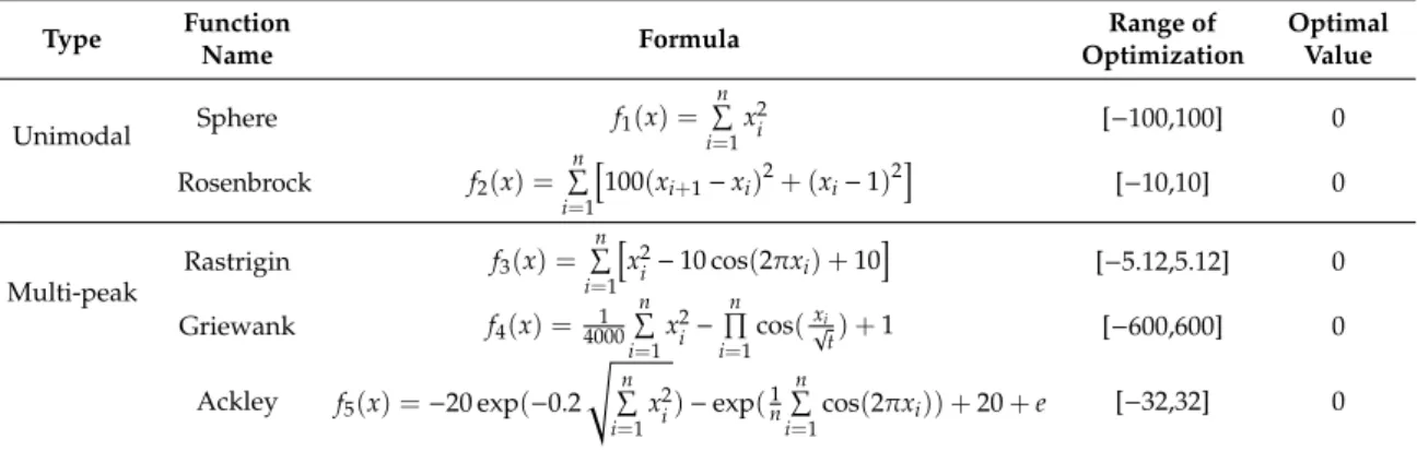
Table 1.Test Functions.
Type Function Name Formula Range of Optimization Optimal Value Unimodal Sphere f1(x) = n P i=1 x2i [−100,100] 0 Rosenbrock f2(x) = n P i=1 h 100(xi+1−xi)2+ (xi−1)2 i [−10,10] 0 Multi-peak Rastrigin f3(x) = n P i=1 h x2 i−10 cos(2πxi) +10 i [−5.12,5.12] 0 Griewank f4(x) =40001 n P i=1 x2 i− n Q i=1 cos(x√i t) +1 [−600,600] 0 Ackley f5(x) =−20 exp(−0.2 s n P i=1 x2 i)−exp( 1 n n P i=1cos (2πxi)) +20+e [−32,32] 0 4.2. Analysis of Results
This experiment was programmed using Matlab. It was run 20 times independently on a HP PC with Intel(R) Core(TM) i5-2450M CPU, 2.50 GHz RAM 4.00 GB. The algorithm parameters were set as follows: The adaptive dynamic disturbance strategy for differential evolution (ADDSDE) algorithm, population number N= 50,Fmax= 0.9, Fmin = 0.2,CRmax =0.9, CRmin = 0.2,Q= 15, δ=1×10⁻⁶, the parameter settings of the comparison algorithm DE, SADE and CAPSO are the same as the original. Consider the cases when variable dimension D=30 and D=50. The number of iterations is appropriately changed according to the complexity of each test function. The optimal value, average optimal value and standard deviation of each algorithm are shown in Tables2and3, and the convergence curve of each algorithm is shown in Figure1.
As can be seen from Tables2and3, the optimization result of the ADDSDE algorithm is significantly higher than that of the other three algorithms. For the five standard test functions selected, the ADDSDE algorithm can obtain the optimal value 0, except f5=Ackley function. The convergence accuracy is optimal. The standard deviation shows that the ADDSDE algorithm is very stable. For ill-conditioned high-dimensional complex functions, other algorithms cannot get the theoretical optimal value, some algorithms are far from the theoretical optimal value, and the stability of the algorithm is not satisfactory. From Tables2and3, it can be seen that with the increase of the dimension of the solution, the evolutionary abilities of other algorithms also decrease accordingly with different degrees.
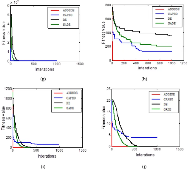
Analyzing the convergence curve of each algorithm in Figure1, we know that the convergence curve of ADDSDE converges to the optimal solution almost at the speed of vertical descent. Additionally, its optimization ability is strong, and the convergence accuracy is high. Even for high-dimensional solutions, it can be quickly fixed to the optimal position. Due to the complexity of the function and the high dimension of the problem, the other comparison algorithms are easily trapped in the local optimumand the convergence speed is also slow.
Table 2.30-dimensional function optimization results.
Function Algorithm Optimal Value Average Optimum Standard Deviation
f1 DE 8.10×10⁻⁶ 1.02×10⁻⁵ 2.84×10⁵ SADE 1.10×10⁻¹¹ 3.67×10⁻¹¹ 8.41×10⁻¹² CAPSO 5.72×10⁻¹³ 1.29×10⁻¹² 4.91×10⁻¹³ ADDSDE 0 0 0 f2 DE 2.57×101 3.59×101 7.96×100 SADE 1.83×101 2.65×101 6.33×100 CAPSO 5.42×100 7.56×100 1.41×100 ADDSDE 0 0 0 f3 DE 7.94×101 1.19×10² 2.91×101 SADE 3.01×101 3.59×101 6.21×100 CAPSO 2.10×101 2.53×101 5.31×100 ADDSDE 0 0 0 f4 DE 0 3.69×10⁻⁴ 1.65×10⁻³ SADE 0 0 0 CAPSO 8.62×10⁻¹ 9.52×10⁻¹ 6.80×10⁻² ADDSDE 0 0 0 f5 DE 1.10×10⁻⁹ 9.86×10⁻⁹ 1.37×10⁻⁸ SADE 5.48×10⁻¹¹ 6.55×10⁻¹¹ 4.39×10⁻¹¹ CAPSO 3.05×100 3.48×100 2.61×100 ADDSDE 9.56×10⁻¹⁶ 9.56×10⁻¹⁶ 0
Table 3.50-dimensional function optimization results.
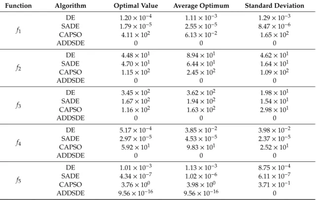
Function Algorithm Optimal Value Average Optimum Standard Deviation
f1 DE 1.20×10⁻⁴ 1.11×10⁻³ 1.29×10⁻³ SADE 1.79×10⁻⁵ 2.55×10⁻⁵ 8.47×10⁻⁶ CAPSO 4.11×10² 6.13×10⁻² 1.65×10² ADDSDE 0 0 0 f2 DE 4.48×101 8.94×101 4.62×101 SADE 4.70×101 6.44×101 1.64×101 CAPSO 1.15×10² 2.45×10² 1.09×10² ADDSDE 0 0 0 f3 DE 3.45×10² 3.62×10² 1.98×101 SADE 1.67×10² 1.94×10² 1.54×101 CAPSO 1.16×10² 1.63×10² 2.98×101 ADDSDE 0 0 0 f4 DE 5.17×10⁻⁴ 3.85×10⁻² 3.98×10⁻² SADE 2.97×10⁻⁵ 4.53×10⁻⁵ 2.37×10⁻⁵ CAPSO 5.92×101 9.83×101 2.52×101 ADDSDE 0 0 0 f5 DE 1.01×10⁻³ 1.13×10⁻³ 8.75×10⁻⁴ SADE 4.34×10⁻⁷ 1.02×10⁻⁶ 6.11×10⁻⁷ CAPSO 3.76×100 3.98×100 3.71×10⁻¹ ADDSDE 9.56×10⁻¹⁶ 9.56×10⁻¹⁶ 0
(a) (b)
(c) (d)
(e) (f)
(g) (h)
(i) (j)
Figure 1. Convergence curve of each algorithm: (a) Function f1 = Sphere when D = 30; (b) Function f2
= Rosenbrock when D = 30; (c) Function f3 = Rastrigin when D = 30; (d) Function f4 = Griewank when D = 30; (e) Function f5 = Ackley when D = 30; (f) Function f1 = Sphere when D = 50; (g) Function f2 = Rosenbrock when D = 50; (h) Function f3 = Rastrigin when D = 50; (i) Function f4 = Griewank when D = 50; and (j) Function f5 = Ackley when D = 50.
Analyzing the convergence curve of each algorithm in Figure 1, we know that the convergence curve of ADDSDE converges to the optimal solution almost at the speed of vertical descent. Additionally, its optimization ability is strong, and the convergence accuracy is high. Even for high-dimensional solutions, it can be quickly fixed to the optimal position. Due to the complexity of the function and the high dimension of the problem, the other comparison algorithms are easily trapped in the local optimumand the convergence speed is also slow.
5. Conclusions
For the solution of high-dimensional complex optimization problems, many improved DE algorithms still have many deficiencies in solution accuracy, speed, and so on. For this reason, this paper uses the advantages of the standard differential evolution (DE) mutation strategy to improve and combine mutation strategies based on chaotic mapping theory. The control parameters are adaptively weighted, and Gaussian perturbation strategies are adopted in the later iterations to prevent prematureness and jumping out of local optima, thus constituting an adaptive dynamic disturbance strategy differential evolution algorithm (ADDSDE). In order to verify the feasibility, effectiveness and optimization of the algorithm, five standard tests were selected for performance testing and compared with the DE algorithm, the SADE algorithm and the CAPSO algorithm.
Figure 1.Convergence curve of each algorithm: (a) Function f1=Sphere when D=30; (b) Function f2=Rosenbrock when D=30; (c) Function f3=Rastrigin when D=30; (d) Function f4=Griewank when D=30; (e) Function f5=Ackley when D=30; (f) Function f1=Sphere when D=50; (g) Function f2=Rosenbrock when D=50; (h) Function f3=Rastrigin when D=50; (i) Function f4=Griewank when D=50; and (j) Function f5=Ackley when D=50.
5. Conclusions
For the solution of high-dimensional complex optimization problems, many improved DE algorithms still have many deficiencies in solution accuracy, speed, and so on. For this reason, this paper uses the advantages of the standard differential evolution (DE) mutation strategy to improve and combine mutation strategies based on chaotic mapping theory. The control parameters are adaptively weighted, and Gaussian perturbation strategies are adopted in the later iterations to prevent prematureness and jumping out of local optima, thus constituting an adaptive dynamic disturbance strategy differential evolution algorithm (ADDSDE). In order to verify the feasibility, effectiveness and optimization of the algorithm, five standard tests were selected for performance testing and compared with the DE algorithm, the SADE algorithm and the CAPSO algorithm. Finally, the simulation results show that when the algorithm is applied to high-dimensional and complex optimization problems, it can still quickly converge to the theoretical optimal value. It has a strong ability of global exploration and jumping out of the local optimal. Besides, the algorithm is stable and has a certain reference value and promotion value, which provide assistance in solving high-dimensionaland complex problems in engineering and information science.
Author Contributions:T.W. designed the main idea, the chaotic mapping strategy and the adaptive adjustment strategies of the manuscript. K.W. designed the weighted dynamic mutation Strategy and disturbance mutation strategy of the manuscript. T.D. implemented the algorithm and analyzed the experimental results. X.C. revised the manuscript and perfected the language of the manuscript. All authors have read and agreed to the published version of the manuscript.
Funding:This research was fundedby the National Social Science Foundation of China (No. 15CGL001). Conflicts of Interest:The authors declare no conflict of interest.
References
1. Storn, R.; Price, K. Differential evolution a simple and efficient heuristic for global optimization over continuous spaces.J. Glob. Optim.1997,11, 341–359. [CrossRef]
2. Price, K.; Storn, R.M.; Lampinen, J.A.Differential Evolution: A Practical Approach to Global Optimization; Natural Computing Series; Springer: New York, NY, USA, 2005.
3. Bas, E. The Training Of Multiplicative Neuron Model Based Artificial Neural Networks With Differential Evolution Algorithm For Forecasting.J. Artif. Intell. Soft Comput. Res.2016,6, 5–11. [CrossRef]
4. Bao, J.; Chen, Y.; Yu, J.S. A regeneratable dynamic differential evolution algorithm for neural networks with integer weights.Front. Inf. Technol. Electron. Eng.2010,11, 939–947. [CrossRef]
5. Lakshminarasimman, L.; Subramanian, S. A modified hybrid differential evolution for short-term scheduling of hydrothermal power systems with cascaded reservoirs. Energy Convers. Manag. 2008,49, 2513–2521. [CrossRef]
6. Xu, Y.; Dong, Z.Y.; Luo, F.; Zhang, R.; Wong, K.P. Parallel-differential evolution approach for optimal event-driven load shedding against voltage collapse in power systems.IET Gener. Transm. Distrib.2013,8, 651–660. [CrossRef]
7. Berhan, E.; Krömer, P.; Kitaw, D.; Abraham, A.; Snavel, V. Solving Stochastic Vehicle Routing Problem with Real Simultaneous Pickup and Delivery Using Differential Evolution. InInnovations in Bio-inspired Computing and Applications, Proceedings of the 4th International Conference on Innovations in Bio-Inspired Computing and Applications, IBICA 2013, Ostrava, Czech Republic, 22–24 August 2013; Springer: Berlin/Heidelberg, Germany, 2014; Volume 237, pp. 187–200.
8. Teoh, B.E.; Ponnambalam, S.G.; Kanagaraj, G. Differential evolution algorithm with local search for capacitated vehicle routing problem.Int. J. Bio Inspired Comput.2015,7, 321–342. [CrossRef]
9. Pu, E.; Wang, F.; Yang, Z.; Wang, J.; Li, Z.; Huang, X. Hybrid Differential Evolution Optimization for the Vehicle Routing Problem with Time Windows and Driver-Specific Times.Wirel. Pers. Commun. 2017,95, 1–13. [CrossRef]
10. Lai, M.Y.; Cao, E.B. An improved differential evolution algorithm for vehicle routing problem with simultaneous pickups and deliveries and time windows.Eng. Appl. Artif. Intell.2010,23, 188–195. 11. Al-Turjman, F.; Deebak, B.D.; Mostarda, L. Energy Aware Resource Allocation in Multi-Hop Multimedia
Routing via the Smart Edge Device.IEEE Access2019,7, 151203–151214. [CrossRef]
12. Jazebi, S.; Hosseinian, S.H.; Vahidi, B. DSTATCOM allocation in distribution networks considering reconfiguration using differential evolution algorithm. Energy Convers. Manag. 2011, 52, 2777–2783. [CrossRef]
13. Wu, K.J.; Li, W.Q.; Wang, D.C. Bifurcation of modified HR neural model under direct current.J. Ambient Intell. Humaniz. Comput.2019. [CrossRef]
14. Kotb, Y.; Ridhawi, I.A.; Aloqaily, M.; Baker, T.; Jararweh, Y.; Tawfik, H. Cloud-Based Multi-Agent Cooperation for IoT Devices Using Workflow-Nets.J. Grid Comput.2019,17, 625–650. [CrossRef]
15. Reddy, S.S. Optimal power flow using hybrid differential evolution and harmony search algorithm.Int. J. Mach. Learn. Cybern.2018,10, 1–15. [CrossRef]
16. Sangaiah, A.K.; Medhane, D.V.; Han, T.; Hossain, M.S.; Muhammad, G. Enforcing Position-Based Confidentiality with Machine Learning Paradigm Through Mobile Edge Computing in Real-Time Industrial Informatics.IEEE Trans. Ind. Inform.2019,15, 4189–4196. [CrossRef]
17. Sangaiah, A.K.; Samuel, O.W.; Li, X.; Abdel-Basset, M.; Wang, H. Towards an efficient risk assessment in software projects–Fuzzy reinforcement paradigm.Comput. Electr. Eng.2017. [CrossRef]
18. Qiu, T.; Wang, H.; Li, K.; Ning, H.; Sangaiah, A.K.; Chen, B. SIGMM: A Novel Machine Learning Algorithm for Spammer Identification in Industrial Mobile Cloud Computing. IEEE Trans. Ind. Inform. 2019, 15, 2349–2359. [CrossRef]
19. Jamdagni, A.; Tan, Z.Y.; He, X.J.; Nanda, P.; Liu, R.P. RePIDS: A Multi Tier Real-time Payload-Based Intrusion Detection System.Comput. Netw.2013,57, 811–824. [CrossRef]
20. Autili, M.; Mostarda, L.; Navarra, A.; Tivoli, M. Synthesis of decentralized and concurrent adaptors for correctly assembling distributed component-based systems.J. Syst. Softw.2008,81, 2210–2236. [CrossRef] 21. Zhang, S.; Liu, Y.; Li, S.; Tan, Z.; Zhao, X.; Zhou, J. FIMPA: A Fixed Identity Mapping Prediction Algorithm
in Edge Computing Environment.IEEE Access2020,8, 17356–17365. [CrossRef]
22. Ambusaidi, M.A.; He, X.; Nanda, P.; Tan, Z. Building an Intrusion Detection System Using a Filter-Based Feature Selection Algorithm.IEEE Trans. Comput.2016,65, 2986–2998. [CrossRef]
23. Aljeaid, D.; Ma, X.; Langensiepen, C. Biometric identity-based cryptography for e-Government environment. In Proceedings of the Science & Information Conference, London, UK, 27–29 August 2014; IEEE: Piscataway, NJ, USA, 2014; pp. 581–588.
24. Ramirez, R.C.; Vien, Q.T.; Trestian, R.; Mostarda, L.; Shah, P. Multi-path Routing for Mission Critical Applications in Software-Defined Networks. In Proceedings of the International Conference on Industrial Networks and Intelligent Systems, Da Nang, Vietnam, 27–28 August 2018; Springer: Cham, Switzerland, 2018. 25. Brest, J.; Greiner, S.; Boskovic, B.; Mernik, M.; Zumer, V. Self-Adapting Control Parameters in Differential Evolution: A Comparative Study on Numerical Benchmark Problems.IEEE Trans. Evol. Comput.2006,10, 646–657. [CrossRef]
26. Wainwright, M.J. Structured Regularizers for High-Dimensional Problems: Statistical and Computational Issues.Annu. Rev. Stat. Its Appl.2014,1, 233–253. [CrossRef]
27. Sun, G.; Peng, J.; Zhao, R. Differential evolution with individual-dependent and dynamic parameter adjustment.Soft Comput.2017,22, 1–27. [CrossRef]
28. Chiou, J.P.; Chang, C.F.; Su, C.T. Variable scaling hybrid differential evolution for solving network reconfiguration of distribution systems.IEEE Trans. Power Syst.2005,20, 668–674. [CrossRef]
29. Wang, H.; Wu, Z.; Rahnamayan, S. Enhanced opposition-based differential evolution for solving high-dimensional continuous optimization problems.Soft Comput.2011,15, 2127–2140. [CrossRef] 30. Ali, M.Z.; Awad, N.H.; Suganthan, P.N. Multi-population differential evolution with balanced ensemble of
mutation strategies for large-scale global optimization.Appl. Soft Comput.2015,33, 304–327. [CrossRef] 31. Trivedi, A.; Srinivasan, D.; Biswas, S.; Reindl, T. A genetic algorithm—Differential evolution based hybrid
framework: Case study on unit commitment scheduling problem.Inf. Sci.2016,354, 275–300. [CrossRef] 32. Ou, C.M. Design of block ciphers by simple chaotic functions. Comput. Intell. Mag. IEEE2008,3, 54–59.
[CrossRef]
33. Shen, Y.; Wang, Y. Operating Point Optimization of Auxiliary Power Unit Using Adaptive Multi-Objective Differential Evolution Algorithm.IEEE Trans. Ind. Electron.2016,64, 115–124. [CrossRef]
34. Qin, A.K.; Huang, V.L.; Suganthan, P.N. Differential Evolution Algorithm with Strategy Adaptation for Global Numerical Optimization.IEEE Trans. Evol. Comput.2009,13, 398–417. [CrossRef]
35. Ying, W.; Zhou, J.; Lu, Y.; Qin, H.; Wang, Y. Chaotic self-adaptive particle swarm optimization algorithm for dynamic economic dispatch problem with valve-point effects.Energy Convers. Manag.2011,38, 14231–14237.
©2020 by the authors. Licensee MDPI, Basel, Switzerland. This article is an open access article distributed under the terms and conditions of the Creative Commons Attribution (CC BY) license (http://creativecommons.org/licenses/by/4.0/).