Big Data Preprocessing for Multivariate Time Series Forecast

(1)

Big Data Preprocessing for Multivariate Time

Series Forecast

UNIVERSITY OF TURKU Department of Future Technologies Master of Philosophy Thesis Computer Science June 2020 Mikael Kylänpää Supervisors: Tapio Pahikkala

The originality of this thesis has been checked in accordance with the University of Turku quality assurance system using the Turnitin OriginalityCheck service.

(2)

TURUN YLIOPISTO

Tulevaisuuden teknologioiden laitos

MIKAEL KYLÄNPÄÄ: Big datan esikäsittely usean muuttujan aikasarjojen ennustamiseen

Pro Gradu -tutkielma, 79 s. Tietojenkäsittelytieteet Kesäkuu 2020

Turun yliopiston laatujärjestelmän mukaisesti tämän julkaisun alkuperäisyys on tarkastettu Turnitin OriginalityCheck -järjestelmällä.

Big data -alustat helpottavat isojen datamäärien talletusta ja hallintaa. Niiden haittapuolena on kuitenkin laaja data-analyysiin vaadittava esikäsittelyn tarve, mikäli halutaan käyttää tavanomaisia analyysimenetelmiä. Erityisen haastavaksi todetaan aikasarjojen muuntaminen alustan tarjoamasta muodosta ohjatun koneoppimisen vaatimaan taulumuotoon, koostuen ennustettavasta kohdemuuttujasta sekä muista ominaisuusmuuttujista. Tässä tutkielmassa tutkitaan usean muuttujan aikasarjadatan esikäsittelyä, sekä käsitellyn datan ennustamista koneoppimismenetelmillä, kuten neuroverkoilla ja tukivektorimallinnuksella. Tutkimusmenetelmät perustuvat kirjallisuuteen datan esikäsittelystä ja aikasarja-analyysistä, mutta myös uusia menetelmiä kehitetään, kuten lokitasoon perustuva kohdemuuttuja sekä muuttujien arvojakaumaan perustuva karsiminen. Ennustustulokset jättävät kuitenkin toivomisen varaa, mikä kertoo big datan mallinnuksen vaikeudesta. Epäiltyinä syinä ovat liian vähäinen malliparametrien ja esikäsittelyvalintojen optimointi, joiden täydentäminen vaatisi resursseihin nähden liian kattavaa testausta.

Avainsanat: big data -alustat, datan esikäsittely, aikasarja-analyysi, ohjattu koneoppiminen

(3)

UNIVERSITY OF TURKU

Department of Future Technologies

MIKAEL KYLÄNPÄÄ: Big Data Preprocessing for Multivariate Time Series Forecast

Master of Philosophy Thesis, 79 p. Computer Science

June 2020

The originality of this thesis has been checked in accordance with the University of Turku quality assurance system using the Turnitin OriginalityCheck service.

Big data platforms alleviate collecting and organizing large datasets of varying content. A downside of this is the heavy preprocessing required to analyze their data by conventional analysis techniques. Especially time series data is found challenging to transform from platform-provided raw format into tables of feature and target values, required by supervised machine learning models. This thesis presents an experiment of preprocessing a data-platform-extracted collection of multivariate time series and forecasting it by machine learning models such as neural networks and support vector machines. Reviewed techniques of data preprocessing and time series analysis literature are utilized, but also custom solutions such as log level-based target variable, and value-distribution-based feature elimination are developed. No significant forecasting accuracies are achieved, which indicates the difficulty of modelling big data. The expected reason for this is the inadequate validation of model parameters and preprocessing decisions, which would require excessive testing to improve.

Keywords: Big data platforms, data preprocessing, time series analysis, supervised machine learning

(4)

Abbreviations and Acronyms

AC Autocorrelation

ANN Artificial neural network

AR Autoregression

ARIMA Autoregressive integrated moving average ARMA Autoregressive moving average

AUC Area under curve B2B Business-to-business

BP Backpropagation

FE Feature extraction FPR False positivity rate FS Feature selection GRU Gated recurrent unit IR Instance reduction IS Instance selection

JMX Java management extension kNN K-nearest-neighbors

LSTM Long short-term memory

MA Moving average

ML Machine learning

MLP Multi-layer perceptron MSE Mean squared error NoSQL Not only SQL OHE One-hot-encoding PAC Partial autocorrelation RNN Recurrent neural network RVM Relevance vector machine SRs Secure relays

SVM Support vector machine SVR Support vector regression TPR True positivity rate VAR Vector autoregression

(7)

1 Introduction

Many of today’s digital services are built around data. Varying data is collected from not just the main processes but from all around the services for later uses, including knowledge discovery by data analysis and machine learning (ML). Traditional data storage techniques such as relational databases have proven incompatible with the volume and dynamics of these large scale, distributed, and simultaneously increasing data collections, often referred to as big data. This has led to use of stand-alone data platform software such as Hadoop [1] and Elasticsearch [2], that are especially designed to operate such collections. One of the reasons enabling their advantage is the relieved restriction on data format. This is also known as schema-less approach, where all sorts of data can be collected without preorganization of table structures. A common storage format is a JSON-based document store, where the documents can contain highly altering contents, yet capable of fast and programming-oriented querying without requiring external database transformations.

Consequently, there is a certain disadvantage in analyzability of the less-structures data collections. Most data analysis and ML methods operate with table-like data, consisting of columns and rows. Therefore, applying ML on big data requires additional transformation from raw data into analyzable table-format. In contrast, traditional databases are table-oriented by nature and hence much easier to prepare for analysis. Another key issue of big data analysis is the size of the collections. Many ML-methods are computationally demanding already on small datasets, so applying them on big data insists means of transforming the data into smaller scale. To overcome such issues, this study presents a review on various data preprocessing methods, along with a practical experiment of preparing a dataset of such scope for ML analysis.

A special factor is that the experimented dataset contains no predefined target variables to predict by ML. Instead, selecting or crafting this variable is considered a part of the preprocessing. In that regard, this study represents a nowadays common data analysis task, where a client provides data and invests in exploratory data analysis, hoping for

(8)

potential findings unknown in beforehand. In this specific case the provided dataset is a time series, and the goal is to preprocess it by selecting as informative as possible feature

or input variables and the target or output variable to forecast. As the learning task, this study focuses on multivariate time series analysis and forecast, where multivariate refers to analyzing multiple concurrent time series, and their effects on each other.

Time series analysis has traditionally referred to statistical techniques by Box and Jenkins [3], but an increasing amount of ML alternatives have been published, due to recent advance in the field. ML has unique characteristics as opposed to traditional methods. One of them is the preliminary parameter learning process i.e. model training for which there are two categories or learning setups. In supervised learning setup the dataset is labeled, making each instance consist of feature values along with a class label or a numerical target value. The former label type is known as classification and the latter as

regression. Unsupervised learning, on the other hand, operates with unlabeled data, and these algorithms are used for structuring data, for instance by clustering. Time series forecast is considered supervised, as its task is to predict the target variable i.e. future, based on feature variables i.e. history of the series. Another specialty of ML is that it is usually completely data driven. For example, rather than explicitly computing the trends and cycles in a time series, as part of the method, ML-models can learn them implicitly from training data.

Amongst ML techniques, especially deep learning has proven advantageous in modelling large datasets or big data. A specific type of deep learning is recurrent neural networks (RNNs), especially designed for learning to predict sequences such as time series. RNN techniques like long short-term memory (LSTM) [4] and gated recurrent units (GRUs) [5] have shown success with non-real-time sequences like text and speech recognition, making them promising candidates also for real-time sequences focused on this study. However, a certain difference between real-time and non-real-time sequences is that the latter is much easier to scale up. For instance, a text dataset can be increased by inserting more sentences, whereas with real-time sequences the only means of increasing is to count in a longer history or more concurrent features, if such are collected. It is hence uncertain if a time series dataset will reach the level where deep learning can outperform other methods. In addition to preprocessing techniques, this study reviews also the most

(9)

common time series analysis methods, from traditional to deep learning, aiming to provide which of these are best suitable for learning real-time multivariate sequences.

(10)

2 Motivation

This thesis is done in collaboration with a Finnish IT company, henceforth referred as

company A. One of A’s services is maintaining support services for clients’ software and

business-to-business (B2B) integrations. The services operate on clients’ log and metric

data, providing real time monitoring, alerting of errors, and minimization of downtime on production environments. As its data platform, A utilizes Elasticsearch, that is distributed JSON-based querying specialized document database. For monitoring, A uses Kibana [6] and Grafana [7] that are also provided by Elasticsearch. One of the disadvantages of this system is the lack of root cause analysis capabilities, due to which the discovering of the causes must be done manually after the occurrence of the errors. As the service lacks knowledge of root causes, it is also incapable of predicting an upcoming error when a root cause appears. This study aims to provide the missing predictability by developing forecasting model for a dataset extracted from A’s platform.

If successful, the model could be used as early warning system, forecasting the state of the operation for time ahead. If the predicted state were erroneous, an early warning could be triggered, enabling prohibitive processes to prevent the errors.

In order forecast on large scale data, a heavy amount of preprocessing is required. It is acknowledged that Kibana, for instance, contains a built-in ML library that requires no excessive preprocessing. However, this study focuses on which processes are required if not using platform provided functionality. This allows the use of state-of-the-art techniques that platforms such as Kibana do not necessarily utilize. As mentioned, a key step in this project is also determining the target variable which is the variable to forecast. Since the goal is to predict the state of A’s client operation, this variable should reflect

the health of the operation as well as possible. As the product of the preprocessing, three feature variable subsets are prepared along with a target variable to predict. Each subset is forecasted, and their performance is evaluated by the accuracy of the forecasts.

As the forecasting technique, also three candidate methods are experimented. Their performances are compared, to see which method performs best on given data. Additional parameters of forecast are lag distance, i.e. how much history to calculate for a prediction,

(11)

the optimal lag distance should be within one hour, and horizon from 15 to 30 minutes. The lag distance affects especially the computational complexity, as counting in more instances naturally requires more computation. A longer distance, however, could increase the accuracy of the forecast. The horizon, on the other hand, defines how far ahead to predict. It hence determines how much time there would be for prohibitive actions after a warning is triggered. A longer horizon is not necessarily a benefit, as the farther the horizon, the less accurately a model likely predicts. Thus, two horizon lengths, 15 and 30 minutes are experimented. This makes the final experimental setup of this study a cross-validation of a) 2x datasets, b) 3x preprocessed subsets, c) 3x forecasting methods, and d) 2x parameter combinations. Finally, the best performing models are evaluated also as warning systems, assessing not just their overall forecast capability, but also accuracy on triggering warnings correctly.

Study objectives summarized:

 Discover preprocessing techniques for transforming multivariate big data time series into analyzable format.

 Discover means for selecting/crafting a forecast target variable for the dataset provided.

 Discover methods for forecasting time series data of such scale.  Apply forecast and analyze the success of the set objectives.

Disregarding the objectives set above, an overall goal of this thesis is to discover universally compatible preprocessing techniques that are applicable to not just the case data, but any large-scale time series type of data. The experiments are exploratory acknowledging the null hypothesis, which is that no efficient preprocessing can be applied, and no reliable forecasts can be made on them.

The chapters are divided into two parts. Part I contains the theory of big data preprocessing, and its practical application on a client dataset provided by company A. Part II contains time series theory, along with forecast experiments on the client data that was prepared in part I.

(12)

Part I

(13)

3 Background

3.1 Big data platforms

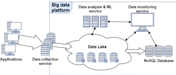
Many applications used for collecting, storing, and analyzing data can be considered as big data platforms. [8] describe the key features of them by size, complexity, and certain associated technologies such as not only SQL (NoSQL) databases e.g. Cassandra [9], MongoDB [10] and file distribution frameworks e.g. Hadoop, Elasticsearch. A key difference compared to traditional data storage is that these techniques usually require no strict schema or structure for content they store. This allows any available data source to be collected without restriction or prior organization. Big data platforms typically consist of a data lake, containing the data in raw format and a database or equivalent application, that provides indexing, organization, and better user access to this raw content. Most applications are horizontally scalable, i.e. their data can be distributed on multiple server nodes to increase storage size. Scaling horizontally allows practically infinite increase of volume. In addition, it usually provides content replication, meaning that the data is stored physically in multiple locations, which allows high availability and reliability, even if single nodes fail.

(14)

One of the most common NoSQL database types is document database. Instead of standing for the storage format, the documents function as wrapper of content, providing a uniform format for handling any contents. For example, MongoDB and Elasticsearch use JSON as the document format. As compared to traditional data storage, e.g. relational databases, JSON is faster to search, more flexible towards varying or dynamic content and supports constructs familiar to most programming languages, such as lists [11]. Another benefit of JSON is that the documents can naturally contain nested elements i.e. parents and children, whereas a relational database would require separate tables and foreign keys for handling such recursion. Lastly, querying JSON is fast, as most programming languages have ready-made implementations for operating with the format. An additional feature of some data platforms is being real time. This means that collection of data, from source to storage is continuous. Examples of real time data sources are

application log files and sensor readings that a collecting service “listens to” and transmits

into the platform simultaneously. This type of collection allows utilizing the data for real time alerting and monitoring purposes. Associating instances with timestamps also turns data into time series, enabling time series analysis. Many big data platforms provide a complete software, consisting of a storage unit or framework e.g. Hadoop, Elasticsearch, a UI client for control and monitoring e.g. Splunk [12], Kibana, and a separate component for collecting real time data e.g. Sqoop [13], Logstash [14]. Additional modules are often provided as plugins, for example for advanced visualization e.g. Grafana and ML purposes e.g. Mahout [15].

3.2 Issues with data analysis & ML

The schema-less approach has a lot of advantages concerning data collection and storage. However, as a downside, it may hinder data analysis capabilities. This chapter presents such issues, affecting especially ML-modelling on real time and big data platforms. Five main issues, namely size, dimensionality, format, missing values, and data outages are focused. In practice, the issues are solved by various steps of data preprocessing, which is a fundamental part of any data analysis study and challenging for big data.

(15)

3.2.1 Size

The foremost issue with large datasets is their size. Although general computational power has increased due to distributed and parallel computation techniques like GPU-processing, a combination of large data with complex models might still be a restriction to many studies. In turn, cloud computing providers offer high-performance computing e.g. Google Colab, as a service, but this study focuses on capabilities without using such services. If unable to utilize high-performance computing, a practical approach to deal with size issues is to reduce the volume in preprocessing.

The processes of reducing data by instances are known as instance reduction and selection [16]. Instance reduction (IR) means selecting instances to drop out, whereas instance selection (IS) means selecting the instances to keep in data. The problem of IR/IS is the loss of information value that it might cause. For example, if a dataset consists of many instances of class A but only few instances of B, a bad IR could drop all instances of B, hence completely corrupting the information. This problem affects especially unlabeled datasets, where stratification, i.e. ensuring correct distribution of labels cannot be applied. A basic application of IR for example for survey-datasets, is to remove noisy and redundant instances. This process is also known as data cleaning.

List of common IS/IR methods [16,17]:

 Random sampling – Drops instances randomly. The only goal is to reduce volume.  Stratified sampling – Drops instances randomly amongst classes, maintaining

original class distribution.

 Outlier detection – Reducing the data size by dropping statistical outliers. This is applicable only on numerical features, and with datasets where outliers exist.

 RT1, RT2, RT3 – Advanced reduction techniques by [18]. These methods calculate the effect of instances for the learning task, dropping out redundant ones. The performances on multiple learning tasks were reportedly increased, utilizing them.

(16)

3.2.2 Dimensionality

Another issue related to data size is dimensionality, which means the number of features for an instance. In addition to increasing computation time, dimensionality also causes issues known as curse of dimensionality [19]. A practical example of this is if a dataset has few instances but many features, each instance is likely to appear distant of each other, if all features are concerned. This makes it difficult to find similarity between any instances of data. Because of this, high dimensionality also requires high number of instances for similarities to appear. High dimensionality also restricts the model selection available for an analysis task. For example, distance-based methods’ such as support

vector machine’s (SVM) and k-nearest-neighbors (kNN) classification’s computational

complexity is directly proportional to number of features in data, making them easily too inefficient for highly dimensional datasets. High dimensionality can be dealt with dimensionality reduction techniques, the most common of which being feature selection and feature extraction [16].

Feature selection (FS) refers to similar selection or drop-out than IR/IS, but amongst the feature space. The foremost part of FS is to remove features which certainly have no effect in the analysis. For example, if only persons of specific age are analyzed in a study, the feature representing age is then redundant and can be removed, as it would always contain the same value. Another example are metadata fields such as object identifiers or dates of last update, common in data platform datasets. If counted in, the redundant fields may reveal spurious correlations, i.e. coincidental correlations without actual causality. FS is also used to remove non-redundant but highly correlated features. For example, if a dataset contains individual fields for age and birthdate, the two would be 100% positively correlated, making it unnecessary to utilize both fields. Even lower levels of correlation could indicate that two features represent the same event, hence only requiring one feature for recognizing it.

[20] divide FS-techniques into filter, wrapper, and embedded methods, based on the

technique’s relation to the actual model. Filter methods analyze the data independently,

generating the final feature subset for models. Wrapper methods function together with the model, providing candidate subsets for the model, that are then evaluated to discover

(17)

the best performing one. This approach is also known as FS-cross-validation. Lastly, embedded methods refer to learning models, that have a built-in FS process. Below are presented lists of common FS methods by category.

Filter methods [16,17,21]:

 Manual – Selecting best features based on expert knowledge.

 Correlation coefficient – Selecting features that correlate most with output value or classes. Functions with numerical values.

 Chi-Squared selector – Chi-Squared test ranks categorical features’ correlation to

output value. This is like correlation coefficient but for categorical features.

 Fast Correlation-Based Filter (FCBF) – Advanced, computationally light, correlation-based filter method for highly dimensional data by [21].

Wrapper methods [20]:

 Sequential forward selection or backwards elimination – Systematically goes through each feature, evaluating its effect on performance. Selects features increasingly if they improve performance or eliminates features decreasingly if discarding them improves performance.

 Genetic algorithm – Advanced, natural selection inspired FS method. The method starts by creating random subsets and evaluating them. The best subset is then used to create a pool of new candidate subsets, and the process is repeated for the new candidates. This evolution converges to best possible subset.

Embedded methods [20,22]:

 Decision trees & Random forests – Decision tree modelling and its expansion, Random Forests are user friendly and intuitive models for example for classification

tasks. Additionally, they provide a straightforward measure of a feature’s importance

on decisions, which acts as embedded FS.

 Least absolute shrinkage and selection operator (Lasso) – A regression analysis method that applies feature selection. It can also be used to enhance other regression methods such as Ridge regression.

(18)

The other approach of dimensionality reduction is feature extraction (FE), which means creating artificial features based on original ones. This enables the use of high-dimensionality-incompatible analysis methods despite the original data contains too many features. Another benefit of reducing dimensionality is that it can be used to project data into two or three dimensions that are visually observable. This could reveal patterns such as clusters, already as such. A common subcategory of FE are space transformation methods. These create projections of high dimensional data to greatly lower dimensions. In contrast to regular FE, space transformations make the projections based on all original features, preventing information loss. One could still have the output of a model as original feature but use extracted features as input for learning tasks. A downside of FE is that it makes the analysis closer to black box, as one cannot so easily determine a single

original feature’s effect, since it is not used as such. List of common FE methods [16]:

 Matrix factorization – Matrix factorization methods like Single Value Decomposition (SVD) are used in recommender systems. However, they can also be used as feature selection algorithms. For example [23] represent a matrix factorization-based unsupervised feature extraction algorithm.

 Principal Component Analysis (PCA) – Perhaps the most common space transformation method. It projects the data to the desired number of dimensions that maximize the variance in the data.

 Independent Component Analysis (ICA) – A space transformation method like PCA but maximizes independence instead of variance. It is typically used in signal processing for separating independent sources of data.

3.2.3 Format

The schema-less approach improves the flexibility and scalability of big data platforms. However, there are multiple issues affecting the analyzability of such data. First, most data analysis methods operate with columns and rows. Each instance must populate every

(19)

column with a value, or leave it empty, i.e. populate it with null. JSON for example, requires an additional preprocessing step of converting the documents into tables. Moreover, a dynamically altering JSON or equivalent dataset, might yield a large portion of empty values, requiring more strategies for handling the nulls. Second, as JSON or equivalent might contain nested objects, they must be flattened to fit it into a table. This means unfolding all nested objects into single level, which could make the representation more complex. The unfolding process is illustrated in below, where the braces refer to parent-child relations:

input: output:

A A

B{C, E}  B.C, B.E

F{G, H{I}} F.G, F.H.I

Like format of data, also the type of features affects analysis, especially with big data. Since ML algorithms are math-based, textual features must be transformed into numerical format before analysis. Feature indexers and encoders are techniques that can be used for such transformation [24]. A discrete amount of categorical textual field values, for example species names in a dataset of plants, are straightforward to index into numbers where each number represents one species. However, more complex textual features such as actual text entries are harder to index or encode. Text mining presents techniques aiming to categorize texts to index them into numerical scale [16].

List of common indexer and encoder methods [16]:

 String indexing – Transforms a discrete set of textual labels into indexed numbers. The order of which can be defined for example by the total number of labels; the most frequent class or label being either first or last.

 One-Hot-Encoding (OHE) – A common strategy, also used for representing output classes with neural networks. In a discrete set of labels, each label is given a binary feature, yielding value 1 if an instance represents the label and 0 otherwise.

(20)

The transformation to numerical features is fundamental to any size of dataset that ML is applied to. However, especially large scale and highly dimensional data is problematic. For instance, if a dataset is already highly dimensional, OHE increases the dimensionality even further, which could introduce dimensionality issues. This has been studied [24] and [25] who propose alternative techniques as well. [24] demonstrate issues with non-standardized categorical variables. An example of such is a person’s title-field which could contain multiple entries like PhD and Ph.D, despite all referring to the very same entity. With basic OHE, these would yield two or more non-lapping features, which could corrupt the analysis as the model would interpret them as different entities. They propose

their own method, especially targeted to “dirty data” i.e. datasets with spelling mistakes

that make same entities represented by multiple accidental values. [25], on the other hand, present a comprehensive comparison of OHE against binary encoding and feature hashing, more detail of which is given below.

List of OHE alternatives [16,24,25]:

 Term frequency search – This approach is eligible for continuous textual fields. A specific term is defined as keyword, and the frequency or amount of it is scored as the new feature value.

 Stemming – This approach is like term frequency search, but instead of searching a term within texts, searches roots of terms within terms. An example is root standard

in term set standards, standardize and standardized. There are many extensions to basic stemming, such as [24]’s similarity encoding, which provide more advanced indexing or scoring of roots.

 Binary encoding – Where OHE represents features as one-bit binary, binary encoding represents them as multi-bit. For example, where OHE encodes a feature of 4 classes into 4 binary features (0,0,0,1), (0,0,1,0), (0,1,0,0), (1,0,0,0) binary encoding requires only two; (0,0), (0,1), (1,0), (1,1). This approach yields much less dimensions when encoding discrete categorical variables.

(21)

 Feature hashing – In this approach, feature values of any type are sent through a hash function, which denotes an output integer within a set of desired length. The acquired integers act as the new encoded features. Interestingly, hash collision, i.e. two separate values being hashed to same output does not drastically decrease prediction performance as heavily as expected, according to [25]’s study.

 Clustering – An ML-oriented alternative to apply feature encoding or any dimensionality reduction is to perform unsupervised learning such as clustering on desired set of features. The formed clusters can then be interpreted as feature labels.

For an even more advanced encoding strategy, [26] represent a neural network approach, resembling an autoencoder. Autoencoders are neural networks that learn complex functions for altering data representation and are therefore used for example for encoding and decoding purposes. [26]’s network functions like an autoencoder but also reducing the output dimensionality to a smaller scale. It essentially falls into the category of space transformations, but it can be also used to convert non-desired feature types such as categorical textual fields into numerical representation, which allows better modelling capability.

Feature types especially affect time series analysis. For example, statistical regression methods like ARMA-models (see 5.2) operate only on ordinal numerical values. Ordinality means that the feature can be measured as high or low compared to other instances. Many categorical features are nominal or not ordinal, meaning that their values cannot be compared to each other. An example of such is species name that represent category rather than measure. There are exceptions of ordinal categorical features such as log level. It is a textual feature commonly associated with log messages, denoting the severity of the event with values like debug, warning, or error. Since the categories measure the severity, they can be indexed into increasing order, i.e. debug: 1, warning: 2

(22)

3.2.4 Missing values

Another category especially related to the schema-less storage are missing values. Efficiently handling missing values is critical, as bad handling strategies could bias the analysis [16]. One of the primitive handling techniques is to drop out instances that have missing features. However, this is only applicable if the portion of instances with missingness is small. If not completely dropping instances, the other approach is to fill their empty fields with artificial values. This method is also known as imputation. There are various imputation strategies, i.e. criteria for what to fill the empty values with.

List of imputation strategies [17]:

 Mean or median – The most common and basic imputation strategy is to fill empty

values with feature’s or table column’s mean or median value. This is easily

extendable, for example to instead using a mean or median within a class or category.  Hot deck imputation – Find an instance that most resembles the instance with

missing value. Use this instance’s value to impute the missing one.

 Regression or classification – An advanced imputation strategy is to build a complete separate classification or regression model, that takes as input the other feature values and predicts the missing value based on statistics or model parameters if ML.

Like format, also missing values cause difficulties especially withs time series datasets for multiple reasons. First, one cannot completely drop out only instances with missing values because time series must always have fixed time intervals between instances. Second, one cannot impute empty values with 0, -1 or other fixed values, because they could be in the natural scale of some variable, for instance, temperature in Celsius. Third, one cannot impute empty values with averages or most common values, at least in a non-stationary time series (see 5.1). This is because the series could be on a peak of a trend

during the missing value’s occasion. Inserting a much smaller average value between two

(23)

More complex imputation strategies for time series have been reviewed by [27,28]. [27] studied the impact of missing values in political data analysis. The key issue affecting time series imputation in this field is the type of the missingness, e.g. informative or non-informative missingness. In the former case, a problem is that there is likely a reason why a feature value is missing, which should be concerned in the imputation. The process should also concern other features, which have values for the moment. For instance, if every other feature dive at a specific moment, the imputed value should likely dive as well. A similar problem is presented by [28], who studied missing values in multivariate scientific time series forecast with RNNs. They found missing values correlated to prediction performances also in sensorial data, e.g. health care, biological and geoscientific datasets. However, instead of applying imputation, they propose a completely new kind of GRU neural network (see 5.3.3), namely GRU-D, that functions with the empty values, rather than guessing the real value of them. This approach showed promising results; where regular RNN with imputation performed at the same level with SVM, GRU-D was able to deliver the increased performance that deep learning generally provides. The network seemingly learns to interpret null as a special class to detect patterns of. However, this likely requires a substantial portion of missing values, to learn their pattern. Relatedly, for example [29]’s RNN-experiment concerned a small amount of empty values, so imputation could be considered a minor factor regarding prediction performance.

Missing values are especially problematic in multivariate time series analysis. As described, the format and size of big data might cause missing values as such. An additional factor is the density or framerate of time series. To analyze multiple time

series’ effect on each other, they must be synchronized by framerate. This means that

each individual series must share timestamps. Hence, and additional preprocessing step is required for synchronizing the time series, which could be a heavy process especially with large datasets. A time series can be synchronized either by sparsening or densening it. Sparsening means discarding for example every nth_{instance from a series. It could lose}

information value, as the discarded instances could include informatically valuable ones. Densening, in contrast, means adding artificial instances between original ones. It does not lose information value, but could corrupt the data, if the artificial instances are

(24)

inaccurate. A synchronization process could include applying both, to obtain a uniform framerate for every time series in a dataset.

3.2.5 Data outages

A special type of missingness are data outages. Affecting especially real time data platforms, outages refer to continuous missingness of a data source or feature for a limited period. An example outage is if a sensor or collecting service malfunctions, which causes missing values or no data until it is fixed. Outages do not only refer errors, as they could also be due to regular restart or reboot of a service. Because of this, outages are especially difficult to model, as there could be multiple origins for one, either normal or erroneous. There are very few publications on how to handle outages in multivariate time series analysis. A primitive approach like with regular missing values would be to discard periods or complete features with outages occurring. However, this would lose potential information value that defines the missingness. Because an outage could cause or be caused by an event in another series or features, identifying such correlations could be critical for example in root cause analysis of an error.

If wished to benefit from outages in analysis, the biggest concern is how to represent them in the data. As described, most models cannot function with nulls, so this requires a process of labeling the outages. The difficulty of labeling depends on feature types. For example, one can simply add a new category or label representing outages for a categorical feature. However, or an ordinal and numerical feature, it is difficult to allocate a value for representing one. Intuitively, one could label outages as zeros, but with assumption that it is not in the natural scale of the feature. If so, an alternative strategy could lie in discretization. Discretization means transforming a continuous value into discrete set of ordinal categories. An example discretization is transforming temperature degrees into classes like freeze, around-zero, and heat. This set of classes could then be expanded with a new class that represents outage. However, it would still not satisfy the ordinality requirement for most features, as an outage cannot be measured as high or low, for example by temperature. Especially statistical time series methods (see 5.2) require ordinality, also making discretization ineligible.

(25)

Among the few publications concerning the issue is [30]’s study of missing event

prediction in sensor data streams. For an outage situation, they utilized Kalman filters, that is a recursive data approximation function for predicting the missing sensor readings. However, this approach merely predicts the missing values, rather than utilizing the informative missingness in the outages. A candidate method that could benefit from outage information is the GRU-D neural network proposed by [28], as it particularly analyzes patterns of missingness.

(26)

4 Case study – Preprocessing for time series

analysis

4.1 Target & objectives

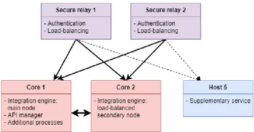
The case study is targeted on a specific client of company A, henceforth client B. B’s

production operation runs on five host machines that contain software components such as integration engine and API manager. Their main process are B’s B2B-integrations that conduct the internal and outbound message traffic, including orders and other logistical

messages between various physical and virtual endpoints. The integration engine’s load

is balanced into two hosts, namely cores 1 and 2. The other three hosts in the cluster perform additional supportive operations such as secure relaying. In this chapter, client B’s operational data is preprocessed and prepared for time series analysis in part II of the study. Both custom-made techniques, and methods reviewed in chapter 3 are experimented, to create a computationally compact and informative dataset from the raw data.

(27)

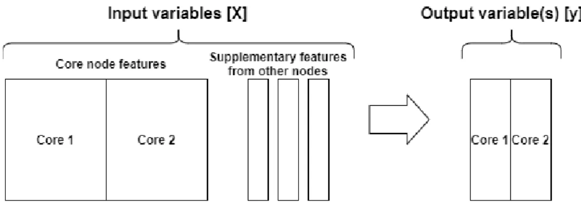
As for any data prediction task, the first consideration is which variables to analyze and which to predict. Since cores 1 and 2 host the main operation, these two also produce the most impactful logs and metrics to analyze. Considering this, the preprocessed dataset should contain mostly core features, so the models do not overfit on the supplementary behavior. The target or output variable should also represent the cores. Although being supplementary of the main operation, the other three nodes could provide additional root causes that affect the behavior of the cores, and hence should not be considered as input features. The preprocessing objectives are illustrated in fig. 3:

Figure 3 The forecasting methods analyze input variables to predict output variables. The boxes indicate which host the features or variables are selected from. The output variable should present the predicted state of errors in both cores.

As for the target variable, since not being predefined, one must either select a representative feature from the original features as such or extract it from the original features. Most forecasting methods cannot predict multiple targets, so if selecting multiple targets, the forecast would need to be repeated for each individual log level (see 3.2.3). Hence, the goal is to craft a single target to predict. Since company A’s role in

client B’s operation is to ensure system health, the target variable should reflect the health of the operation. There are two key variables in the data, that are expected to reflect the health best; the log level features that the data contains plenty of, and outages that occur from time to time in all features. Log levels are straightforward indicators of errors as

(28)

such, whereas outages could be caused by a critical error in the system making them potentially informative targets to forecast (see 3.2.5).

4.2 Dataset

The dataset of client B is a collection of data tables provided as csv-files. These tables were created in a separate data engineering project [31], acquiring the data from Elasticsearch, transforming it from JSON into tables, and reducing the volume by a large scale. The final tables contain multivariate time series, from the five host machines in B’s

production environment. There are from two to three tables per each host, each table containing a specific source of data in it. The source types are described below:

1. Filebeat – Contains application log data. This includes log levels and additional status information of logs. The message contents are filtered out due to their excessive lengths and complexity to analyze. Filebeat-sources have a dynamic collection interval, as they are collected simultaneously when produced by services. The features of the source are mostly categorical variables.

2. Metricbeat – Contains system metrics such as CPU and memory usage of hosts. The readings are collected at fixed rates within configured intervals. All metricbeat -features are categorical.

3. Jmx-beat – Contains Java management extension (JMX) statistics, i.e. metrics from important java processes. These readings are also numerical and collected within configured intervals.

The table rows are ordered so that the first row of each table represents the first lag and last row the last lag in the time series. The raw data contains from 4 to 63 features per each table. The collection intervals above refer to the rate that the data is collected to A’s

Elasticsearch cluster. The tables are synchronized to uniform framerates, so that the nth

(29)

originally 8 months: April 18th _–_{November 15}th_{. However, the provided data is divided}

into two subsets. Dataset 1 contains the full period with a 5-minute framerate (60780 rows), and dataset 2 only the last 2 months but with a 1-minute framerate (87900 rows). The advantage of dataset 1 is that it covers the full period, including a wider history. However, the original data is generated denser than 5 minutes, so the synchronization process has decreased event accuracy. In contrast, dataset 2 is closer to the original density but covers a shorter history. In 4.4.2, the length of dataset 2 is further shortened to 50500 rows for reasons explained.

As a remark, both datasets contain a lot of missing values, for two reasons. First, the data is highly dimensional, and the collection rates vary between individual features and tables. Because of this, some of the features have been densened by inserting empty values between the original values to match the uniform framerates. Second, there are a lot of outages, that appear as missing values.

4.3 Missing values & outages

The foremost problem of this study to solve are missing values. This is because most forecasting methods and preprocessing techniques cannot operate with nulls and cannot be used before replacing these. A key factor affecting the replacement are outages. There are two types of them: normal outages due to service reboots or updates, and outages caused by errors. Moreover, outages can take place for a single service, or for the whole system.

A certain property of outages in is that they act differently on logs and metrics. Since logs are written based on actions of the process, a missing log could represent a healthy period, where in contrast, dense logging could indicate errors. Hence, missing values are considered natural for filebeat-tables. Metrics, on the other hand, are collected at fixed rates. Therefore, missing metrics can indicate either a sparser collection interval or an outage. Because of this, missingness should be treated differently on metricbeat and jmx-beat tables. Also, as shown by [28], there could be information value in patterns of missingness, so the missing values should be kept as such rather than imputing. The next

(30)

proposed methods aim to classify outages either as a) natural missing value due to sparser collection rate, b) normal outage due to service restart, orc) error-caused outage due to system malfunction. The natural missing values could then be imputed, and the outages labelled either as normal or erroneous outages.

4.3.1 Outage detection

To address the described requirements, the first process is trying to separate natural missing values from outages. The following proposed method analyzes complete missing rows for separating the instances. As filebeat-outages are treated differently, this method is applied only on metricbeat and jmx-beat tables. The basic idea of it is to check whether some values of a row are missing, or all of them, as all features missing would refer to a metric-wide outage. The method is presented as algorithm below:

iterate table by rows:

if some, but not all features of row are 'null': impute missing values

else if all features of row are 'null': label row as outage

By experimenting, it is noted that with client B’s data, this method still yields a heavy

portion of outages in metricbeat. Below is an illustration of the resulting outage labels on

(31)

Figure 4 Dataset 1 (left), dataset 2 (right). Metricbeat outages (blue), jmx-beat outages (orange). The x-axis represents the full analysis periods on both datasets 1 and 2.

The problem of heavy missingness is that as the metrics are numerical, they would also need to be imputed with a numerical value, rather than a new category representing them (see 3.2.4). However, the regularity of the missingness in metricbeat suggests that they are caused by the sparser collection, rather than actual outages occurring. Unlike

metricbeat, jmx-beat’s original collection intervals are denser than the synchronized interval, so there are no sparseness-caused missingness. Because of this, the outages present in jmx-beat (orange) are likely indicating actual system-wide outages. More evidence is given by the fact that, there are also missing values in metricbeat and filebeat, during jmx-beat’s outages. Since jmx-beat-tables represent outages so well, the approach is changed to labeling only the outages detected by jmx-beat. Hence, the outages detected in metricbeat only are handled like regular missing values, which is performed in 4.3.4.

4.3.2 Missing value imputation

After the outages have been detected, the imputation strategy for other missing values must be selected. The imputation is applied to the missing values that are not considered as outages in 4.3.1. A key factor considering the strategy is the nature of data. An expected property of server metric data such as client B’s is that the metrics should keep previous

state if no explicit changes occur. There should also be no dirty data features (see 3.2.3), as all features are recorded by sensor rather than human. Lastly, since working with time

(32)

3.2.4). Acknowledging these, it is decided to impute missing values based on the preceding active value for each feature. If the missing value follows an outage, the next active value should be used instead, because the value is more likely to represent the state after the outage, rather than state before it. The process is also represented by following algorithm:

1. iterate table by rows (top-down): iterate row by values:

if row is not outage and value is 'null':

impute with corresponding value from preceding row 2. repeat step 1. bottom-up

Iteration 1. imputes missing values with the last collected value of the feature if one exists within an outage-less period. This leaves all missing values that follow an outage empty. Iteration 2. repeats the process but from bottom to top, so the missing values after outages get imputed with the next collected value of the feature.

4.3.3 Outage-error correlation

After detecting outages, a consideration is whether it is possible to segregate them as normal e.g. updates and reboots, or error-caused. The distinction between the two could benefit the forecast, as one is only interested in predicting the error-caused ones. It would enable the models to specialize in detecting feature values that correlate with them. The normal outages could be imputed like regular missing values in 4.3.2. As the data contains no distinction between normal and error-caused outages, an error-correlation analysis is proposed. Since there is no metric collection during outages, one cannot calculate straight correlation between them. Instead, a visual analysis is performed, where the log levels are plotted against systemwide outages to detect if increasing errors lead to outages. This method also reveals correlation in the opposite direction, i.e. whether outages lead to increasing errors. Below is illustrated the outages of core 1, against the log levels of 4 corresponding filebeat-logs recorded in both cores:

(33)

log a)

log b)

(34)

log d)

Figures 5 Outage-error correlations, dataset 1 (left), dataset 2 (right), outages of core 1 (red), log levels of core 1 (blue), core 2 (green).

It is observed that there are simultaneous fatal errors occurring in multiple logs, especially prior to index 50000 of dataset 1 and 20000 of dataset 2. This could indicate that the following outage is caused by these errors. However, as there is distance between the two, the behavior resembles a system restart more than a crash. In the opposite direction, there seems only to be some correlation in logs c) and d), where error-levels follow an outage straight. Nevertheless, there is still not enough visible causality in either direction so that any separation could be done between the types of outages. It is hence decided to neglect the separation. Instead, all outages detected by 4.3.1 are considered as same. Therefore, the target variable designed in 4.4.3 should focus more on log levels and less on outages, as one cannot distinct whether these are normal or error-caused.

4.3.4 Outage labeling

The one-class labeling of outages is performed followingly:

iterate table by rows: if row is outage:

iterate row by values:

if feature of value is categorical: replace value with 'null'

else if feature of value is numerical: replace value with 0

(35)

It is acknowledged that the numerical label 0 is likely to corrupt the data. However, since there is no other plausible numerical representation for outages, the goal of the preprocessing is changed towards minimizing the usage of metric features, that depend on numerical outage representation. The labeling is also applied to filebeat-tables. Although being mostly categorical, they contain some numerical features that require outage labeling with 0. In 4.4.2, a visual method is proposed for eliminating problematic features, some of which are caused by this outage labeling process.

4.4 Feature selection & extraction

After treating missing values in the data, the next process is to apply FS and FE. Since the original feature-set is already filtered from knowledgably redundant features in the data engineering project, each feature left in the datasets is considered potentially valuable. However, as described, the analysis variables should focus on core features, as they host the main processes of client B’s operation. Therefore, a tighter approach is taken

on features from the supplementary hosts.

4.4.1 Supplementary features

Among the 3 supplementary hosts (see 4.1), the secure relays (SRs) differ from every other host in that they lack the collection of jmx-beat. Because of this, one cannot use the host-wide outage detection presented in 4.3.1. Since mere metricbeat yields too heavy missingness, it is decided to also drop out these tables from the SRs. The remaining SR-features from filebeat are http-message-statuses and a single log level feature from each

SR. The log levels are considered containing enough information of these hosts’ health,

so it is decided to extract these as the only features representing the SR-hosts.

Features selected from Secure relays 1 & 2:

(36)

The third supplementary host is host 5. Like with the SRs, only filebeat-features from are selected from host 5 as well, as they are considered representative enough of the health of the host. For instance, if a metric such as memory maxes out on it, it is likely to be visible as a severe logging or outage in it. However, as host 5 still records jmx-beat, the outage detection of 4.3.1 is applied on the host’s jmx-beat, and the discovered outages are extracted as a binary feature where 1 represents outage and 0 a normal situation. The supplementary features from host 5 are listed below. The number of all supplementary features is finally reduced to five, which accomplishes the lesser required amount, as compared to core features.

Features selected from Host 5:

 2x supplementary process log level features  Binary outage-labels

4.4.2 Visual feature elimination

Now that the few features from supplementary nodes are selected, the next step is deciding which features to analyze from the remaining feature set, which contains the supplementary features and all logs and metrics from core hosts. A feature elimination approach, i.e. filtering out features by condition, is chosen, rather than feature selection, i.e. selecting in features by condition.

An important factor considering ML modelling of any dataset is the static distribution of feature values. An example of this is that one must always have the same number of categories for a categorical feature. Relatedly, an image recognition model is preconfigured to analyze the same number of pixels on each training image, and to train

with images of altering sizes, these must be resized to fit the model’s input dimensions.

This can be seen in regular dataset, for example if one-hot-encoding categorical features. The model is preconfigured for one input variable per each encoded feature in training data. If the number of categories increased in testing data, the model will not have

(37)

This issue affects especially time series modelling, where categories can expand or reduce over time due to updates in the system. In case of expansion, models cannot longer operate without either completely retraining them or neglecting the new categories. One of the occasions that cause such issues are service updates and fixes. These are especially in hand in this study, where structural changes occur regularly during the 8 months analysis period. To address this, a visual feature space analysis is proposed for detecting problematic features and discarding them from the data.

For categorical features, the data is plotted representing time in the x-axis and the number of unique feature categories in the y-axis. Each new category seen along the data is represented with a unique integer y-value. Hence, the visualization reveals the distribution of feature categories during the analysis period in x-axis. The method functions also on numerical features, for which, instead of plotting the unique categories, the actual feature values are plotted. This reveals changes in value distributions, similarly than with category distributions. Like categories, the distribution of missing values could also change during the time series. Therefore, the distributions are plotted as blue dots and the changes in outages as vertical grey lines for each lag. Below are represented some of the most significant discoveries made by running the method on dataset 1.

Categorical features

(38)

Feature a) is an example of having a problematic dynamic feature space. The mere number of categories is an issue, as for instance, applying OHE would increase the dimensionality already by 400. Another issue is the increasement of unique categories. The feature is unusable, as one cannot define the point where the increasement stops. In other words, the feature seems continuous rather than discrete. The slight slow-down after the first third of the period suggests that the most common categories have appeared in the data by that time, but the increasement still continues. The actual feature behind the figure refers to the connection points of operational messages. It is dynamic by nature, as the number of the points increases as more integrations are deployed to the operation.

Figure 7 Feature b)

Another issue is seen with feature b). It witnesses an update on the API-manager during the last quarter of the analysis period. The feature is not just highly dimensional, but also unevenly distributed during the period, which is expected to be problematic. If the model were trained with first three quartile of the period, it would not learn to associate the feature values to target, since the training portion would only contain value 0. If the model were trained on the whole dataset, the first 3 quartiles would likely mislead the model parameters to always expect 0 before the other values would take effect. This makes the feature likely unusable at least for dataset 1.

(39)

Figure 8 Feature c)

A similar issue than with b) is seen with feature c), this being one of the few numerical features in filebeat. Here, a change of distribution concerns missingness, as all values after half the period are missing. This is expected to cause similar issues than with changes of value distributions with feature b). Feature c) is an example of a feature, the collection of which was stopped during the analysis period.

Figure 9 Feature d)

Example of a more stable feature is shown by feature d). It is statically distributed over time, making it safe to use in the analysis. A potential problem, however, is that there it misses loggings with for example fatal severity. This could mean that one is yet to occur rather than the log is not generating them. To avoid conflicts later, the feature could be expanded in beforehand with a category for fatal errors, if deployed as part of real time

(40)

warning model. Although, the model would need training to learn how to associate the fatal errors with against the rest of the data.

Numerical features

The method is also applied on the remaining numerical features from metricbeat and jmx-beat of the cores. It is discovered that the same issues also affect them, although with a different manner.

Figure 10 Feature e)

Feature e) represents the metric of outgoing network bytes, which has clearly two states of behavior: active and idle. The models are likely to have trouble learning the dynamics of both states, which makes such features expectedly unusable. This feature also shows an adverse effect of outage detection and labeling. It clearly contains outages; however, these are being treated as normal missing values, due to reasons described in 4.3.1. As

outcome, e)’s outages are imputed as long-lasting static horizontal lines of the last or next active value. This is problematic as the long-lasting value is different on each outage. Hence, the models cannot associate the individual outages as an entity of same behavior, making this type of features expectedly unusable. These features would be better represented by a binary feature of active or inactive states.

(41)

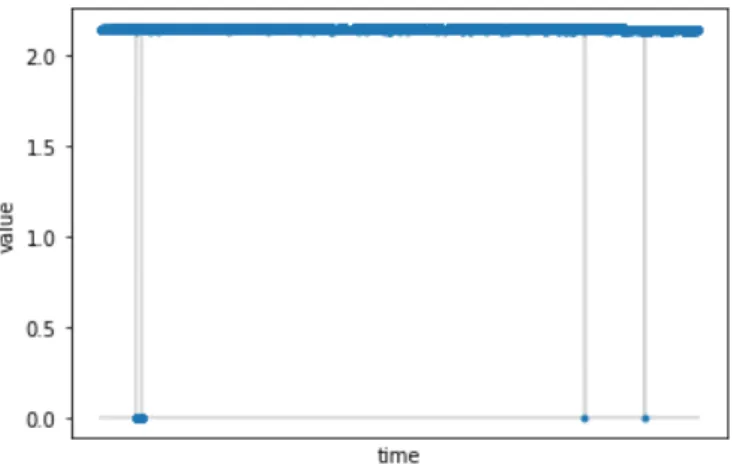
Figure 11 Feature f)

The final noteworthy discovery are features like f). It has seemingly the same value during the whole period, if disregarding the sudden changes during labeled outages plotted as 0. It is acknowledged that the variance of f) could seem more significant if the visualization would not scale down to 0 during outages. This shows another flaw in the outage labeling process, when labeling numerical outages as zero. This type of features could be transformed to better scale, however, in this study they are discarded, since the number of features is already relatedly large. The results of the feature elimination are summarized below:

Feature elimination results:

 Both log and metric features are filtered. Each feature that has issues like a), b), c), e)

or f) are discarded from analysis. The process results in 36 log and 29 metric features (total 65) for dataset 1. For dataset 2, the numbers are 35 for both logs and metrics (total 70).

 A decision is made to shorten the time series of dataset 2, by matching it with the update of API-manager (see fig. 7). There are multiple features of the service that would have needed to be discarded in both datasets because of the update, that are now only discarded from dataset 1.

(42)

4.4.3 Target variable

To apply the final step of feature selection, the target variable must be selected or extracted before. This variable should focus on the 10 main log level features produced by the integration engine in cores1 and 2. The proposed solution is an overall error score variable calculated from each of the logs. This would reflect the state of the whole operation, as errors in a single log would increase the score marginally, whereas errors in all logs would increase it drastically.

As seen in 4.3.3, the individual logs have different minimum and maximum values of severity, some having the latter as fatal and others as error. Therefore, each log level is first given a numerical value representing the severity, and after that, these numbers are standardized by z-score, where each log’s maximum severities are scored highest, and minimum lowest, based on the distribution of severity. It is acknowledged that for some logs, the higher severities could be yet to occur, but this issue is not focused on this study. To prevent corrupting the log level scoring, the outages are disregarded from the output variable, rather than given each log level a score like 0 during them. This is done by imputing missing values with the last occurred severity for each log, like the imputation in 4.3.2. The whole process of error score is presented as algorithm below:

1. iterate log level feature by values (repeat for each log level): if value is 'null':

replace value with last preceding or next following value else if value is not 'null':

replace:

'WARN' by 1 'ERROR' by 2 'FATAL' by 3 others by 0

2. z-score standardize values along each feature

3. concatenate the features into table (1 column/feature). 4. initialize final error score variable as list

5. iterate the concatenated table by rows: count sum of of all values in the row append the sum to error score list

(43)

Figure 12 Initial error score visualization. Dataset 1 (left), dataset 2 (right).

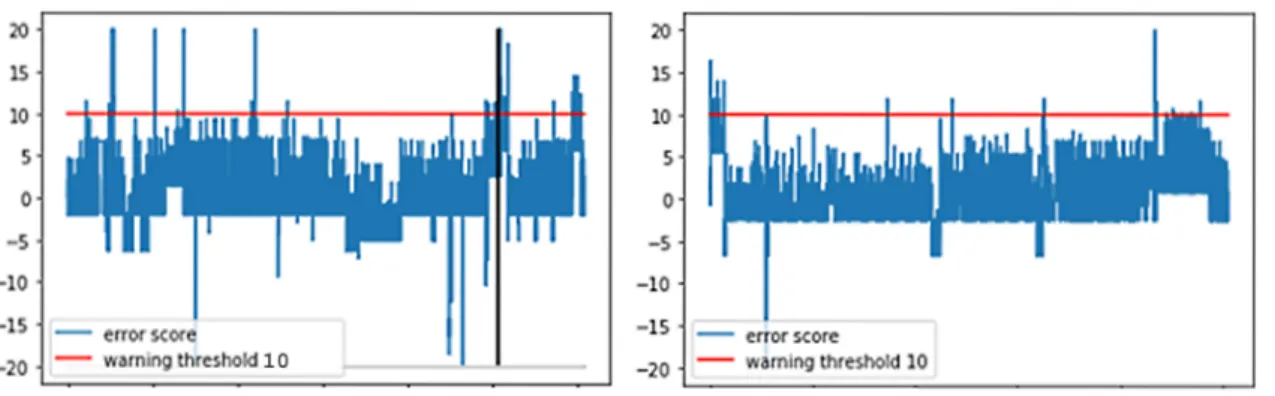
The generated error scores are plotted in fig. 12. With dataset2, the frequency of more severe loggings is very sparse for some logs, which makes their scores very high after standardization. With dataset 1, the variable seems to vary in more stable manner. To avoid the high variance, it is decided to transform all scores higher than 20 to 20 and scores lower than -20 to -20. This smoothens the plot, which makes the predicting better, especially if the forecasting method is easily biased by outliers in data. Although reducing the error scores of the few very high instances, the transformation keeps the score relatively high to trigger a warning, which is essentially the only requirement for the error score. The transformed error scores are plotted in fig. 13. A potential threshold for triggering warnings is visualized as a red line.

Figure 13 Transformed error score visualization. Dataset 1 (left), dataset 2 (right). The black

Big Data Preprocessing for Multivariate Time Series Forecast