Residual Stress Analysis For Axisymmetric Welded Cone & Tee Assembly Model

(1)

Lehigh University

Lehigh Preserve

Theses and Dissertations

2016

Residual Stress Analysis For Axisymmetric Welded

Cone & Tee Assembly Model

Shuoran Du

Lehigh University

Follow this and additional works at:http://preserve.lehigh.edu/etd Part of theMechanical Engineering Commons

This Thesis is brought to you for free and open access by Lehigh Preserve. It has been accepted for inclusion in Theses and Dissertations by an authorized administrator of Lehigh Preserve. For more information, please [email protected].

Recommended Citation

Du, Shuoran, "Residual Stress Analysis For Axisymmetric Welded Cone & Tee Assembly Model" (2016).Theses and Dissertations. 2579.

(2)

Residual Stress Analysis For Axisymmetric Welded

Cone & Tee Assembly Model

by Shuoran Du

A Thesis

Presented to the Graduate & Research Committee of Lehigh University

in Candidacy for the Degree of Master of Science

in

Mechanical Engineering

Lehigh University

April 2016

(3)

ii

This thesis is accepted and approved in partial fulfillment of the requirements for the Master of Science.

Date

Thesis Advisor

(4)

iii

Acknowledgment

Firstly, I desire to express my sincere gratitude to my advisor Professor Herman F. Nied for his patience, immense knowledge and continuous support for my master program study. His help and guidance helped me learn a lot in field of welding simulation and computational mechanics. In addition, my sincere thanks also goes to my colleague Dr. Tianyi Luo for the simulating discussions. I also thank Mr. Muhammed Ashraf for helping me deal with problems of workstation. Last but not least, I would like thank my parents for their encouragement and support for my master study.

(5)

iv

List of Figures

Figure 1.1 Parts idagram of Cone & Tee Assembly Model ... 4

Figure 1.2 Work flow of FEA simulation for this study ... 5

Figure 2.1 Fully Cone & Tee Assembly Model with rotation symmetry axis ... 6

Figure 2.2 2-D axisymmetric Cone & Tee Assembly Model ... 7

Figure 2.3 Close-up view of 2D axisymmetric model with different number of weld pass: ... 8

Figure 2.4 2D finite elements used :(a) Quadratic 2-dimensional element for components of model (b) Quadratic-triangular mixed mesh for welded filler ... 9

Figure 2.5 1-dimension elements used for heat transfer boundary condition ... 9

Figure 2.6 Welding components and fillers of model:... 10

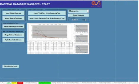
Figure 2.7 Material Database Manager of SYSWELD ... 13

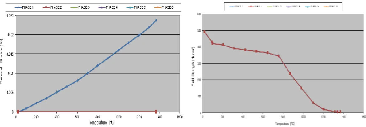
Figure 2.8 Critical properties of Incoloy 800HT for welding simulation in different temperatures: (a) Thermal conductivity (𝑊/𝑚℃) (b) Young’s Modulus (𝑀𝑝𝑎) (c) Thermal Strains (d) Yield Strength (𝑀𝑝𝑎) ... 14

Figure 2.9 Critical properties of Inconel 617 for welding simulation in different temperatures: (a) Thermal conductivity (𝑊/𝑚℃) (b) Young’s Modulus (𝑀𝑝𝑎) (c) Thermal Strains (d) Yield Strength (𝑀𝑝𝑎) ... 15

Figure 2.10 Boundary condition 1 ... 15

Figure 3.1 Global Parameter for welding simulation ... 18

Figure 3.2 Double ellipsoid model of ARC power resource... 19

(8)

vii

Figure 3.4 Geometry of weld pool ... 20

Figure 3.5 Cooling condition setting... 21

Figure 4.1 Temperature contours for each weld pass in 1 weld passes simulation: ... 23

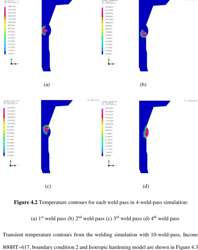
Figure 4.2 Temperature contours for each weld pass in 4-weld-pass simulation: ... 24

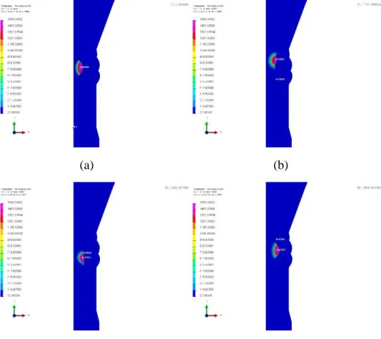
Figure 4.3 Temperature contours for each weld pass in 10-weld-pass simulation: ... 26

Figure 4.4 Temperature changes with time in nodes of HAZ and non HAZ: ... 27

Figure 4.5 Temperature contours for each weld pass in 20 weld passes simulation: ... 30

Figure 4.6 Overall von-Mises stress distribution comparison for different number of weld pass (a) 1 weld pass (b) 4 weld passes (c) 10 weld passes (d) 20 weld passes ... 32

Figure 4.7 Von-Mises stress distribution in HAZ: ... 34

Figure 4.8 Von- Mises stress comparison on surface A-B for different number of weld pass simulations: (a) Position of surface A-B (b) Stress distribution on surface A-B... 36

Figure 4.9 Von-Mises stress comparison on surface A-C for different number of weld pass simulations ... 37

Figure 4.10 Von-Mises stress comparison on internal surface for different number of weld pass simulation: (a) Position of internal surface (b) Stress distribution on internal surface ... 39

Figure 4.11 Von-Mises stress comparison on surface E-F for different number of weld pass simulation ... 40

Figure 4.12𝜎𝑦𝑦 stress distribution comparison for different number of weld pass (a) 1 weld pass (b) 4 weld passes (c) 10 weld passes (d) 20 weld passes ... 42

Figure 4.13𝜎𝑦𝑦 stress comparison on section G-H for different number of weld pass simulations ... 43

(9)

viii

Figure 4.14𝜎𝑦𝑦 stress comparison on top surface for different number of weld pass simulations ... 44 Figure 4.15𝜎𝑧𝑧 stress distribution comparison for different number of weld pass: ... 45 Figure 4.16𝜎𝑧𝑧 stress comparison on internal surface for different number of weld pass: (a) Position of internal surface (b) Stress distribution on internal surface ... 46 Figure 4.17 Overall Von-Mises stress distribution comparison for different material: ... 47 Figure 4.18 Plastic strain distribution comparison: (a) 316L (b) Incoloy 800 HT + Inconel 617 48 Figure 4.19 Von-Mises stress comparison on selected surfaces for simulations with different material (a) Surface A-B (b) Section A-C ... 49 Figure 4.20 Material property comparison for three different material: (a) Product of Young’s modulus and coefficient of thermal expansion (b) Yield stress ... 51 Figure 4.21𝜎𝑧𝑧 stress overall distribution comparison for simulations with different material: (a) 316L (b) Incoloy 800 HT + Inconel 617 ... 52 Figure 4.22𝜎𝑦𝑦 stress comparison on section E-I ... 52 Figure 4.23𝜎𝑦𝑦 stress on selected surfaces for simulations with different material group: ... 54 Figure 4.24𝜎𝑧𝑧 stress distribution comparison for simulations with different material: (a) 316L (b) Incoloy 800 HT + Inconel 617 ... 55 Figure 4.25𝜎𝑧𝑧 stress comparison on section A-C and J-K: ... 57 Figure 4.26𝜎𝑧𝑧 stress distribution on internal surface ... 57 Figure 4.27 Overall Von-Mises stress distribution comparison for different Boundary

Conditions: ... 59 Figure 4.28 von- Mises stress comparison on external surface from Node B to bottom edge .... 60 Figure 4.29𝜎𝑦𝑦 stress distribution comparison for different Boundary Conditions:... 62

(10)

ix

Figure 4.30𝜎𝑧𝑧 stress distribution comparison for different Boundary Conditions: ... 63

Figure 4.31𝜎𝑦𝑦 stress and 𝜎𝑧𝑧 stress comparison on surface M-N ... 64

Figure 5.1 Stress-strain curve of isotropic hardening [24]: (a) Uniaxial (b) Multiaxial ... 66

Figure 5.2 Stress-strain curve of kinematic hardening: (a) Uniaxial (b) Biaxial ... 67

Figure 5.3 MDM labels of plastic hardening model ... 68

Figure 5.4 Overall Von-Mises stress distribution comparison for different plastic hardening model: (a) Isotropic hardening (b) Kinematic hardening ... 70

Figure 5.5 Von-Mises stress distribution comparison in the HAZ for different plastic hardening models: (a) Isotropic hardening (b) Kinematic hardening ... 72

Figure 5.6 Von-Mises stress comparison on surface E-F for different plastic hardening model 72 Figure 5.7 Von-Mises stress comparison on section A-C for different plastic hardening model 74 Figure 5.8 Von-Mises stress comparison on internal surface for different plastic hardening model... 74

Figure 5.9 Von-Mises stress at Node E changes with time for different plastic hardening model ... 76

Figure 5.10 Von-Mises stress of Node P changes with time for different plastic hardening model ... 77

Figure 5.11 Von-Mises stress of Node Q changes with time for different plastic hardening model ... 78

(11)

x

List of Tables

Table 2.1 Chemical composition of 316L ... 11 Table 2.2 Chemical composition of Incoloy 800HT ... 11 Table 2.3 Chemical composition of Inconel 617 ... 12

(12)

1

Abstract

Residual stresses are generated from the non-linear thermal loading and unloading cycles that occur during a typical multi-pass ARC welding process. Large residual stresses and plastic strains will in turn cause reliability problems closely associated with cracking and distortion in welded structures, which will ultimately reduce the structure’s fatigue life. In this study, the particular structure of interest is an outlet manifold fabricated with large circumferential welds. SYSWELD is used to simulate the welding process of the Cone and Tee weld in the outlet manifold using four numbers of weld passes (1 weld pass, 4 weld passes, 10 weld passes and 20 weld passes) and two different material groups (Group 1: Incoloy 800 HT for base alloy and Inconel 617 for filler metal, Group 2: 316L for both base alloy and filler metal), three different boundary conditions and two different plasticity model (Isotropic hardening and kinematic hardening). By using Finite Element Analysis and comparison analysis with varying singular welding process parameter, the influence of different numbers of weld passes, materials, boundary conditions and plasticity models on the residual stress distribution can be found. It is shown that the number of welded passes has significant influence on the residual stress distribution. The simulation results also indicate that the Inconel alloy group and the 316L materials will give rise to similar plastic deformation zones, but different stress value in the same positions. Additionally, the boundary conditions lead to localized residual stress concentrations in area near rigid clamped conditions. Isotropic and kinematic plasticity models result in slightly differences on stress values of plastic deformation areas and are also discussed in detail in this study.

(13)

2

Chapter 1 Introduction

Arc welding is one commonly used fusion welding process in industrial manufacturing projects. In the welding process, an intense heat source is used to melt and join components and welded filler metals in order to make a molten fusion bond [1]. The temperature of areas near the welding arc are on the order of one thousand degree Celsius. The large heat energy generated during welding is conducted into the bulk of metal as the welding process proceeds. In multi-pass welding, the welding arc will repetitively create nonlinear thermal loading and cooling cycles. Welding is a complicated process which will induce volumetric changes producing transient and residual stresses and deformation [2-4]. Thermal deformation companied by thermal strains mainly exists in the welded fillers and contiguous areas. Areas with sufficiently large Von Mises strains will deform plastically.

Residual strains can cause problems for welded structures during utilization. Accumulating distortion and initiation of cracks will reduce the welded structure’s quality of fit and reliability. Residual stress resulting from nonlinear thermal cycles in welding produces internal forces that cause a variety of problems [5]. It is a main factor for crack initiation and crack growth in the welded structures during cooling [6]. There are two forces in the cooling process: stress resulting from non-uniform shrinkage due to thermal gradients and stress that arises from surrounding boundary condition constraints. Because the contraction is restricted, the strain will cause residual stress [7-8]. Because of large size of the structure, there is a large amount of constraint that causes highly localized residual stresses in the neighborhood of welds.

(14)

3

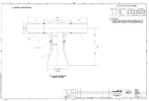
The outlet manifold focused in this study is a Cone & Tee Assembly as shown in Fig. 1. Pressure and corrosion of gas is known to accelerate cracking in the presence of high residual stresses. The presence of welding residual tensile stresses in the heat-affected zone (HAZ) may accelerate the corrosion attack and enhance cracking, particularly along sensitized grain boundaries [9-10]. Hence, welding stress analysis for the Cone & Tee Assembly model is necessary in order to reduce the likelihood of failure.

Because of the large influence the residual stresses have on reliability of welded structures, there are numerous assessments methods for residual stress measurements and analysis methodology. Most common residual stress measurement methods can be divided by two types. (1) Mechanical invasive methods, such as hole drilling or cutting. (2) Non-destructive methods, such as X-ray and neutron diffraction [11]. Alternatively, computational residual stress analysis techniques have become highly developed and are very useful for examining how specific welding parameters affect the final residual stress state.

In this study, residual stress comparisons are generated based on finite element analysis for the Cone & Tee assembly geometry with different numbers of welded passes, alloys, boundary conditions and plastic hardening models. The total height of model is about 49.75 inches and the external diameter is 16.00 inches (see Figure 1.1). Because the model is relatively large and many different welding conditions need to be examined, experimental

(15)

4

residual stress techniques are economically infeasible. The FEA simulations are particularly useful in depicting the time evolution of the welding process, permitting a detailed visualization of material deformation and stresses.

Figure 1.1 Parts idagram of Cone & Tee Assembly Model

Currently, several commercial CAE software packages can be used to simulate the transient temperature and stress distribution in welding processes. SYSWELD [12] is used for this study. SYSWELD is a non-linear finite element code specifically designed for solving welding problems. SYSWELD was created from the SYSTUS system for the nuclear industry in 1981 and has been under continuous development for over forty-five years. SYSWELD couples calculation for heat transfer, material properties and

mechanical behavior of model, taking into account phase transformations have on temperature distribution [13]. These calculations are performed sequentially in the order: Thermal, Metallurgy, Mechanical. In the process of calculating mechanics, residual stresses for the unclamped condition can be got in SYSWELD by releasing boundary conditions at last second of simulation [14].

(16)

5

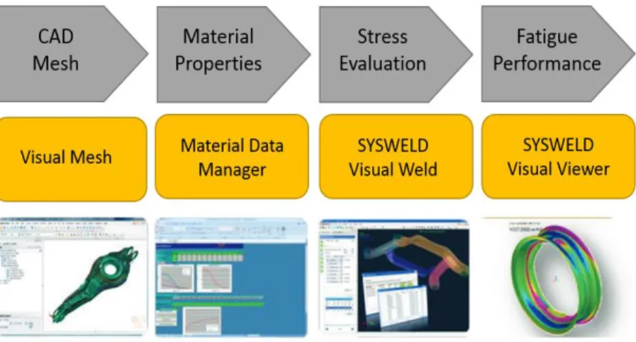
Visual Environment 10.5 as the graphical interface used with SYSWELD. Not only it is easy to use, but Visual Environment also encompasses many non-linear finite element analysis software tools designed for some specific problems such as Visual- Quoting, Visual- CFD. In this study, Visual- Mesh 10.5, Visual- Weld 10.5 and Visual- Viewer 10.5 are used. These three packages cover all the functions needed for the welding simulation planner and designer. In this study, Visual- Mesh [15] is used to edit CAD models, create 2D meshes, automatically clean up surfaces, check and correct mesh quality and assembly. Visual- Weld [16] is a welding & heat treatment simulation tool which is for welding process design. Furthermore, Visual- Viewer [17] is used to post process FE analysis data, create video animations and plot data. Figure 1.1 shows the work flow of the SYSWELD software used in this study.

(17)

6

Chapter 2 Weld Process Simulation Model

2.1 Modeling

Figure 2.1 is the 2-dimensional fully Cone & Tee Assembly Model with rotation symmetry axis studied in this research. The total height of the cone section is 0.679m (26.75 inches), and the height of the tee is about 0.584m (23 inches). In this study, we have focused on the welded sections which join the lower Cone structure (Blue part in Figure 2.1) to the upper Tee structure (Yellow part in Figure 2.1). The distance between the horizontal central line of the weld filler and the bottom of horizontal cylinder of the tee is 0.159m (6.25 inches). During welding, very little heat can transfer to upper part of the tee. Furthermore, besides convection to the air, there is also heat conduction with the lower part of the tee that can be ignored in simulation and its upper part. So the finite element model only includes the entire cone section and only the vertical pipe of the tee and cone. Two pipes shown as item 3 in Figure 2.1 and upper horizontal pipe of the tee are omitted in the analysis.

(18)

7

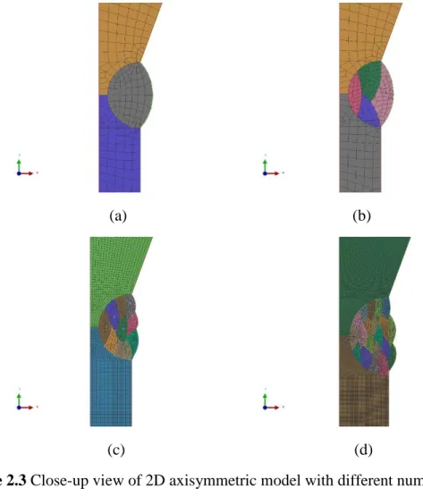
In this problem, a 2D rotational axisymmetric model is used for the Finite Element Analysis, shown as Figure 2.2 which is the right part of fully Cone & Tee Assembly model of Figure 2.1. Main difference between a full 3D model and a 2D axisymmetric model is the thermal and mechanical results at the beginning and end time of the welding process. In a full 3D weld simulation the heat source center moves with a specific velocity. While in the axisymmetric model, the heat source doesn’t actually move, but instead uniformly increases and decreases at all points as a specific function of time. Hence it’s expected that the residual stresses will be the same except perhaps where the welding starts and stops in the fully 3D case. Because of the high computational efficiency, the 2D axisymmetric model was chosen for solving the circumferential welding problem. Figure 2.2 depicts the meshed axisymmetric 1 weld pass model, 4 weld passes model, 10 weld passes model and 20 weld passes model of outlet manifold with their welding lines and reference lines. 2D axisymmetric model is built on x-y plane. In each figure, the tee component and cone are in different colors.

(19)

8

(a) (b)

(c) (d)

Figure 2.3 Close-up view of 2D axisymmetric model with different number of weld pass: (a) 1 weld pass (b) 4 weld passes (c) 10 weld passes (d) 20 weld passes

2.2 Meshing

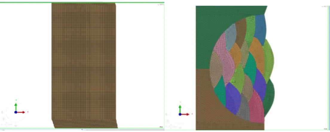
After the rotational axisymmetric geometric models are built, they are meshed in Visual-mesh 10.5 [15]. The main Visual-mesh element type is the quadratic 2-dimensional element shown in Figure.2.3 (a). And the mesh method is pave. For some welding filler parts in irregular form, it is difficult to generate Quads mesh. So both the quadratic element and triangular element type should be used, as shown in the weld beads for the 20 weld pass model in Figure 2.3 (b).

(20)

9

(a) (b)

Figure 2.4 2D finite elements used :(a) Quadratic 2-dimensional element for components of model (b) Quadratic-triangular mixed mesh for welded filler

For the heat transfer boundary condition between solid and air of the 2D model, 1-dimension elements are used as shown by the red lines in Figure 2.4.

(21)

10

2.3 Materials

There are three kinds of metals used in this this study- 316L stainless steel, Incoloy 800HT and Inconel 617. One material group includes Incoloy 800HT for welding components shown as the red part in Figure 2.5 (a), and Inconel 617 as the welding filler material shown as Figure 2.5 (b). While 316L for both upper and lower welding components and welding filler material is used to compare residual stresses with simulation using Inconel alloy group above.

(a) (b)

Figure 2.6Welding components and fillers of model: (a) Welding components (b) Welding fillers

316L stainless steel is a typical austenitic chromium nickel stainless steel, which can minimize harmful carbide precipitate due to welding and provides optimum corrosion resistance [20]. Table 3.1 shows the chemical composition of 316L.

(22)

11

Table 2.1 Chemical composition of 316L

C% Max Mn% Max P% Max S% Max Si% Max

Cr% Ni% Mo% Ni%

Max

Iron

0.03 2 0.045 0.03 0.75 16-18 10-14 2-3 0.1 Balance

Incoloy 800HT or Inconel 800HT has a high creep and rupture strength. Because of its excellent mechanical properties combined with high resistance to high-temperature corrosion, it is widely used to make outlet manifolds where heated gas pass though. It has the same chemical element with the Incoloy 800 and 800H, but the carbon content is restricted to 0.06-0.10% and Al+ Ti content is restricted to 0.85-1.20%. Incoloy 800HT has good resistance to high temperature corrosion and good weldability [21]. Table 3.2 shows the chemical composition of Incoloy 800HT.

Table 2.2 Chemical composition of Incoloy 800HT

Ni% Cr% Iron%

Min

C% Al% Ti% Al%+Ti% ASTM

Grain size

30-35 19-23 39.5 0.06-0.10 0.25-0.60 0.25-0.60 0.85-1.20 5 or coarser

Inconel 617 is a high-temperature strength and oxidation resistance nickel-chromium-cobalt-molybdenum alloy. It has excellent mechanical properties in a large range of

(23)

12

temperature especially its resistance to corrosion in high temperature. Table 3.3 shows the chemical composition of Inconel 617.

Table 2.3 Chemical composition of Inconel 617

Ni%

Min

Cr% Co% Mo% Al% C% Iron%

Max Mg% Max Si% Max S% Max Ti% Max Cu% Max B% Max 44.5 20-24 10-15 8-10 0.8-1.5 0.05-0.15 3.0 1.0 1.0 0.015 0.6 0.5 0.006

Both Incoloy 800HT and Inconel 617 have excellent weldability. Because of high creep-rupture strength, Incoloy 800HT should be joined upon the intended service temperature. And Inconel 617 is widely used as filler metal in many welding projects. Inconel 617 filler metal has a much higher yield stress and greater tensile strength when compared to Inconel alloy 182 and Inconel alloy 600.

In SYSWELD, the 316L material database is contained in the Visual-weld public material database. But because there are no Incoloy 800HT and Inconel 617 material databases in SYSWELD, these two material property databases needed to be built using the Material Database Manager (MDM) [18] from the SYSWELD Welding Tool Box 2015 shown in Figure 2.6. The database of each kind of alloy has two subset databases: 1) Thermo-Metallurgy database, and 2) Mechanics database. The main thermal and mechanical properties of Inconel Alloy needed for welding simulation are thermal conductivity, Young

(24)

13

Modulus, Poisson’s Ratio, Thermal Strain, Yield stress and Strain Hardening. In this study, the thermal and mechanical properties of Incoloy 800HT and Inconel Alloy 617 that were put into the SYSWELD database mentioned above were obtained from [21] and [22].

Figure 2.7 Material Database Manager of SYSWELD

The mean Poisson’s Ratio in the database of Inconel alloys are set as the constant independent to the temperatures for SYSWELD. The Fig 2.7 and Fig 2.8 respectively shows the Thermal Conductivity, Young’s Modulus, Thermal Strains and Yield Strength of Incoloy 800 HT and Inconel 617 as a function of temperature.

(25)

14

(c) (d)

Figure 2.8 Critical properties of Incoloy 800HT for welding simulation in different

temperatures: (a) Thermal conductivity (𝑊/𝑚℃) (b) Young’s Modulus (𝑀𝑝𝑎) (c)

Thermal Strains (d) Yield Strength (𝑀𝑝𝑎)

(26)

15

(c) (d)

Figure 2.9 Critical properties of Inconel 617 for welding simulation in different

temperatures: (a) Thermal conductivity (𝑊/𝑚℃) (b) Young’s Modulus (𝑀𝑝𝑎) (c)

Thermal Strains (d) Yield Strength (𝑀𝑝𝑎)

2.4 Boundary Conditions

There are 3 kinds of boundary conditions considered in this study. These 3 boundary conditions are defined through the Visual-Weld 10.5 interface. In Figure 2.9, for Boundary condition 1, Rigid clamped conditions in X, Y, Z directions are set for nodes on the top edge.

(27)

16

Boundary condition 2 is shown in Figure 2.10: Rigid clamped conditions in the Y direction is set for nodes on the top surface of the model, and Rigid clamped conditions in the X and Z directions are set for the 1st node on top edge. Rigid clamped conditions in Y and Z directions are set for the nodes on bottom edge, after the component has completely cooled, unclamped conditions are specified for nodes on bottom edge.

(a) (b)

Figure 2.11 Boundary condition 2

(a) Before the component has completely cooled (b) After the component has completely cooled

Boundary Condition 3 (Figure 2.11): Rigid clamped conditions in Y direction is set for nodes on top surface of the model, and Rigid clamped conditions in X and Z directions are set for the 1st_{node on top edge. No boundary condition constrained are set for the nodes}

(28)

17

Figure 2.12 Boundary condition 3

In general, Boundary condition 1 and Boundary condition 3 have the same clamped conditions along the bottom edge. And Boundary condition 2 and Boundary condition 3 have the same clamped conditions on the top surface and top edge.

For heat transfer boundary conditions in this problem, heat transfer from the 2D axisymmetric Tee & Cone Assembly model with the environment is through Newtonian heat convection. Because of large radius of cone part and tee’s upper pipe, the air inside the cone and tee assembly model can be regarded as surrounding air. Hence, heat transfer conditions set for internal surface are the same with external surface shown as Figure 2.4.

(29)

18

Chapter 3 Settings for welding simulation

After the model is built and the mesh is generated in Visual-Mesh 10.5, Visual-Weld 10.5 is used to define the appropriate parameters for the welding simulations.

3.1 Global Parameter

In this study, the computation global parameter is set as 2D rotational, because all the weld passes are along the external surface of the cone and tee model, described as a time dependent axisymmetric model.

Figure 3.1 Global Parameter for welding simulation

3.2 Welding Process Settings

There are some common settings for all the simulations. The process type is General ARC. Figure 3.2 shows the dimension of double ellipsoid ARC power source model in Visual

(30)

19

weld. The welding velocity used is 6.329 mm/sec. Efficiency is 1.000. Power ratio is 1.200. And length ratio is 0.500 [19].

Figure 3.2 Double ellipsoid model of ARC power resource

(a) (b)

Figure 3.3 Welding process settings: (a) weld pool (b) Energy

For simulations with the same number of weld passes, the length, width, penetration and energy per unit length for identical weld passes in different simulations are same. For weld pass simulations with different numbers of welds, these geometry parameters are different in order to make entire weld cross-section heat above metal’s melting point. Figure 3.3

(31)

20

shows settings for weld fillers in weld advisor of Visual-weld 10.5. And Figure 3.4 shows the dimension parameters of weld pool.

Figure 3.4 Geometry of weld pool

3.3 Cooling Condition Setting

Cooling medium used in this study is Free Air Cooling and the ambient temperature is

20℃. The cooling time shown in Figure 3.5 equals the entire simulation time. Because

models with different numbers of weld passes, have different times for welding and cooling, the totally simulation time is different. The model should have enough time-steps to cool down to ambient temperature. For 1-weld–pass model, the simulation time was 25001s. The simulation time for a 4-weld-pass model was set as 27501s. The simulation time for a 10-weld-pass model was 25001s. And the simulation time for the 20-weld-pass model was 35001s.

(32)

21

Figure 3.5 Cooling condition setting

There are no additional loads, deformation settings and contact definition settings for the simulations in this study.

(33)

22

Chapter 4 Welding simulation results

4.1 Heat Transfer Behavior

Transient temperature contours from the welding simulation with 1-weld-pass, Inconel 800HT+617, boundary condition 2 and Isotropic hardening model are shown in Figure 4.1. Isotropic model implies the yield strength in tension and compression stress state are the same for alternating tensile and compressive loading , which will be discussed in Chapter 5 in details. Heat from deposited weld filler metal transfers to other parts of model during the cooling process. Because size of the welded filler is large, much more energy need to heat the entire weld filler than other models. Hence it also need for more time to be completely cooled. At 3.16s, weld bead has finished welding and released all heat resource to the model. At about 25000s, the entire model completely cools to surrounding temperature. Thus, the cooling time is about 24997s. But from 4-weld-pass simulation, the cooling time from last weld bead finish heating to completely cooling is about 23497s. The cooling time of 10-weld-pass simulation is about 11499s. And the cooling time of 20-weld-pass simulation is about 5400s.

(34)

23

(a) (b)

(c) (d)

Figure 4.1 Temperature contours for each weld pass in 1 weld passes simulation:

(1) t= 3.16s (2) t= 93.02s (3) t= 233.01s (4) t=1894.46s

Transient temperature contours from the welding simulation with 4-weld-pass, Inconel 800HT+617, boundary condition 2 and Isotropic hardening model are shown in Figure 4.2. In multi-pass welding simulation, the entire weld metal is part of the model during welding process even when the first weld bead is deposited. For example, in Figure 4.2 (a) first weld bead, the other weld pass fillers are still not activated. So heat flux is only conducted to base metal. In Figure 4.2 (b), only the first two weld beads are activated. The heat flux at this time period is conducted to base metal and the first weld bead. Until the heat source of last weld bead begins to work, the entire weld metal model is activated shown as Figure 4.2 (d).

(35)

24

(a) (b)

(c) (d)

Figure 4.2 Temperature contours for each weld pass in 4-weld-pass simulation:

(a) 1st weld pass (b) 2nd weld pass (c) 3rd weld pass (d) 4th weld pass

Transient temperature contours from the welding simulation with 10-weld-pass, Inconel 800HT+617, boundary condition 2 and Isotropic hardening model are shown in Figure 4.3. Different with 1 weld pass and 4 weld pass simulation, since the area of each weld pass is relatively small compared to the cross-sectional area of the entire Cone & Tee Assembly Model, the heating is quite localized on the nearby area called Heat Affect Zone (‘HAZ’).

(36)

25

Areas near the boundaries and far away from the HAZ, are not affected by heat from welding process in to any significant degree. This conclusion can be seen in Figure 4.4 which the temperature of a node located in the HAZ (Node 150) with another node (Node 1346) not in the HAZ changes as a function of time. The distance between the two picked nodes are 203.5434 mm.

(a) (b)

(37)

26

(e) (f)

(g) (h)

(i) (j)

Figure 4.3 Temperature contours for each weld pass in 10-weld-pass simulation:

(a) 1st weld pass (b) 2nd weld pass (c) 3rd weld pass (d) 4th weld pass (e) 5th weld pass (f) 6th weld pass (g) 7th weld pass (h) 8th weld pass (i) 9th weld pass (j) 10th weld pass

(38)

27

(a) (b)

Figure 4.4 Temperature changes with time in nodes of HAZ and non HAZ: (a) Position of Node 150 and Node 1346 (b) Transient temperature of Node 150 and

Node 1346 in welding process

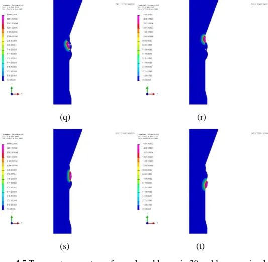
Figure 4.5 is transient temperature contours from the welding simulation with 20-weld-pass, Inconel 800HT+617, boundary condition 2 and Isotropic hardening model. Similar with 10-weld-pass simulation, because of limited size of each weld filler, area far away from the HAZ are not affected by heat from welding process in to any significant degree in 20-weld-weld pass simulation.

(a) (b)

(39)

28

(e) (f)

(g) (h)

(40)

29

(k) (l)

(m) (n)

(41)

30

(q) (r)

(s) (t)

Figure 4.5 Temperature contours for each weld pass in 20 weld passes simulation:

(a) 1st weld pass (b) 2nd weld pass (c) 3rd weld pass (d) 4th weld pass (e) 5th weld pass (f) 6th weld pass (g) 7th weld pass (h) 8th weld pass (i) 9th weld pass (j) 10th weld pass (k) 11th weld pass (l) 12th weld pass (m) 13th weld pass (n) 14th weld pass (o) 15th weld pass

(p) 16th weld pass (q) 17th weld pass (r) 18th weld pass (s) 19th weld pass (t) 20th weld pass

4.2 Residual stress analysis

In this section, the residual stress distribution from simulations with different numbers of weld passes, material groups and boundary conditions are compared and analyzed in order to find the influence of these factors on the residual stress distribution. Furthermore, local

(42)

31

horizontal and vertical residual stress component distributions are plotted along continuous lines.

4.21 Residual Stress comparison for simulations with different numbers of weld passes

Figure 4.6 shows the Von-Mises stress distribution from simulations with 1 weld pass, 4 weld passes, 10 weld passes and 20 weld passes. All the simulations in this section have the same material group (Incoloy 800HT+ Inconel 617), boundary conditions (Boundary condition 2) and plastic hardening model (Isotropic hardening). The temperature scale for all four of these pictures are the same. Thus, areas with the same color represent the same range of von Mises stress. A cut-off value of the color contours was used so that red areas in these contours represent where von-Mises Stress is larger than the uniaxial yield stress of Incoloy 800HT which is about 241.32 MPa at 21℃ . Additionally, pink areas in these pictures represent where the von-Mises Stress is greater than the uniaxial yield stress of Inconel 617 which is about 340 MPa at 21℃ .

(43)

32

(c) (d)

Figure 4.6 Overall von-Mises stress distribution comparison for different number of weld pass (a) 1 weld pass (b) 4 weld passes (c) 10 weld passes (d) 20 weld passes

From results comparison of Figure 4.6, it can be seen that the plastic deformation area in a 1 weld pass simulation in Figure 4.6 (a) is much larger than that obtained from the other three multi-pass simulations in Figure 4.6 (b) (c) (d). Because the total height of Cone & Tee assembly model is 1200.15mm (47.25 inches) and the height of the zone filled with weld metal studied is about 81.47mm, in reality, it is not possible to use just 1 weld pass to join such two large components. Hence, a 1 weld pass simulation for this problem can’t realistically describe the stress distribution in an actual Cone & Tee Assembly. However, the single weld pass model does serve as a baseline for comparison with the more realistic multi-pass simulation models. It’s interesting to note that von-Mises stress distributions shown in Figures 4.6 (b), (c) and (d) are remarkably similar, especially in the areas outside of the multi-weld fusion zone.

(44)

33

Von-Mises Stress distributions in the HAZ for different numbers of weld pass simulations are shown in Figure 4.7. Comparing Figure 4.4 (b) with (c) and (d), the plastic deformation area from a 4 weld pass simulation are larger than that seen in the 10 weld pass and 20 weld pass simulations, especially in the area near the external surfaces of the Tee and cone. Von-Mises stress distributions of 10 weld passes and 20 weld passes in Figure 4.7 (c) and (d) are quite similar everywhere the model. The maximum von Mises stresses in the model with 10 weld passes and 20 weld passes are 469.510 MPa and 467.092 MPa. Values and positions of the max stress nodes are nearly the same in these two multi-pass weld simulations.

(45)

34

(c) (d)

Figure 4.7 Von-Mises stress distribution in HAZ:

(a) 1 weld pass (b) 4 weld passes (c) 10 weld passes (d) 20 weld passes

Distributions of von-Mises stress and stress components on some surfaces chosen are compared below, in order to discuss the influence of different numbers of weld pass has on residual stress.

Figure 4.8 (a) shows the position of surface from A to B which is a part of external surface of cone. Node A is the node in the corner between welded filler metals and the external surface of Cone part. Node B is the node on the intersection line of the cylindrical surface and circular conical surface of the cone. Figure 4.8 (b) shows a comparison of von-Mises Stress distribution of different weld pass numbers simulation on surface A-B. According to this figure, there are two stress concentration nodes, which is a node near node A and the node 100 mm away from node A designated as Node G in Figure 4.8 (a). Node G is the corner of the small beveling of the cone. The von-Mises Stress (stress concentration) near node A is about 300 MPa, and Von-Mises stress of the other stress concentration node is about 250 MPa. The black curve and green curve are similar especially in the area 100 mm away from node A to node B. In this area, the von-Mises stress of 1 weld pass simulation (blue curve) does not decrease. Whereas, stresses from the 4 weld passes simulation (red curve) decreases to some degree but not as large as that seen in the simulations using 10 weld passes and 20 weld passes. In the area from node A to the node 100 mm away from node A, all the stress results decrease beginning at the node about 30 mm away from node

(46)

35

A and then increase. From 1 weld pass simulation to 20 weld passes simulation, the change degree of stress value becomes lower.

(a)

(47)

36

Figure 4.8 Von- Mises stress comparison on surface A-B for different number of weld pass simulations: (a) Position of surface A-B (b) Stress distribution on surface A-B

Figure 4.9 shows another section chosen for plotting a comparison of the von-Mises stresses. Node C is the node on internal surface of the model with the same height of node A. From Figure 4.9, it is easy to see that except for the 1 weld pass simulation (blue curve), the other multi-pass weld simulations seem to reasonably describe the overall stress trends in this section, i.e. the von-Mises stress declines by about 57.5% from A to C. This section is near the welded filler metal in the heat affect zone. In different numbers of weld passes simulations, different number of heating cycles and the energy mount released by related weld beads will affect the residual stress distribution of section A-C to significant degree. In 1 weld pass simulation, there is just one heating cycle to the entire model. And the total energy released by the only weld filler is very large. In 4 weld pass, the 2nd weld pass and the 4th weld pass are nearest to section A-C, thus there are two heating cycles affecting residual stress of section A-C significantly. And energy released by each weld bead is smaller than 1-weld-pass simulation. While in 10 weld pass, there are three heating cycles affecting residual stress of section A-C significantly because the 2nd, 5th and 8th weld passes are nearest to A-C. For 20 weld pass, the number of heating cycles affecting residual stress reaches 5. The size of each weld pass and energy released is smallest. This is the reason why the difference of curves in Figure 4.9 are so large that easy to be seen.

(48)

37

Figure 4.9 Von-Mises stress comparison on surface A-C for different number of weld pass simulations

Von-Mises Stress distribution along the internal surface of Cone & Tee Assembly Model is shown in Figure 4.10 (b). All the simulations can show the stress concentration node designated as Node L which is about 225mm away from the 1st node of top surface (Node D). This area on the internal surface is located at the same vertical position as the weld on the external surface. From this plot, it can be seen that the stress curves from the 10 weld pass simulation (Green curve) and 20 weld pass simulation (Black curve) are similar. The 1 weld pass simulation only roughly describes the stress distribution along the internal surface. And for Node M shown in Figure 4.10 (a) and (b), the low stress node which is about 200 mm away from node D, 1 weld pass simulation can’t calculate the exact value

(49)

38

just as the other three simulations. The stress value in this area is more than 300 MPa. But the value obtained from the other three multi-pass welding simulations is about 60 MPa. According to Figure 4.10 (b), there are one main plastically deformed areas on the internal surface, an area about 210mm to 240 mm away from Node D shown in Figure 4.10 (b). Zones far away from the deposited welds have low stresses and elastic deformations.

(50)

39 (b)

Figure 4.10 Von-Mises stress comparison on internal surface for different number of weld pass simulation: (a) Position of internal surface (b) Stress distribution on internal

surface

Figure 4.11 shows the position of surface E-F which is a part of tee’s external surface and von-Mises Stress distribution along surface E-F. From Figure 4.11, Node E is the node of joint between welded fillers and external surface of the tee. Node F is the intersection point between the upper pipe and vertical pipe of tee shown in Figure 4.11. Area near node E has stress concentration. Stress values of this area from 4 weld passes, 10 weld passes and 20 weld passes are about 265 MPa. While the stress value from 1-weld-pass simulation is about 350 MPa which is not precise. Furthermore, there is a plastic deformation area beginning at 25 mm away from Node E. Its stress value is about 250 MPa. From

(51)

1-weld-40

pass to 20-weld-pass simulations, the length of the plastic deformation zone decreases. For example, the length of the plastic deformation area in the 4-weld-pass model is about 107 mm. The length of plastic deformation in the 10 weld pass simulation area is about 55 mm. While the length of plastic deformation zone in the 20-weld-pass simulation is just 43mm.

Figure 4.11 Von-Mises stress comparison on surface E-F for different number of weld pass simulation

Figure 4.12 shows the 𝜎_𝑦𝑦stress (stress in vertical direction) distribution for different numbers of weld passes. Similarly with von-Mises stress distributions, the values and area of plastic deformation from the 1-weld-pass simulation is much larger than that obtained from the other three multi-pass models. Thus, the single weld pass model is the only useful for comparison purpose. The 10-weld-pass and 20-weld-pass simulations are very similar,

(52)

41

even the vertical stress distribution 𝜎𝑦𝑦 in the welded filler metals. For the 4-weld-pass

simulation, 10-weld-pass simulation and 20-weld-pass simulation, the maximum vertical stress nodes are all near node E seen in Figure 4.12. But the values of maximum stress from simulations with different number of weld pass are not very similar. Tensile 𝜎𝑦𝑦 stress

mainly exists on the external surface of the Cone & Tee assembly model except some regions in last two weld passes. Compressive 𝜎𝑦𝑦 stresses are seen mainly on the internal

surface of model.

(a) (b)

(53)

42

Figure 4.12𝜎𝑦𝑦stress distribution comparison for different number of weld pass (a) 1

weld pass (b) 4 weld passes (c) 10 weld passes (d) 20 weld passes

Distributions of 𝜎𝑦𝑦 Stress on some surfaces chosen are compared below. Figure 4.13

shows the position of G-H section chosen for more detailed plotting. Node G the node of stress concentration 100mm away from Node A shown in Figure 4.8 (a). And Node H is the node on internal surface of the cone with the same height of node G. From Figure 4.13, it is easy to see that there is a high tensile 𝜎_𝑦𝑦 stress component at point G. In Figure 4.13 (b), the 𝜎_𝑦𝑦 stress varies linearly from H to G. Similarly, if choosing other horizontal sections in the cone cross-section, the 𝜎𝑦𝑦stress distribution along these chosen sections

also have yield a linear relation with horizontal distance similar to that shown in Figure 4.13 (b). Hence this welding problem has some similarities with beam bending through the axisymmetric wall thickness.

(54)

43

Figure 4.13𝜎_𝑦𝑦stress comparison on section G-H for different number of weld pass

simulations

The 𝜎_𝑦𝑦 stress (vertical stress) distribution on the top surface of model is shown in Figure 4.14. Maximum compressive stress on top surface is at point D in Figure 4.14. From the 1-weld-pass simulation to the 20-1-weld-pass simulation, the maximum compressive vertical stress value at Point D decreases in magnitude. The maximum compressive 𝜎_𝑦𝑦 stress shown in the blue curve is -303.26 MPa, and the maximum compressive 𝜎𝑦𝑦stress in the

black curve is only -74.86 MPa. An area with compressive 𝜎_𝑦𝑦stress on top surface mainly

exists within approximately 45 mm away from Node D. Then the tensile 𝜎_𝑦𝑦stress area

(55)

44

exists on the node 85 mm away from Node D. Besides the compressive stress area and tensile stress area, the 𝜎_𝑦𝑦stresses becomes are approximately zero. Because the clamped boundary conditions are set for the node on the corner of the top surface and top edge of the model, a 𝜎𝑦𝑦 stress concentration occurs at that node.

Figure 4.14𝜎_𝑦𝑦stress comparison on top surface for different number of weld pass simulations

Figure 4.15 shows overall 𝜎_𝑧𝑧 stress (stress in circumferential direction) distribution in Cone & Tee Assembly Model of simulations with different number of weld passes. All of the simulations show high 𝜎_𝑧𝑧 stresses mainly exists in the filler metal. The magnitude of these stresses are different for the 4, 10 and 20 weld passes simulations. The area with high tensile 𝜎_𝑧𝑧stress from the 1 weld pass simulation is near the internal surface instead of

(56)

45

external surface. There are two high compressive 𝜎_𝑧𝑧stress areas in the HAZ on the internal surface. Except for these several highly stressed areas, the other areas in the model have relatively low 𝜎_𝑧𝑧stresses.

(a) (b)

(c) (d)

Figure 4.15𝜎𝑧𝑧stress distribution comparison for different number of weld pass:

(57)

46

In this study, the 𝜎_𝑧𝑧 stress distribution on the internal surface is shown in Figure 4.16. Examining Figure 4.16 (b), the green curve (10 weld passes simulation) and black curve (20 weld passes simulation) are similar to each other, and are different than results the other two low weld pass simulations. For 10 weld passes and 20 weld passes, nearly the entire internal surface is subjected to compressive circumferential stresses. For 1 weld pass and 4 weld pass simulations, large compressive hoop stress 𝜎_𝑧𝑧exists on internal surface near top and bottom. And very high tensile 𝜎_𝑧𝑧 exists on internal surface near the joint of Cone and Tee part. The maximum tensile 𝜎𝑧𝑧stress of 1 weld pass simulation is 333.7 MPa and

maximum tensile 𝜎_𝑧𝑧 stress of 4 weld pass simulation is 251.52 MPa. According to results from the 1 weld pass and 4 weld pass simulations, the internal surface will have large distortions and even cracks in circumferential direction.

Figure 4.16𝜎_𝑧𝑧stress comparison on internal surface for different number of weld pass: (a) Position of internal surface (b) Stress distribution on internal surface

(58)

47

4.22 Residual Stress comparison for simulations with different materials

Residual stress comparison in this section are for different material groups (Incoloy 800 HT+ Inconel 617 group, 316L+ 316L group). All the simulations involved in this section have 10 weld passes, boundary condition 2 (seen from Figure 2.11 in Section 2.4) and the Isotropic hardening plasticity model. Figure 4.17 (a) and (b) respectively shows overall Von-Mises stress distribution in the Cone & Tee Assembly Model with 316L and Inconel alloy. The spectrum of Figure 4.14 (a) and (b) are different. The red zone in Figure 4.17 (a) represents area whose stress is larger than yield stress of 316L, which is 172.3 MPa at 21℃ . The red zone in Figure 4.17 (b) represents areas whose stress is larger than the yield stress of Incoloy 800 HT, which is 241.32 MPa at 21℃. Thus the red zones in these two plots respectively shows its plastic deformation area in the axisymmetric model with different materials. Though the plastic deformation zones in these two simulations are similar in shape, the stress values in the same locations are different.

(a) (b)

(59)

48

(a)316L (b) Incoloy 800 HT + Inconel 617

Figure 4.18 (a) (b) respectively shows total plastic strain distribution in simulations with 316L and the Inconel alloy group. A large plastic deformation zone in both these two figures mainly exists in the welded fillers. The bulk of the model otherwise has small plastic deformation or elastic deformation.

(a) (b)

Figure 4.18 Plastic strain distribution comparison: (a) 316L (b) Incoloy 800 HT + Inconel 617

Some surfaces are chosen to compare von-Mises Stress distribution for different materials in Figure 4.19. Figure 4.19 (a) compares the Von-Mises stress distributions from simulations based on the different material groups show two different stress concentration areas. One is the area near node A and the other one is the area 100 mm away from node A. Except for the magnitudes, the stress distributions along surface A-B of two simulations are identical.

(60)

49 (a)

(b)

Figure 4.19 Von-Mises stress comparison on selected surfaces for simulations with different material (a) Surface A-B (b) Section A-C

(61)

50

Von-Mises Stress distribution on section A-C is shown in Figure 4.19 (b). For nearly all the nodes, the von-Mises stress results from the Inconel alloy group are larger than that from the 316L group. One big difference is the stress in the area near Point C. The von-Mises stress depicted by the blue curve (Inconel alloy group) increases to a local peak value of 125 MPa at about 39.25 mm away from Node A and then decreases. While the stress given by the red curve (316L) declines to a value of 58 MPa at about 36.85 mm away from Point A and before rising again.

From Figure 4.19, it is easy to be seen that for nearly all the nodes, the von-Mises stress results from the Inconel alloy group are larger than that from the 316L group. Could this phenomenon explained by thermal elastic stress theory? According to the linear thermal stress equation,

𝜎 ≈ 𝐸𝛼∆𝑇 (4.1)

Where E is the elastic modulus and 𝛼 is the coefficient of thermal expansion. The product of E and 𝛼 as a function of temperature is plotted in Figure 4.20 (a). The magnitude of product from green curve (316L) is high than that from both Blue curve (Incoloy 800 HT) and red curve (Inconel 617). For the same ∆𝑇, the von-Mises stress of 316L should have been larger than that of Incoloy 800HT and Inconel 617, which can not explain the results shown in Figure 4.19. Figure 4.20 (b) shows the yield stress of 316L are larger than yield stress of Incoloy 800 HT and Inconel 617. The yield stress of 316L is highest among the three alloys for all temperatures. Hence, the observation that the von-Mises stresses

(62)

51

determined for the Inconel alloy group larger than that of 316L can’t be explained by thermal elastic stress estimation.

(a) (b)

Figure 4.20 Material property comparison for three different material: (a) Product of Young’s modulus and coefficient of thermal expansion (b) Yield stress

Figure 4.21 shows the overall 𝜎_𝑦𝑦 stress distribution comparisons for the simulations with the two different material groups. The 𝜎_𝑦𝑦stress of simulation with Inconel alloy group in the same region is higher than that of simulation with 316L.

(63)

52

(a) (b)

Figure 4.21𝜎𝑧𝑧stress overall distribution comparison for simulations with different

material: (a) 316L (b) Incoloy 800 HT + Inconel 617

Figure 4.22 shows the 𝜎𝑦𝑦 stress distribution of section. Except the area 22.85 mm away

from Node E to 40.64 mm away from Node E, value of vertical stress in other parts have small difference between these two simulations.

Figure 4.22𝜎_𝑦𝑦 stress comparison on section E-I

Figure 4.23 (a) (b) respectively shows 𝜎𝑦𝑦 stress distribution on internal surface and section

(64)

53

in the region from 90mm to 350mm away from Node D. This zone on internal surface are probable to have cracks in vertical direction. In other zones beyond HAZ, there are not much difference between two simulations. Two curves of Figure 4.23 (b) are nearly the same except the stress concentration area near Node G. The difference of 𝜎_𝑦𝑦stress on Node G is 69.20 MPa.

(65)

54 (b)

Figure 4.23𝜎𝑦𝑦stress on selected surfaces for simulations with different material group:

(a) Internal surface (b) Section G-F

Figure 4.21 (a) (b) respectively shows 𝜎_𝑧𝑧stress distribution of 316L and Incoloy 800HT+ Inconel 617 simulations. Hoop stress in most part of the model is in the range from -16 MPa to 112 MPa. And the areas and values of tensile and compressive hoop stress concentration zones in simulation with Inconel alloy group are larger than those from simulation with 316L group.

(66)

55

(a) (b)

Figure 4.24𝜎𝑧𝑧stress distribution comparison for simulations with different material: (a)

316L (b) Incoloy 800 HT + Inconel 617

Two horizontal sections of lower component of model are chose to show hook stress distribution in Figure 4.25. For most nodes of both section A-C and J-K, 𝜎_𝑧𝑧 stress value from simulation with Incoloy 800HT and Inconel 617 is larger than that with 316L.

(67)

56

(a)

(68)

57

Figure 4.25𝜎_𝑧𝑧 stress comparison on section A-C and J-K:

(a) 𝜎𝑧𝑧Stress distribution on section A-C (b) 𝜎𝑧𝑧Stress distribution on section J-K

Figure 4.26 shows 𝜎_𝑧𝑧stress distribution comparison on the internal surface. Similar to the 𝜎_𝑦𝑦 stress distribution, except areas away from HAZ, stress value in simulation with Inconel alloy is larger than that in simulation with 316L.

(69)

58

4.23 Residual Stress comparison for simulations with different Boundary Conditions

In this section, residual stress comparisons are made for 3 different boundary conditions. There are three kinds of boundary conditions have been defined in details in chapter 2 section 2.4. Boundary condition 1 is clamped conditions in x, y, z directions for 1st node of top edge. Boundary condition 2 includes clamped conditions in y direction on top surface and in x, z direction on 1st node of top edge and y, z conditions on bottom edge before completely cooled. After the component has completely cooled, unclamped conditions are set for bottom edge. Boundary condition 3 includes clamped conditions in y direction on top surface and in x, z direction on 1st node of top edge. And there is no boundary conditions on bottom edge. All the results presented in this section are based on 10 weld pass simulations for- Incoloy 800 HT and Inconel 617 using the isotropic plasticity model. Figure 4.27 shows a comparison of the von-Mises Stress distribution for simulations with different boundary conditions. As seen in Figure 4.27, the different boundary conditions do not have a significant influence on the von-Mises stress distribution in the filled weld zone. The maximum von-Mises stresses from boundary conditions 1, 2, 3 are respectively 461.675 MPa, 469.510 MPa and 472.734 MPa. And all the points with maximum stress in these three simulations are the same points in welded fillers. Von-Mises stress distributions in Cone of Figure 4.27 (a) and (c) are nearly the same especially in the area near the bottom edge of the model. Furthermore, von-Mises stress distributions in Tee of Figure 4.27 (b) and (c) are similar, especially in the area near the top surface of the model. It can be seen that the boundary conditions used in this study only have a local influence on the residual stress distribution near the clamped surfaces.

(70)

59

(a) (b)

(c)

Figure 4.27 Overall Von-Mises stress distribution comparison for different Boundary Conditions:

(71)

60

In order to demonstrate this conclusion, the external surface from Node B to the bottom edge of the axisymmetric model is selected for plotting the von-Mises stress distribution shown in Figure 4.28. Von-Mises stress distributions from simulations with Boundary condition 1 and 3 are both about zero. While red curve (Boundary Condition 2) has von-Mises stress as large as about 250 MPa near clamped conditions on bottom. The reason is that the simulation with boundary condition 2 has a rigid clamped condition for nodes on bottom edge in Y direction, while there is no clamped condition in Boundary condition 1 and 3.

Figure 4.28 von- Mises stress comparison on external surface from Node B to bottom edge

Figure 4.29 and Figure 4.30 respectively shows the 𝜎_𝑦𝑦stress and 𝜎_𝑧𝑧stress distribution from the simulations with different boundary conditions. In Figure 4.26, because of

(72)

61

clamped conditions in the Y direction on the top surface and bottom edge of the 2D axisymmetric model, zones near top surface and bottom edge in the simulation with Boundary condition 2 have large tensile and compressive 𝜎_𝑦𝑦stress. While there is no rigid clamped condition on top surface and bottom edge of the model in boundary condition 1, the 𝜎_𝑦𝑦stress in the same region obtained from simulation with Boundary condition 1 are very small in range of -10~ 50 MPa.

(73)

62 (c)

Figure 4.29𝜎_𝑦𝑦 stress distribution comparison for different Boundary Conditions:

(a) Boundary Condition 1 (b) Boundary Condition 2 (c) Boundary Condition 3

As can be seen in Figure 4.30, the 𝜎𝑧𝑧 stress distributions obtained from simulations with

different Boundary conditions, are essentially identical, except for the large local 𝜎_𝑧𝑧stress concentration near the bottom edge of cone shown in Figure 4.30 (b), because of clamped conditions in Z direction in Boundary condition 2.

(74)

63 (c)

Figure 4.30𝜎_𝑧𝑧 stress distribution comparison for different Boundary Conditions: (a) Boundary Condition 1 (b) Boundary Condition 2 (c) Boundary Condition 3

Figure 4.31 (a) and (b) respectively shows 𝜎_𝑦𝑦stress and 𝜎_𝑧𝑧 stress distribution on surface M-N. Similar to Figure 4.28 (a), the blue curve (Boundary Condition 1) and green curve (Boundary Condition 3) shows nearly the same 𝜎𝑦𝑦 stress value, which is about zero. In

Figure 4.31 (b), 𝜎_𝑧𝑧 stress value of these two curves are about 0 in area within 250mm away from Node M, while high hoop stress obtained from simulation with boundary condition 2 exists in this region. Both 𝜎𝑦𝑦and 𝜎𝑧𝑧stress values of Boundary condition 2

simulation have fluctuations whose ranges are respectively from -30.8427 MPa to 322.6676 MPa and -233.0276 MPa to 98.9422 MPa.

(75)

64

(a)

(b)

(76)

65

Chapter 5 Isotropic & Kinematic Hardening

5.1 Isotropic and Kinematic hardening theory

In most of plastic deformation cases, when the von-Mises stress or Maximum shear stress reaches a critical value in comparison to the uniaxial yield stress, it will begin to generate plastic deformation. If the stress continually increases and then elastic unload occurs, once yield occurs, the stress needs to be continually increased in order to drive the plastic deformation. This phenomenon is hardening [23]. There are two typical kinds of hardening, Isotropic hardening and Kinematic hardening.

Either isotropic hardening and kinematic hardening can be described in uniaxial stress-strain case and multiaxial stress case. Figure 5.1 (a) shows the uniaxial stress-stress-strain curve for isotropic hardening. After the stress reaches 𝜎_𝑦𝑙𝑑, the material begins to deform plastically. When the specimen is taken to the stress at point A, unloading is depicted along the dashed line. After that, compressing the specimen will continue deforming the uniaxial specimen elastically until the stress reaches point B, which is twice the tensile stress given at point A. Figure 5.1 (b) is the multiaxial stress-strain curve representing isotropic hardening [24]. In this situation, the center of yield surface is fixed and the yield surface remains the same shape but expands with increasing surface.

(77)

66

(a) (b)

Figure 5.1 Stress-strain curve of isotropic hardening [24]: (a) Uniaxial (b) Multiaxial

The yield function for isotropic material [25] is

𝑓(𝜎, 𝐾) = 𝑓(𝜎) − 𝐾 = 0 (4.1)

K=𝜎₀ when the specimen just generates elastic deformation.

K=𝜎_𝑦 when the stress of specimen reaches 𝜎_𝑦which is larger than 𝜎₀.

Figure 5.2 (a) represents a uniaxial stress-strain curve based on kinematic hardening. The difference with uniaxial isotropic hardening is that after the material unloads along the dashed line and then is compressed, point B which the material begins to deform plastically is twice the 𝜎_𝑦𝑙𝑑 less than point A [24]. This phenomenon is called Buschinger effect [25]. In Figure 5.2 (b), the center of the yield surface changes with increasing von-Mises stress but the size of the yield surface stays the same. When the stress reaches the yield surface B, it continues to deform plastically.

(78)

67

(a) (b)

Figure 5.2 Stress-strain curve of kinematic hardening: (a) Uniaxial (b) Biaxial

The yield function for kinematic material [25] is

𝑓(𝜎, 𝐾) = 𝑓(𝜎 − 𝑎) − 𝜎₀ = 0 (4.2)

Where 𝑎 is called shift stress which represents the center of yield surface.

In welding problems, the components and welding filler metals will plastically deform because of the thermal stresses. Especially in the intense thermally affected zone, highly stressed areas with stress concentrations will exhibit extensive plastic deformation [26]. One of the goals of this study is to examine how the different plasticity models affect the results. In SYSWELD, the Material Database Manager (MDM) shown as Figure 5.3 is used to change the plastic hardening model type. Model 2 represents Kinematic hardening and Model 3 represents Isotropic hardening.

(79)

68

(80)

69

5.2 Simulation Results

In this section, residual stress comparisons for 2 different plastic hardening models are given. All results in this section are obtained from the 10 weld pass, Incoloy 800 HT and Inconel 617 simulations with Boundary condition 2. Figure 5.4 (a) (b) respectively shows the distribution of the residual von-Mises stress from the simulations using the Isotropic hardening model and Kinematic hardening models. Zones which have elastic deformation in Figure 5.4 (a) and (b) are nearly same. Points with maximum Von-Mises Stress in the models are located in the welded filler zones, their values are different. The maximum Von-Mises Stress from the simulation with Isotropic hardening is 469.51 MPa, while the maximum von-Mises value in Kinematic hardening model simulation is 371.52 MPa.

(81)

70 (b)

Figure 5.4 Overall Von-Mises stress distribution comparison for different plastic hardening model: (a) Isotropic hardening (b) Kinematic hardening

Figure 5.5 shows Von-Mises Stress distribution in HAZ of Tee & Cone assembly model with different plastic hardening model. Spectrum of Figure 5.5 (a) and (b) are same. Red zone shown in Figure 5.5 (a) and (b) represents the areas which has stress higher than the yield stress of Incoloy 800HT, which is 241.32 MPa. The area of red zone in Figure 5.5 (a) is larger than that in Figure 5.5 (b), especially on external surface of Tee and along the circular margin of welded fillers.

(82)

71 (a)

(83)

72

Figure 5.5 Von-Mises stress distribution comparison in the HAZ for different plastic hardening models: (a) Isotropic hardening (b) Kinematic hardening

In Figure 5.6, surface E-F is selected for comparing the von-Mises Stress distribution for the two hardening models. The von-Mises Stress at each node on the surface of the simulation obtained from the Isotropic hardening model is greater than that obtained from the Kinematic hardening model. The length of the plastically deformed area from the Isotropic hardening simulation is about 58 mm from 10mm to 68mm away from Node E, whereas the length of plastic area in Kinematic hardening model simulation is about 35 mm from 15mm to 50 mm away from Node E shown in Figure 5.6.

Figure 5.6 Von-Mises stress comparison on surface E-F for different plastic hardening model