Mikolaj Szydlarski, Pierre Esterie, Joel Falcou, Laura Grigori, R. Stompor
To cite this version:
Mikolaj Szydlarski, Pierre Esterie, Joel Falcou, Laura Grigori, R. Stompor. Parallel
Spheri-cal Harmonic Transforms on heterogeneous architectures (GPUs/multi-core CPUs). [Research
Report] RR-7635, 2012, pp.31.
<
inria-00597576v2
>
HAL Id: inria-00597576
https://hal.inria.fr/inria-00597576v2
Submitted on 30 May 2012
HAL
is a multi-disciplinary open access
archive for the deposit and dissemination of
sci-entific research documents, whether they are
pub-lished or not.
The documents may come from
teaching and research institutions in France or
abroad, or from public or private research centers.
L’archive ouverte pluridisciplinaire
HAL, est
destin´
ee au d´
epˆ
ot et `
a la diffusion de documents
scientifiques de niveau recherche, publi´
es ou non,
´
emanant des ´
etablissements d’enseignement et de
recherche fran¸
cais ou ´
etrangers, des laboratoires
publics ou priv´
es.
a p p o r t
d e r e c h e r c h e
0249-6399 ISRN INRIA/RR--7635--FR+ENG Thème NUMParallel Spherical Harmonic Transforms
on heterogeneous architectures
(GPUs/multi-core CPUs)
Mikolaj SZYDLARSKI — Pierre ESTERIE — Joel FALCOU — Laura GRIGORI —
Radek STOMPOR
N° 7635
15 May 2012
Centre de recherche INRIA Saclay – Île-de-France Parc Orsay Université
4, rue Jacques Monod, 91893 ORSAY Cedex
Téléphone : +33 1 72 92 59 00
(GPUs/multi-core CPUs)
Mikolaj SZYDLARSKI
∗, Pierre ESTERIE
†, Joel FALCOU
‡, Laura GRIGORI
§,
Radek STOMPOR
¶Thème NUM — Systèmes numériques Équipe-Projet Grand-large
Rapport de recherche n° 7635 — 15 May 2012 — 28 pages
Abstract: Spherical Harmonic Transforms (SHT) are at the heart of many scientific and practical
applica-tions ranging from climate modelling to cosmological observaapplica-tions. In many of these areas new, cutting-edge science goals have been recently proposed requiring simulations and analyses of experimental or observa-tional data at very high resolutions and of unprecedented volumes. Both these aspects pose formidable challenge for the currently existing implementations of the transforms.
This paper describes parallel algorithms for computing the SHTs with two variants of intra-node par-allelism appropriate for novel supercomputer architectures, multi-core processors and Graphic Processing Units (GPU) and discusses their performance tests, alone and embedded within a top-level, MPI-based par-allelization layer ported from the S2HAT library, in terms of their accuracy, overall efficiency and scalability. We show that our inverse SHTs with GeForce 400 Series GPUs equipped with latest CUDA architecture ("Fermi") outperforms the state of the art implementation for a multi-core processor executed on a current Intel Core i7-2600K. Furthermore, we show that an MPI/CUDA version of the inverse transform run on a cluster of 128 NVIDIA Tesla S1070 is as much as 3 times faster than the hybrid MPI/OpenMP version executed on the same number of quad-core processors Intel Nahalem for problem sizes motivated by our target applications. For the direct transforms, the performance is however found to be at the best compa-rable. Here we discuss in detail optimizations of two major steps involved in the transforms calculation, demonstrating how the overall performance efficiency can be obtained, and elucidating the sources of the dichotomy between the direct and the inverse operations.
Key-words: Spherical Harmonic Transforms, hybrid architectures, hybrid programming, OpenMP,
CUDA, Multi-GPU
∗INRIA Saclay-Île de France, F-91893 Orsay, France (
[email protected]). †Laboratoire de Recherche en Informatique, Bat 490, Université Paris-Sud 11, France (
[email protected] ). ‡Laboratoire de Recherche en Informatique, Bat 490, Université Paris-Sud 11, France ([email protected] ). §INRIA Saclay-Ile de France, Bat 490, Université Paris-Sud 11, France (
[email protected]). ¶CNRS, Laboratoire Astroparticule et Cosmologie, Université Paris Diderot, France (
(GPUs/multi-core CPUs)
Résumé : Pas de résumé1
Introduction
Spherical harmonic functions define an orthonormal complete basis for signals defined on a 2-dimensional sphere. Spherical harmonic transforms are therefore common in all scientific applications where such signals are encountered. These include a number of diverse areas ranging from weather forecasts and climate mod-elling, through geophysics and planetology, to various applications in astrophysics and cosmology. In these contexts a direct Spherical Harmonic Transform (SHT) is used to calculate harmonic domain representa-tions of the signals, which often possesses simpler properties and are therefore more amenable to a further investigation. An inverse SHT is then used to synthesize a sky image given its harmonic representation. Both of those are also used as means of facilitating the multiplication of huge matrices, defined on the sphere, and having a property of being diagonal in the harmonic domain. Such matrices play an important role in statistical considerations of signals, which are statistically isotropic and are among key operations involved in Monte Carlo Markov Chain sampling approaches used to study such signals, e.g. [30].
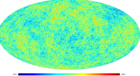
Figure 1: Sky map example synthesised using our MPI/CUDA implementation of thealm2maproutine. The
units areµK. An overall monopole term, with an amplitude of∼2.7 106µK, has been subtracted to uncover the minute fluctuations.
The specific goal of this work is to assist simulation and analysis efforts related to the Cosmic Microwave Background (CMB) studies. CMB is an electromagnetic radiation left over after the hot and dense initial phase of the evolution of the Universe, which is popularly referred to as the Big Bang. Its observations are one of the primary ways to study the Universe. The CMB photons reaching us from afar carry an image of the Universe at the time when it had just a few percent of its current age of ∼13Gyears. This
image confirms that the early Universe was nearly homogeneous and only small, 1 part in 105, deviations
were present, as displayed in Fig 1. Those initiated the process of so-called structure formation, which eventually led to the Universe as we observe today. The studies of the statistical properties of these small deviations are one of the major pillars on which the present day cosmology is built. On the observational front the CMB anisotropies are targeted by an entire slew of operating and forthcoming experiments. These include a currently observing European satellite called Planck1, which follows in the footsteps of two very
successful American missions, COBE2and WMAP3, as well as a number of balloon-borne and ground-based
observatories. Owing to quickly evolving detector technology, the volumes of the data collected by these experiments have been increasing at the Moore’s law rate, reaching at the present the values on order of petabytes. These new data aiming at progressively more challenging science goals not only provide, or are expected to do so, images of the sky with an unprecedented resolution, but their scientific exploitation will require intensive, high precision, and voluminous simulations, which in turn will require highly efficient novel approaches to a calculation of SHTs. For instance, the current and forthcoming balloon-borne and ground-based experiments will produce maps of the sky containing as many as O(105−106) pixels and
up toO(106−107)harmonic modes. Maps from already operating Planck satellite will consist of between 1
planck:http://sci.esa.int/science-e/www/area/index.cfm? fareaid =17
2
cobe:http://lambda.gsfc.nasa.gov/product/cobe/
3
O(106)andO(108)pixels and harmonic modes. The production of high precision simulations reproducing reliably polarized properties of the CMB signal, in particular generated due to the so called gravitational lensing, requires an effective number of pixels and harmonic modes, as big asO(109). These latter effects constitute some of the most exciting new lines of research in the CMB area. The SHT implementation, which could successfully address all this needs would not only have to scale well in the range of interest, but also be sufficiently quick to be used as part of massive Monte Carlo simulations or extensive sampling solvers, which are both important steps of the scientific exploitation of the CMB data.
At this time there are a few software packages available, which permit calculations of the SHT. These include,healpix[3],glesp[2],ccsht[1],libpsht[4], ands2hat[5], which are commonly used in the CMB research, and some others such as,spharmonickit/s2kit[6] andspherpack[7]. They propose different levels of parallelism and optimization, while implementing, with an exception of two last ones, essentially the same algorithm. Among those the libpshtpackage [23] offers typically the best performance, due to efficient code optimizations, and is considered as the state of the art implementation on serial and shared-memory platforms, at least for some of the popular sky pixelizations. Conversely, the implementation offered by thes2hatlibrary is best adapted to the distributed memory machines, and fully parallelized and scalable with respect to both memory usage and calculation time. Moreover, it provides a convenient and flexible framework straightforwardly extensible to allow for multiple parallelization levels based on hybrid programming models. Given the specific applications considered in this work, the distributed memory parallelism seems inevitable and this is therefore thes2hatpackage, which we select as a starting point for this work.
The basic algorithm we use hereafter, and which is implemented in both libpsht and s2hat libraries as described in the next section, scales as O(RN`2max), where RN is the number of rings in the analyzed map and`maxfixes the resolution and thus determines the number of modes in the harmonic domain, equal to '`2max. For full sky maps, we have usually `
max ∝ RN ∝n 1/2
pix, wherenpix is the total number of sky pixels, and therefore the typical complexity is O(`3
max) ∝ O(n 3/2
pix). We note that further improvements of this overall scaling are possible, for instance, if multiple identical transforms have to, or can, be done simultaneously, what could lower the numerical cost to essentially that of a single transform. In this paper we however focus on the core algorithm and leave an investigation of these potential extensions to future work.
We note that alternative algorithms have been also proposed, some of which display superior complexity. In particular, Driscoll and Healy [10] proposed a divide-and-conquer algorithm with a theoretical scaling of
O(npix ln2npix). This approach is limited to special equidistant sphere grids and being inherently numeri-cally unstable requires corrective measures to ensure high precision results. This in turn affects its overall performance. For instance, the softwarespharmonickit/s2kit, which is the most widely used implemen-tation of this approach, has been found a factor 3 slower than the healpix transforms implementing the standard O(n3/2pix)method at the intermediate resolution of`max∼1024[34]. Other algorithms also exist and typically involve a precomputation step of the same complexity, but often less favorable prefactors, as the standard approach, and an actual calculation of the transforms, which typically exploits either the Fast Multipole Methods, e.g., [28, 32] or matrix compression techniques, e.g., [18, 33], to bring down its overall scaling to O(npixlnnpix) [28], O(npixln2npix) [32, 33], orO(n
5/4
pixlnnpix) [18]. The methods of this class typically require significant memory resources needed to store the precomputation products and are advan-tageous only if a sufficient number of successive transforms of the same type has to be performed in order to compensate for the precomputation costs. The most recent, and arguably satisfactory, implementation of such ideas is a package calledwavemoth4 [25], which achieves a speed-up of the inverse SHT with respect to thelibpsht library by a factor ranging from3 to6 for`max ∼4000. In such a case the required extra memory is on order of40GBytes and it depends strongly, i.e.,∝`3max, on the resolution. We also note that
in some applications the need to use SHTs can be sometimes by-passed by resorting to approximate but numerically efficient means such as the Fast Fourier Transforms as for instance in the context of convolutions on the sphere as discussed in [11].
In many practical applications, as the ones driving this research, SHTs are just one of many processing steps, which need to be performed to accomplish a final task. In such a context, these are the memory high-water mark and algorithm scalability, which frequently emerge as the two most relevant requirements, as the cost of the SHT transforms is often subdominant and their complexity more favorable than that of many other typical operations. From the memory point of view, the standard algorithm, having the smallest memory footprint, remains therefore an attractive option. The important question is then whether its efficient, scalable, parallel implementation is indeed possible. Such a question is particularly pertinent
4
in the context of the heterogeneous architectures and hybrid programming models and this is the context investigated in this work.
The past work on the parallelization of SHTs includes a parallel version of the two step algorithm of Driscoll and Healy introduced by [16], the algorithm of [9] based on rephrasing the transforms as matrix operations and therefore making them effectively vectorizable, and a shared memory implementation avail-able in thelibpshtpackage. More recently, algorithms have been developed for NVIDIA General-Purpose Graphics Processing Units (GPGPU) [26, 15]. This latter work provided a direct motivation for the in-vestigation presented here, which describes what, to the best of our knowledge, is the first hybrid design of parallel SHT algorithms suitable for a cluster of GPU-based architectures and current high-performance multi-core processors, and involving hybrid OpenMP/MPI and MPI/CUDA programming. We find that once carefully optimized and implemented, the algorithm displays nearly perfect scaling in both cases, at least up to 128 MPI processes mapped on the same number of pairs of multi-core CPU-GPU. We find that inverse SHT with GeForce 400 Series equipped with the latest CUDA device ("Fermi") outperforms state of the art implementation for a multi-core processors executed on latest Intel Core i7-2600K, while the direct transforms in both these cases perform comparably.
This paper is organised as follows. In section 2 we introduce the algebraic background of the spherical harmonic transforms. In section 3 we describe a basic, sequential algorithm and list useful assumptions concerning a sphere pixelisation, which facilitate a number of acceleration techniques used in our approach. In following section, we introduce a detailed description of our parallel algorithms along with two variants suitable for clusters of GPUs and clusters of multi-cores. Section 5 presents results for both implementation and finally section 6 concludes the paper.
2
Algebraic background
2.1
Definitions and notations
Just as the Fourier basis facilitates a quick and efficient evaluation of convolutions in one or more dimensional spaces, the spherical harmonic basis does so but for functions defined on the surface of a sphere, i.e., depending on spherical coordinates: θ ∈ (0, π) (colatitude) and φ ∈ [0,2π) (the angle counterclockwise
about positivez-axis from the positivex-axis). We can express a band-limited approximationf˜to a
real-valued spherical functionf(θ, φ)f :S2→Rin terms of the spherical harmonic basis functions as
˜ f(θ, φ) = `max X `=0 ` X m=−` a`mY`m(θ, φ), (1)
where a`m are spherical harmonic coefficients describing f in the harmonic domain, Y`m is a spherical harmonic basis function of degree` and order m, and the bar over f indicates that it is merely a
band-limited approximation of f with a bandwidth `max. The spherical harmonic coefficients are computed by
taking the scalar inner product off with the corresponding basis function, which can be expressed as the
integral alm= π Z θ=0 2π Z φ=0 dθ dφ f(θ, φ)Ylm† (θ, φ) sinθ, (2)
where†denotes complex conjugation.
In actual applications the spherical harmonic transforms are rather used to project grid point data
(a discretized scalar field sn) on the sphere onto the spectral modes in an analysis step (as displayed in
equation (3)) and an inverse transform reconstructing the grid point data from the spectral information in asynthesis step (as displayed in equation (4)). Depending on the choice of`max and the grid geometry the transformsn →alm may only be approximate, what is indicated by a tilde over a.
˜ a`m = X {θn,φn} sn(θn,φn)Y`m(θn,φn), (3) sn(θn,φn) = `max X `=0 ` X m=−` a`mY`m(θn,φn). (4)
In CMB applications, sn is a vector of pixelized data, e.g. the brightness of incoming CMB photons, assigned tonpixlocations(θn, φn)on the sky defined as centres of suitable chosen sky pixels. The parameter
`maxdefines a maximum order of the Legendre function and thus a band-limit of the fieldsn, and in practice it is set by the experimental resolution.
The basis functions Y`m(θn,φn)are defined in terms of normalised associated Legendre functionsP`m of degreel and orderm,
Y`m(θn,φn)≡ P`m(cosθn)eimφn, (5)
where we use the relationYl,−m= (−1)mYlm† to compute all spherical harmonics in terms of the associated Legendre functions Plm with m ≥ 0. Consequently, by separating variables following equation (5) we can reduce the computation of the spherical harmonic transform to a regular Fourier transform in the longitudinal coordinateφn followed by a projection onto the associated Legendre functions,
˜ a`m = X {θn} X {φn} sn(θn,φn)eimφn P`m(cosθn) . (6)
The associated Legendre functions satisfy the following recurrence (with respect to the multipole number
`for a fixed value ofm) critical for the algorithms developed in this paper,
P`+2,m(x) =β`+2,mxP`+1,m(x) + β`+2,m β`+1,m P`m(x), (7) where β`m= r 4`2−1 `2−m2. (8)
The recurrence is initialised by the starting values,
Pmm(x) = 1 2mm! r (2m+ 1)! 4π 1−x 2m ≡ µm 1−x2 m , (9) Pm+1,m(x) = β`+1,mxPmm(x). (10)
The recurrence is numerically stable but a special care has to be taken to avoid under- or overflow for large values of`max [13] e.g., for increasing m thePmm values can become extremely small such that they can no longer be represented by the binary floating-point numbers in IEEE 7545 standard. However, since we
have freedom to rescale all the values ofP`m, we can dynamically rescale current values, while performing
the recurrence, to prevent a potential overflow on a subsequent step. More precisely on each step the newly computed value of the associated Legendre function is tested and rescaled if found to be too close to the over- or underflow limits. The rescaling coefficients (e.g., in form of their logarithms) are kept track of and used to rescale back all the computed values ofP`m at the end as required. This scheme is based on two facts. First, the values of the associated Legendre functions calculated via the recurrence change gradually and rather slowly on each step. Second, their actual values as needed by the transforms are representable within the range of the double precision values.
The specific implementation of these ideas used in all our algorithms follows that of thes2hatsoftware and the HEALPix package. It is based on a use of a precomputed vector of values, sampling the dynamic range of the representable double precision numbers and thus avoids any explicit computation of numerically-expensive logarithms and exponentials. This scaling vector is used to compare the values ofP`mcomputed on each step of the recurrence, and then it is use to rescale them if needed. For sake of simplicity, in this paper we assume that this is an integral part of associated Legendre function evaluation (independent of architecture) and we omit explicit description of algorithm related to rescaling. For more details we refer to [15] and documentation of the HEALPix package.
2.2
Specialized formulation
For a general grid of O(npix) points on the sphere, a direct calculation has computational complexity
O(`2
maxnpix)which is a serious limitation for problems in range of our interest. For instance, the current and forthcoming balloon-borne and ground-based experiments will produce maps of sky containing as many as npix ∈[105,106] pixels and up toO(106−107)harmonic modes. Maps from already operating Planck satellite will consist of betweenO(106)andO(108)pixels and harmonic modes. However, the algorithm we
use hereafter and which is described in the next section, scales asO(npix`max). We obtain such complexity with help of additional geometrical constraints imposed on the permissible pixelizations. These are [13],
5The IEEE has standardised the computer representation for binary floating-point numbers in IEEE 754. This standard is
• the map pixels are arranged on RN ≈
√
npix iso-latitudinal rings, where latitude of each ring is identified by a unique polar angleθn(for sake of simplicity hereafter we will refer to this angle by the ring index i.e.,rn→θn, wheren∈[0,RN])
• within each ring rn, pixels must be equidistant (∆φ=const), though their number can vary from a
ring to another ring.
The requirement of the iso-latitude distribution for all pixels helps to save on the number of required FLOPs as the associated Legendre function need now be calculated only once for each pixel ring. Conse-quently, nearly all spherical grids, which are currently used in CMB analysis (for instance HEALPix and GLESP), as well as other fields conform with such assumptions.
Taking into account these restrictions and definition of basis function Y`m (5) we can rewrite (adapted from [13]) the synthesis step from equation (4) as
s(rn,φn) = `max X m=−`max eimφ0∆A m(rn), (11) where∆A
m(rn)is a set of functions such as
∆Am(rn)≡ `max X `=0 a`0P`0(cosrn), m= 0, `max X `=m a`mP`m(cosrn), m >0, `max X `=|m| a†`|m|P`|m|(cosrn), m <0, (12)
and respectively the analysis step(3) as ˜ a`m= RN X n=0 ∆Sm(rn)P`m(cosrn), (13) where ∆Sm(rn)≡ X {φn} s(rn,φn)e−imφ0. (14)
Theφ0 denotes theφangle of the first pixel in the ring.
From above, we can see that the spectral harmonic transforms can be split into two successive computa-tions: one calculating the associated Legendre functions, Eqs. (12) and (13), and the other performing the series of Fast Fourier Transforms (FFTs), Eqs. (11) and (14) [20]. This splitting immensely facilitates imple-mentation, for instance, in order to evaluate Fourier transforms we can use third-party libraries devoted to this problem. However, we have to bear in mind that different libraries offer different robustness with strong dependence on length of FFT. This focus our special attention since the number of samples (pixels) per ring may vary and this strongly affects efficiency of the FFT algorithms. For instance, well-knowfftpack
library [29] used in healpix [13] andlibpsht [23] libraries performs well only for a lengthNF F T, whose prime decomposition only contains the factors2, 3, and5, while for prime number lengths its complexity
degrades fromO(NF F T logNF F T)toO(NF F T2 ). For this reason we employ by default in all versions of our algorithm theFFTWlibrary [12] which usesO(NF F TlogNF F T)algorithms even for prime sizes.
2.3
Time consumption
Three parameters typically determine the sizes and numerical complexity characteristic of our problem. These are a total number of pixels, npix, a number of rings of pixels in the analyzed map, RN, and a maximum order of the associated Legendre functions, `max. In particular a number of modes in the
harmonic domain is∼`2max. In well defined cases these three parameters are not completely independent. For example, in the case of full sky maps, we have usually`max∝ RN ∝n
1/2
pix. This imply that recurrence step requiresO RN`2max
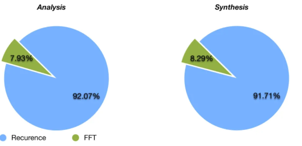
floating point operations (FLOPS), due to the fact that for each ofRN rings we have to calculate a full set, up to `max, of the associated Legendre functions, P`m, at cost ∝ `2max. The Fourier transform step, as mentioned above, has then subdominant complexityO(RN`maxlog`max). These theoretical expectations agree with our experimental results shown in Fig. 2 depicting a typical breakdown of the average overall time between the main steps involved in the SHTs computation as obtained for a run performed on quad-core Intel i7-2600K processor. We can observe that indeed the evaluation of the
Figure 2: The overall time breakdown between the main steps of the SHTs algorithm as computed with the identical band limit (`max= 4096) for quad-core Intel i7-2600K processor.
Legendre transform dominates by far over FFT in terms of time of computation. This motivated us to study the possible improvements of this part of the calculation. We explore this issue in the context of the heterogeneous architectures and hybrid programming models. In particular we introduce a parallel algorithm that is suitable for clusters of accelerators, namely multi-core processors and GPUs which we employ for an efficient evaluation of spherical harmonic transforms.
3
Basic algorithm
We proceed by developing algorithms which agree with assumptions listed in the previous section. Then, in the next section we introduce their parallel versions and we discuss possible improvements specific to the targeted architectures.
Algorithm 1 presents the computation of discrete, direct SHT which is a realisation of equation (3) for a given "bandwidth"`maxand input data vectorsobtained from the samples of the original function which we wish to transform. Respectively, algorithm 2 presents the computation of discrete, inverse transform
Algorithm 1Direct transform (Eq. 3)
Require: s∈Rnpix values step 1 -∆Sm(r) calculation
forevery ringrdo
foreverym= 0, ..., mmaxdo
◦calculate∆S
m(r)via FFT Eq.(14)
end for(m)
end for(r)
step 2 - Pre-computation foreverym= 0, ..., mmaxdo
◦µmpre-computation Eq.(9)
end for(m)
step 3 - Core calculation forevery ringrdo
foreverym= 0, ..., mmaxdo
forevery`=m, ..., `maxdo
◦computeP`mvia Eq.(7)
◦updatea`m, Eq.(13)
end for(`)
end for(m)
end for(r)
return a`m∈C`×m
from equation (3) which takes as input a set of complex numbersa`m, interpreted as Fourier coefficients in
Algorithm 2Inverse Transform (Eq. 4)
Require: a`m∈C`×mvalues
step 1 - Pre-computation foreverym= 1, ..., mmaxdo
◦µmprecomputation Eq.(9)
end for(m)
step 2 -∆Am calculation
forevery ringrdo
foreverym= 0, ..., mmaxdo
forevery`=m, ..., `maxdo
◦computeP`mvia Eq.(7)
◦update∆A m(r), Eq.(14) end for(`) end for(m) end for(r) step 3 -s calculation forevery ringrdo
foreverym= 0, ..., mmaxdo
◦calculatesvia FFT and given∆A
m(r), Eq.(11)
end for(m)
end for(r)
return s∈Rnpix
3.1
Similarities
Both algorithms use a divide and conquer approach i.e., in this approach our problem of computing projec-tion onto associated Legendre funcprojec-tions is decomposed into smaller subproblems of a similar form (rings of pixels). The subproblems are solved recursively by a further subdivision (computation ofP`mvia recurrence with respect to the multipole number` for a fixed value ofm) and finally their solutions are combined to
solve the original problem. Furthermore, both algorithms consist of three main steps:
• the pre-computation of the starting values of the recurrence (9) in the loop over all m ∈ [0, mmax] (step 2 in Algorithm 1 and step 1 in Algorithm 2 ),
• the evaluation of the associated Legendre function for each ring of pixels via the recurrence from equation (7). This requires three nested loops, where the loop over`is set innermost to facilitate the
evaluation of the recurrence with respect to the multipole number` for a fixed value ofm(step 3 in
Algorithm 1 and step 2 in Algorithm 2 ).
• step where via FFTs we either generate the cosine transform representation of the input vectors(11)
(step 1 in Algorithm 1) or to complete computation in inverse algorithm an abelian FFT is performed to compute the sums (14) (step 3 in Algorithm 2).
3.2
Differences
Both algorithms are almost the same in terms of number and type of arithmetic operations required for the computation (see for instance Figure 2 or a detailed analysis in [17]). The main difference consists in the dimension of the partial results which need to be updated within the nested loop where we evaluate the associated Legendre functions (step 3 in Algorithm 1 and step 2 in Algorithm 2). In case of the direct transform, for each ring of pixels on the sphere we need to update all non-zero values of the matrix
a`m∈C`max×mmax by a product between the precomputed inner sums defined as∆Sm (14) and associated Legendre function for each fixedm. In the case of the inverse transform, where the input is a set of complex
numbers a`m, the nested loop (step 2 in Algorithm 2) is used to compute the inner sum∆A
m (12), which can be obtained as a matrix-vector product
∆Am= ∆A m(r0, m) ∆Am(r1, m) ... ∆Am(RN, m) =
Pmm(cosr0) . . . P`maxm(cosr0)
Pmm(cosr1) . . . P`maxm(cosr1)
... ... ...
Pmm(cosrRN) . . . P`maxm(cosrRN) amm am+1m ... a`maxm . (15)
As we will see further in this report, those differences may cause big contrast in terms of evaluation time and memory consumption. This effect can be additionally enhanced by the type of the architecture on which we execute our algorithm.
4
Parallel Spherical Harmonic Transforms
4.1
Top-level distributed-memory parallel framework
The top level parallelism employed in this work is adopted from the S2HAT library developed by the last author. Though not new, it has not been described in detail in the literature yet and we present below its first detailed description including its performance model and analysis. The framework is based on a distributed-memory programming model and involves two computational stages separated by a single instance of a global communication involving all the processes performing the calculations. These together with a specialized, but flexible data distribution, are the major hallmarks of the framework. The two stages of the computations can be further parallelized and/or optimized and we discuss two examples of potential intra-node parallelization approaches below. We note that the framework as such does not imply what algorithm should be used by the MPI processes, e.g., [25], though of course its overall performance and scalability will depend on a specific choice.
The major motivation behind such a distributed memory parallelization level comes from the volumes of the data, both maps and harmonic coefficients, to be analyzed in the applications targeted here and from the need to maintain flexibility of the routines designed to be used in massively parallel applications, where SHTs typically constitute only one step of the overall process. The latter requirement calls not only for a flexible interface and an ability to use efficiently as many MPI processes as available, but also for a low memory footprint per process.
4.1.1 Data distribution and algorithm
The simple structure of the top-level parallelism outlined above is facilitated by a data layout, which assumes that both the mapsand its harmonic coefficientsa`m, are distributed. The map distribution is ring-based,
i.e., we assign to each process a part of the full map consisting of complete rings of pixels. To do so we make use of the assumed equatorial symmetry of the pixelization schemes and first divide all rings of one of the hemispheres (including the equatorial ring if present) into disjoint subsets made of complete, consecutive rings, and then assign to each process part of the map corresponding to one of such ring subsets together with its symmetric, counterpart from the other hemisphere. If we denote the rings mapped on a processori
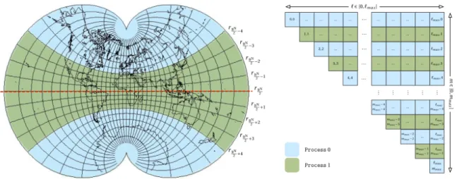
asRi, then∪nprocsi=0 Ri =R, whereRis the set of all rings andnprocsis the number of processes used in the computation. We also haveRi∩ Rj =∅ifi6=j. An example ring distribution is depicted in Figure 3(a), where different colours mark pixels on iso-latitudinal rings mapped on two different processes.
In order to distribute harmonic domain object we divide the 2-dimensional array of the coefficientsa`m with respect to a number,m, and assign to each process a subset of values ofm, Mi, and a corresponding
subset of the hamonic coefficients,{a`m:m∈ Mi and`∈[m, `max]}. As with the ring subsets, the subsets of m values have to be disjoint, Mi∩ Mj =∅ if i 6=j and include all the values, ∪
nprocs
i=0 Mi =M. An example of the harmonic domain distribution is depicted in Figure 3(b), where like in the case of the ring distribution we marked with different coloursa`mcoefficients mapped on two different processes.
This data layout allows to avoid any redundancy in terms of calculations and memory and any need for an intermediate inter-process communication, while at the same time is general enough that at least in principle can accommodate an entire slew of possibilities as driven by real applications. Any freedom in selecting a specific layout should be used to ensure a proper load balancing in terms of both memory and work, and it may, and in general will, depend on what algorithm is used by each of the MPI processes. Though perfect load balancing, memory- and work-wise, may not be always possible, in practice we have found that good compromises usually exist. In particular, the map distribution which assigns the same number of rings to each process is typically satisfactory, even if it may in principle lead to an unbalanced work and/or memory distribution. The latter is indeed the case for the healpixpixelization which does not preserve the same number of samples per ring, what introduces differences in the memory usage between the processes but also in the workload. Some fine tuning could be used here to improve on both these aspects, as it is indeed done ins2hat, but even without that the differences are not critical. For the distribution of the harmonic objects we propose Mi ≡ {m:m=i+k nprocs orm=mmax−i−k nprocs, wherek∈[0, mmax/2]}, so the process i stores the values of m equal to [i, i+nprocs, ..., mmax−i−nprocs, mmax−i]. This usually provides a good first try, which appears satisfactory in a number of cases as it will be explained in the next section.
(a) The iso-latitudinal rings distribution. (b) Distribution ofa`mcoefficients.
Figure 3: Example of a distribution of the iso-latitudinal rings and thea`mcoefficients among two processes. Each colour marks elements assigned to one process. For rings visualisation we used an August’s Conformal Projection of the sphere on a two-cusped epicycloid.
We note that this data layout imposes an upper limit on the number of processes which could be used, and which is given bymin(mmax/2,RN/2). This is typically sufficiently generous not to lead to any problems, as usually we haveRN ∝mmax'`maxand the limit on a number of processes isO(`max).
With this data distribution, Algorithms 1 and 2 require only straightforward and minor modifications to become functional parallel codes. As an example, Algorithm 3 details the parallel inverse transform, which is a parallel version of Algorithm 2. The operations listed there are to be performed by each of the
Algorithm 3General parallel alm2mapalgorithm ( Code executed by each MPI process )
Require: a`m∈C`×m form∈ Mi and all`
Require: indices of ringsr∈ Ri step 1 - Pre-computation
foreverym∈ Mi do
◦µmpre-computation Eq. (9)
end for(m)
step 2 -∆Am calculation
for every ringr∈ Randevery m∈ Mi do
◦initialise the recurrence: Pmm,Pm+1,m using precomputedµmEqs. (9) & (10)
◦precompute recurrence coefficients,β`mEq. (8)
for every`=m+ 2, ..., `max do
◦computeP`mvia the 2-point recurrence, given precomputedβ`m, Eq. (7)
◦update∆A
m(r), Eq. (12)
end for(`)
end for(r)and (m)
global communication ◦ ∆Am(r), m∈ Mi, allr∈ R MPI_Alltoallv⇐⇒ ∆Am(r), r∈ Ri, allm∈ M step 3 -sn calculation
forevery ringr∈ Ri do
◦via FFT calculates(r, φ)for all samplesφof ringr, given pre-computed∆A
m(r)for allm.
end for(r)
return sn for all(r∈ Ri)
nproc MPI processes involved in the computation. Like its serial counterpart, the parallel algorithm can be also split into steps. First, we precompute the starting values of the Legendre recurrenceµm (9), but only results form∈ Mi are preserved in memory. In next step, we calculate the functions ∆Amusing Eq. (12) forevery ring r of the sphere, but only form values in Mi. Once this is done, a global (with respect to
the number of processes involved in the computation) data exchange is performed so that at the end each process has in its memory the values of∆A
m(r)computed only for ringsr∈ Ribut forallmvalues. Finally, via FFT we synthesize partial results as in equation (11). From the point of view of the framework, steps 1 and 2 constitute the first stage of the computation, followed by the global communication, and the second computation involving here a calculation of the FFT. As mentioned earlier, though the communication is an inherent part of the framework, the two computation stages can be adapted as needed. Hereafter, we adhere to the standard SHT algorithm as used in Algorithm 3 .
4.1.2 Performance analysis
Operation count. We note that the scalability of all the major data products can be assured by adopting
an appropriate distribution of the harmonic coefficients and the map. This stems from the fact that apart of the input and output objects, i.e., maps and harmonic coefficients themselves, the volumes of which are inversely proportional to a number of the MPI processes by the construction, the largest data objects derived as intermediate products, are arrays ∆A or ∆S. Their sizes are in turn given as O(RNmmax/nproc), and again decrease inversely proportionally withnprocs. These objects are computed during the first computation
stage, subsequently redistributed as the result of the global communication, and used as an input for the second stage of the computation. Their total volume, as integrated over the number of processes, therefore also determines the total volume of the communication, as discussed in the next Section. As these three objects are indeed the biggest memory consumers in the routines the overall memory usage scales as
(npix+ 2mmax`max+RNmmax)/nprocs. For typical pixelization schemes, full sky maps, analyzed at its sampling limit, we havenpix∼`2max,`max'mmax, andRN ∼n
1/2
pix, and therefore each of these three data objects contribute nearly evenly to the total memory budget of the routines. Consequently, the actual high memory water mark is typically∼50% higher than the volume of the input and output data. We note that
if all three parameters,`max, mmax,RN, are allowed to assume arbitrary values memory re-using and, in particular, in-place implementations are not straightforward, as it may not be easy or possible to fit any of these data objects in the space assigned for others. For this reason, this kind of options are not implemented in the software discussed here.
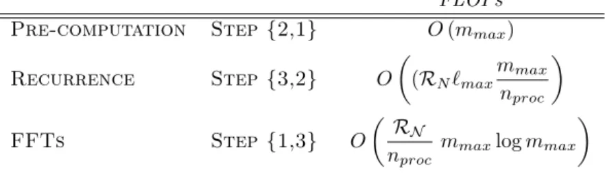
Given the assumed data layout, also the number of floating point operations (FLOPS) required for the evaluation of FFTs and associated Legendre functions scales inversely proportionally to the number of the processes. The only exception is related to the cost of the initialization of the recurrence (Eq. 9), which is performed redundantly by each MPI process to avoid an extra communication. Consequently, each process receives at least onemvalue on order ofmmax and has to perform at leastO(mmax)operations as part of the pre-computation, equation (9). A summary of the FLOPs required in each step of the parallel SHTs algorithms is presented in Table 1, where we have assumed here that the subsetsRi andMicontain
' RN/nproc and'mmax/nproc elements, respectively.
FLOPs
Pre-computation Step {2,1} O(mmax) Recurrence Step {3,2} O (RN`max mmax nproc FFTs Step {1,3} O RN nproc
mmaxlogmmax
Table 1: Number of floating point operations required in the parallel SHTs algorithm.
Communication cost. In order to determine the overall performance of the framework we have to also
estimate the communication cost. The data exchange is performed with help of a single collective operation of the type all-to-all in which each process sends data to, and receives from, every other process. We use a simple model to estimate the cost of the collective communication algorithms in terms of latency and bandwidth use i.e., we assume that the time taken to send a message between any two nodes can be modelled asα+β n, whereαis the latency (or startup time) per message, independent of message size,β
is the transfer time per byte, and n is the number of bytes transferred. However in case of the collective
communication routines, different MPI libraries use different algorithms, which moreover may depend on a size of the message. For specificity, we base our analysis on MPICH [19], a widely used MPI library. Similar considerations can be performed for other libraries.
The all-to-all communication in MPICH [31] for short messages (≤256kilobytes per message) uses the
index algorithm by Bruck et al. [8]. It is a store-and-forward algorithm that takes dlogne steps at the
expense of some extra data communication (β nlogninstead ofβ n). For long messages and even number
of processes, MPICH uses a pairwise-exchange algorithm, which takesnproc−1 steps. On each step, each process calculates its target process and exchanges data directly with that process i.e., data is directly communicated from source to destination, with no intermediate steps.
Note that in case of even distribution of rings r and m values, the size of message to be exchanged
between each pair of processes can be defined as
Smsg:=RN
mmax
nproc
nC, (16)
wherenCis the size in bytes of a complex number representation (usuallynC= 16).
Finally, merging all the assumptions listed above we can derive a following formula for the total time require for a communication in our parallel SHTs algorithm.
Tcomm = (
αlognproc+β Smsglognproc whenSmsg≤256 kB
α(nproc−1) +β Smsg (nproc−1) whenSmsg>256 kB
. (17)
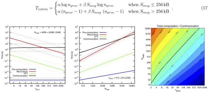
Figure 4: The two left most plots show theoretical run-times (logarithmic scale) as function of a number of processes and a fixed size of the problem, left most panel, and as a function of a resolution/size of the problem for the fixed number of processes, middle. The sizes of the problem shown in the leftmost panel with thick, solid lines, correspond to'2 108 pixels and corresponding harmonic modes, as given the HEALPix parameter valueNside= 4096. Thin, dashed lines show cases with4 times fewer (more) pixels, lower and upper lines respectively. In the middle panel the number of processes is assumed to benproc = 512, thick, solid line, or 256 (1024), as shown by thin dashed lines. The contours in the rightmost panel display a ratio of the total computation to communication times shown as a function of a number of process and size of the problem.
In Figure 4 we illustrate theoretical runtimes depending on the number of the employed processes (leftmost panel) and on the size of the problem (middle panel). The transform parameters have been set assuming a standard full sky, fully resolved case, and the HEALPix pixelization, i.e., `max = mmax =
2Nside, RN = 4Nside−1, npix = 12Nside. Here,2 Nside is the HEALPix resolution parameter (for more details see beginning of the section 5 and [13]). For the hardware parameters, in the estimation of the communication cost we have used following [24, 27]α= 10−5, β= 10−9, while for the cost of calculations we have assumed that each MPI process attains the effective performance of10Giga operations per second,
resulting in a time ofγ= 10−10seconds per FLOP. The choice we have made is meant to be only indicative, yet at its face value the latter number is more typical of the MPI processes being nodes of multi-cores than just single cores, in particular given the usual efficiency of such calculations, which is usually on order of 10−20%. If less efficient MPI processes are used then the solid curves in Fig. 4 corresponding to the
computation times should be shifted upwards by a relevant factor.
The dominant calculation is the recurrence needed to compute the associated Legendre functions in agreement with our earlier numerical result, Fig. 2. The computation scales nearly perfectly with the number of processed used decaying as∝1/nprocand it increases with growing size of the problem,∝Nside.2 At the same time the communication cost is seen to be independent on a number of processes. This is because for the considered here numbers of processes the size of the message exchanged between any two
processes is always large and the communication time is thus described by the second term of the second equation of Eqs. 17. Given that the single message size,Smsgs, decreases linearly with a number of processes,
the total communication time does not depend on it. The immediate consequence of these two observations is that both these times will be found comparable if sufficiently large number of processes is used. A number of processes at which such a transition takes place will depend on the constants entering in the calculation of Eqs. 17 and the size of the problem. This dependence of the critical number of processes on the size of the problem is shown in the rightmost panel of Fig. 4 with thick solid contour labelled 1.0. Clearly,
from the perspective of the transform runtimes there is no extra gain, which could be obtained from using more processes than given by their critical value. In practice, a number of processes may need to be fixed by memory rather than computational efficiency considerations. As the memory consumption depends on the problem size, i.e., npix, in the same way as the communication volume, by increasing the number of
processes in unison with the size of the problem we can ensure that the transform runs efficiently, i.e., the fraction of the total execution time spent on communicating will not change, and that it will always fit within the machines memory.
We note that some improvement in the overall cost of the communication could be expected by employing a non-blocking communication pattern applied to smaller data objects, i.e., single rows of the arrays, ∆A and∆S corresponding to a single ring ormvalue, successively and immediately after they become available. Though such an approach could extend the parameter space in which the computation time is dominant and the overall scaling favorable, it will most likely have only a limited impact given that the same, large, total volume of the data, which needs to be communicated. The communication volume could be decreased, and thus again the parameter space with the computation dominance extended, if redundant data distributions and redundant calculations are allowed for in the spirit of the currently popularcommunication avoiding
algorithms, e.g., [14]. Though these kinds of approaches are clearly of interest they are outside of the scope of this work and are left here for future research.
We also not that the conclusions may disfavour algorithms which require on the one hand big memory overhead and/or need to communicate more. Such algorithms will tend to require a larger number of processes to be used for a given size of the problem and thus will quickly get into bad scaling regime. Their application domain may be therefore rather limited. We emphasize that this general conclusion should be reevaluated case-by-case for any specific algorithms. Likewise, it is clear that the regime of the scalability of the standard SHT algorithm could be extended by decreasing the communication volume. Given that the communicated objects are dense, the latter would typically require some lossy compression techniques, we do not consider them here. Instead we focus our attention on accelerating intra-node calculations. This could improve the transforms runtimes for a small number of processes, however, if successful unavoidably will also result in lowering the critical values for the processes numbers. leading to losing the scalability earlier. Nevertheless, the overall performance of these improved transforms would never be inferior to that of the standard ones whatever a number of processes.
4.2
Exploiting intra-node parallelism
In this Section we consider two extensions of the basic parallel algorithm, Algorithm 3, each going beyond its MPI-only paradigm. Our focus hereafter is therefore on the computational tasks as performed by each of the MPI processes within the top-level framework outlined earlier. Guided by the theoretical models from the previous Section we expect that any gain in performance of a single MPI process will translate directly into analogous gain in the overall performance of the transforms at least as long as the communication time is subdominant, i.e., in a relatively broad regime of cases of practical importance. Hereafter we therefore develop implementations suitable for multi-core processors and GPUs and discuss the benefits and trade-offs they imply.
As highlighted by Fig. 4, of the three computational steps, this is the recurrence used to compute the associated Legendre functions which takes by far the dominant fraction of the overall runtime. Consequently, we will pay special attention to accelerating this part of the algorithm, while we will keep on using standard libraries to compute the FFTs. The latter will be shown to deliver a sufficient performance given our goals here. The associated Legendre function recurrence involves three nested loops and we will particularly consider the benefits and downside of their different ordering in order to attain the best possible performance. Hereafter, for simplicity we will refer to the algorithms for direct and inverse spherical transforms by the core names of their corresponding routines i.e.,map2almandalm2maprespectively.
4.2.1 Multithreaded version for multi-core processors
Since the largest and fastest computers in the world today employ both shared and distributed memory architectures, software which use only a distributed memory approaches such as MPI may not fully exploit
the shared memory underlying architecture and thus may loose some efficiency. Shared memory approaches, based on explicit multithreading or language-generated multithreading (e.g. OpenMP) are more accurate on shared memory architectures. Thus, many hybrid approaches, typically mixing MPI and OpenMP, have been proposed to better exploit clusters of of multi-core processors. In this spirit, we introduce the second level of parallelism based on multithreaded approach in the computation of SHTs.
As discussed shortly at the beginning of this section, the order of the three nested loops can be changed. For instance, the iterations overm in the outermost loop allow precomputing β`m Eq. (8), Pmm Eq. (9) andPm+1,m Eq. (10) only once for each ring with extra storage of an orderO(`max). But in this case we also need to store intermediate products which require additional O(RN`max) storage comparable to the size of the input and output. However modern super computers are equipped with memory banks of size in tens of GB. This fostered us for developing multithreaded versions of Algorithm 1 and 2 in which we
place loop overm outermost. That is, we introduced the multithread layer via OpenMP for m loop i.e.,
a set of m∈ Mi values (already assigned to ith MPI process) is evenly divided into a number of subsets equal to the number of threads mapped onto each physical core available on a given multi-core processor. We denote this subset ofmvalues as MT
i where subindex iis an ith thread. In such a way each physical core executes one thread concurrently and calculates intermediate results of SHTs for its local (in respect to shared memory) subset ofm. The Algorithm 4 describes thestep 1of Algorithm 3 in its multithreaded
version.
Algorithm 4∆A
m calculation per thread
Require: allm∈ MT i ⇒ Nth S i=1 MT i =Mi forallm∈ MT i do ◦initialisePmm Eqs. (9)
for every ringrdo
for every `=m+ 2, ..., `max do
◦precomputeβ`mEq. (8)
◦computeP`mviaβ`m, Eq. (7)
◦update∆A
m(r)in shared memory, Eq. (12)
end for(`)
end for(r)
end for(m)
Load balance between active threads
Selecting a loop overmas an outermost one is certainly the best approach from the point of view of speed
optimization (see previous subsection), but such configuration leads to poor load balance. Notice that due to assumptions listed in section 2.2 the`-recursion starts from `=m(see for example Eq. 12). Therefore,
the number of flops required for evaluating the recurrence from equation (9) differs for differentm. For that
reason, we have to carefully map subsetsMT
i onto active threads to ensure that the total time required for the evaluation of the problem on a given node will be equally divided by the number of available cores.
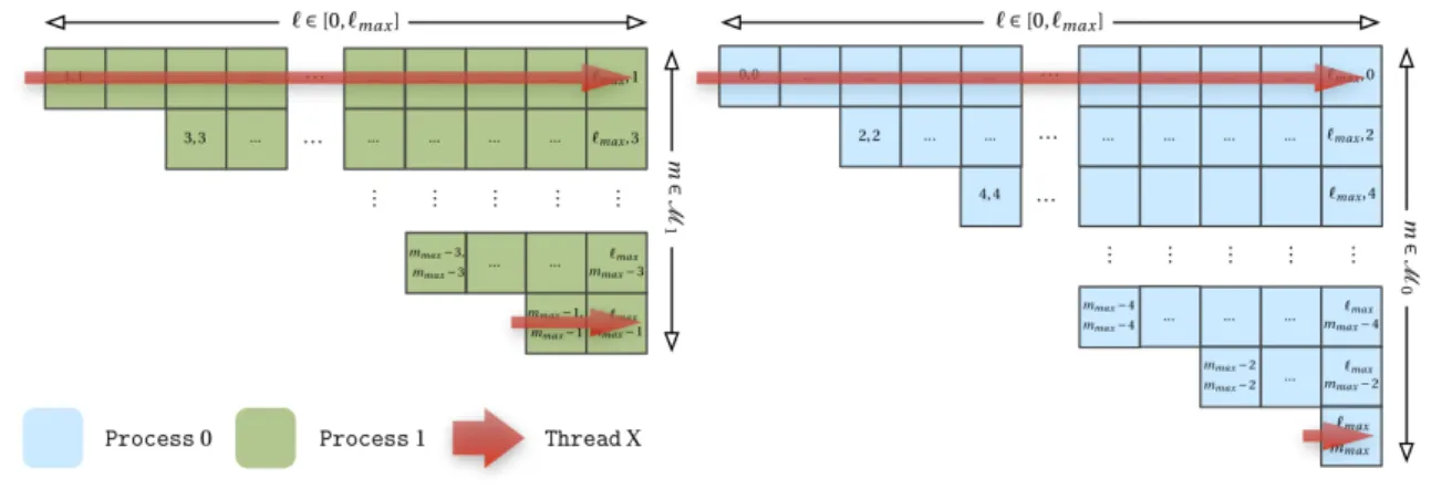
Because the lenght of the loop over ` decreases with growing number ofm, we create subsetsMT i by taking values from the setMi in "max-min" fashion i.e., iteratively we take fromMi the maximum value and the minimal one and we assign them to a chosen thread. In the same moment we try to equilibrate the number of such pairs within each subsetMT
i . Example of a such a mapping is depicted in Figure 5. In next subsection, we introduce a similar multithreaded approach for accelerating the projection of associated Legendre functions using GPU.
4.2.2 SHTs on GPGPU
A CUDA (Compute Unified Device Architecture) device is a chip consisting of hundreds of simple cores, called Streaming Processors (SP) which execute instructions sequentially. Groups of such processors are encapsulated in a Streaming Multiprocessor (SM) which executes instruction in a SIMD (Single Instruction, Multiple Data) fashion. Therefore each SM manages hundreds of active threads in a cyclic pipeline in order to hide memory latency i.e., a number of threads are grouped together and scheduled as a Warp, executing the same instructions in parallel. Therefore CUDA threads are grouped together into a series of thread blocks. All threads in the thread block execute on the same SM, and can synchronise and exchange data using very fast but small (up to 48KB in size for the latest NVIDIA carts) shared memory. The shared
Figure 5: Example of two "min-max" pairs of m values assigned to Thread X on Process 1 (left) and 0
(right) respectively. The read arrow represents the direction and the lenght of the`-recurrences (Eq. 10)
evaluated by a thread for a given "min-max" pair.
memory can be used as a user-managed cache enabling higher bandwidth than direct data copy from the slow device global memory.
The restrictions related to memory (both size and speed) and the lack of synchronisation between the blocks of threads drive the structure of our algorithms devised for GPUs. For instance, placing the loop over m as outermost (like in algorithms dedicated for multi-core CPUs) is not appropriate for CUDA
applications due to the memory size limitation. Consequently, the vectorβ`m cannot be entirely stored in shared memory. Its values would need to be recomputed for eachmand accessed sequentially in the`-loop.
A possible implementation would require re-computing theβ`mcoefficients for each pass through the`-loop, which would significantly affect the performance. Therefore, to agree with the philosophy of programming for GPUs, which consists in using fine grained parallelism and launching a very large number of threads in order to use all the available cores and hide memory latency, we set iterations overr in the outermost
loop and parallelize it in such a way that a number of rings (preferably only one) is assigned to one thread. In this model each thread computes the 2-point recurrence for all available m-values (but we assume that
GPU is a part of distributed memory system therefore) in contiguous fashion as depicted on Figure 6. This makes it straightforward to plan the computation ofβ`mvia Eq. (9) in batches, which can be cached and shared inside a thread block. Note that in case of distributed memory systems the number ofm values in
setMi may vary for different i, while the total number of ringsRN stays constant. Therefore, it is easier to plan good load balance for GPU when we parallize our algorithms overr loop.
Figure 6: Schematic view of `-recurrence iterations (eq. 10) evaluated by each thread on CUDA device
assigned to Process1 and0respectively.
Setting loop over rings outermost in our nested loop triggers two completely different approaches for memory management in direct and inverse SHTs. Therefore we dedicate the following two subsections to describe in detail the differences betweenmap2almandalm2mapalgorithms for GPUs.
map2alm
Mapping rings onto big number of threads, indeed facilitates the parallelization of SHTs algorithm on GPUs i.e., in such set-up each active thread perform exactly the same number and type of operations but with
different values. However, the direct transform requires that for each ring we update all non-zero values of the matrixa`,m∈Cmmax×`max. This leads to all-reduce operation6 between active threads. This is to say, the partial results generated by all active threads need to be summed together and written in the memory space from which we will read the final solution after all threads will be executed. Note that on CUDA, active threads can communicate only in thread block, which makes this task more difficult.
The Algorithm 5 outlines the Step 3 of algorithm 1 adapted to CUDA. We assume however that we are working on a memory distributed system, therefore the range ofm values is limited toMi. To ensure
workaround for the high latency device memory and take advantage of the fast shared memory, we first calculate the values of β`m vectors in segments, which allows us to fit them to the shared memory i.e., all threads within a block in a "collaborative" way compute in advance β`m values and store them in shared memory. Next, we use those precomputed values to evaluate associated Legendre functionP`m(r). After, each active thread fetches from global memory a precomputed sum ∆Sm(r) and performs a final multiplication Eq. (13). Once it’s done, we sum all those partial results within a given block of threads using adapted7version of parallel reduction primitive from CUDA SDK. For such locally reduced result one
thread in block updates corresponding entry in global memory. This implies thatj=NBT(number of blocks
of threads) threads will try to increase the value of a variable at the same space of global memory - which is referred to as arace condition problem, common in multithread applications. Fortunately, race conditions are
easy to avoid in CUDA by using atomic operations. An atomic operation is capable of reading, modifying, and writing a value back to memory without the interference of any other threads, which guarantees that a race condition will not occur. Therefore, all final updates of final results in global memory are performed via CUDAatomicAddfunction. In case when atomic functions are not supported on a given GPU we can
easily avoid race conditions by increasing granularity of recurrence step. In this scenario we loop over m
values on CPU and execute Mi "smaller" CUDA kernels which for a fixed values m and µm, evaluate
NBTreduced (per block of threads) resultsa?`m, which are next copy from device to host memory and sum together using CPU. This variant of our algorithm corresponds to the state HYBRID_EVALUATION = true,
in listing 5.
alm2map
The inverse SHT also requires the reduction of partial results, but in contrary to the direct transform, we need to sum them for all` as displayed in Eq. (12). With rings assigned to single threads, this leads to
rather straightforward implementation. Algorithm 6 outlines thealm2mapalgorithm devised for GPUs and
it is based on the version detailed in [15], which conforms with all assumptions stated in this paper. First, we partition the vector of thea`mcoefficients in the global memory into small tiles. In this way a block of threads can fetch resulting segments in sequence and fit them in the shared memory. Next, we calculateβ`mvalues in the same way as in the map2almalgorithm. With all the necessary data in the fast shared memory, in following steps, each thread evaluates in parallel an associated Legendre function and updates the partial result∆Am. In contrast to the direct transform, those updates are performed without a
race condition problem i.e., each thread stores its temporary values in small space of the shared memory to which it has an exclusive and very fast access. Once, the loop over all` is finished, the final partial result
is written to the global memory.
4.3
Exploitation of hybrid architectures
Many new supercomputers are hybrid clusters i.e., they are a combination of computational nodes intercon-nected (usually via PCI-Express bus) with multiply GPUs. In such a way, one or more multi-core processors have access to one GPU. Facing these heterogeneities, the front end user of the spherical harmonic package will have to decide which type of architecture to choose for calculation. The three-stage structure of our algorithms allows us to freely map different steps of the algorithms onto different accelerators in hybrid system. However, the steps have to be evaluated sequentially in unchanged order. The intention of this flexibility is to facilitate selection of the most efficient library for FFTs e.g. NVIDIA provides its own library for FFT on GPUs i.e.,CUFFT[21] which efficiency strongly depends on the version of CUDA device and the
version of the routine. Therefore, on some supercomputers with highly tuned version of FFTW3 library, FFTs perform better on multi-core CPUs. Note that our algorithms require the evaluation of FFTs on complex data, which length may vary from ring to ring.
In practice, on heterogeneous systems we assign each step of the algorithm to the architecture on which it performs faster. The default assignment for both transformation is depicted in Figure 7. Note that due
6Reduce-type operation combines the distributed elements using predefined operation (e.g., summation, multiplication etc.)
and returns the combined value in the output buffer.
Algorithm 5a`m calculation on CPU&GPU
Require: ∆S
m &µmvectors in GPU global memory form∈ Mi
for every ringrassign to one GPU threaddo foreverym∈ Mi do
for every `=m+ 2, ..., `max do
•use precomputed or, if needed, precompute in parallel a segment ofβ`m(8);
•computeP`mvia Eq. 7;
•evaluate: ar`m=∆mS (r)P`m(r)
•sum all partial resultsar`mwithin a block of threads
a?`m= NTPB X i=0 (ar`m)i (18) if HYBRID_EVALUATION then
• for each block of threads with different id =BID, writea?
`m in global device memory
aGP U`m [BID] =a?`m
• copy partial resultsaGP U
`m [. . .]from device to host memory and sum together using CPU
fori= 0→NBTdo a`m=a`m+aGPU`m[i]
end for else
• updatea`min global memory via atomic addition: a`m=a`m+a?`m
end if end for(`)
end for(m)
end for(r)
return a`,m∈Cmmax×`max
Algorithm 6∆A
m calculation on GPU
Require: a`,m∈Cmmax×`max matrix in GPU global memory
for every ringrassign to one GPU threaddo form∈ Mi do
for every `=m+ 2, ..., `max do
•use fetched or, if needed, fetch in parallel a segment ofa`m data;
•use precomputed or, if needed, precompute in parallel a segment ofβ`m(8);
•computeP`mvia Eq. 7;
•update∆Am(r)for a given prefetcheda`m and computedP`m(12);
end for(`)
•save final∆A
m(r)in global memory
end for(m)
end for(r)
return vector of partial results: ∆A m∈C
to their sequential nature, we omit steps in which we evaluate the starting values of the recurrence Eq. (9) (step 2 in Algorithm 1 and step 1 in Algorithm 2), which are always computed on CPU.
Figure 7: Default assignment of the major steps of the SHTs algorithm to one of the two architectures, multi-core processor or GPU, in a GPU/CPU heterogeneous system. Step 3 inmap2alm algorithm covers
two architectures due to optional use of CPU for reducing partial results between the execution of the CUDA kernels.
5
Numerical experiments
In order to evaluate the accuracy, efficiency and scalability of our new algorithm, we perform a series of tests with different geometry of the 2-sphere grid and different values of `max and mmax. To validate our algorithms, in each experiment we perform a pair of backward and forward SHTs starting out with a backward transform on a set of randomainit
`m coefficients which are uniformly distributed random numbers in the range(−1,1). To measure the accuracy of the algorithm we analyse the resulting map and we calculate
the error as the difference between the final outputaout
`m and the initial set a init
`m via the following formula,
Derr = v u u u u t P ` P m ainit`m −aout`m 2 P ` P m ainit`m 2 . (19)
The pairs of transforms were tested on HEALPix grids with a different resolution parameter Nside.
Accordingly to this parameter npix = 12Nside,2 RN = 4Nside −1 where maximum lenght of the ring (equator) is equal to 4Nside. Finally we also choose `max = mmax = 2×Nside, except for some specific experiments.
5.1
Validation against other implementation
In this experiment, a set of ainit
`m coefficients with a different value of `max was generated, then a pair of backward and forward transforms were performed to converted ainit
`m to a HEALPIx map with a fixed
Nside= 1024and then back to aout`m. Starting with the same input array we used our both implementation (MPI/OpenMP & MPI/CUDA) and thelibpshtlibrary [23] to evaluate transforms. We measured the total
time and the final errorDerr Eq. (19).
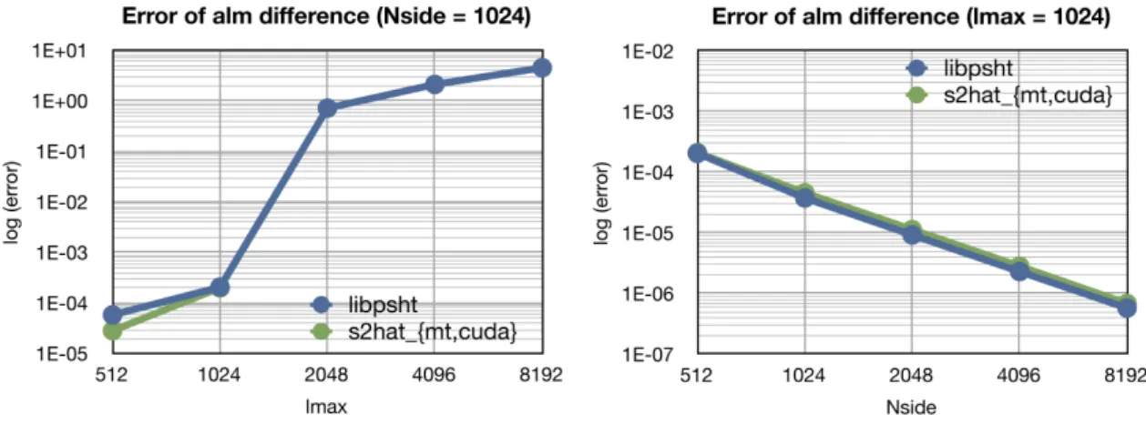
Figure 8 depicts Derr errors for s2hat_{mt,cuda} andlibpsht transforms pairs on HEALPIx grids with various`maxandNside values. Every data point is the maximum error value encountered in the pairs of transforms. As we can observe, all implementations provide almost identical quality of solutions with respect to different sizes of the problem.
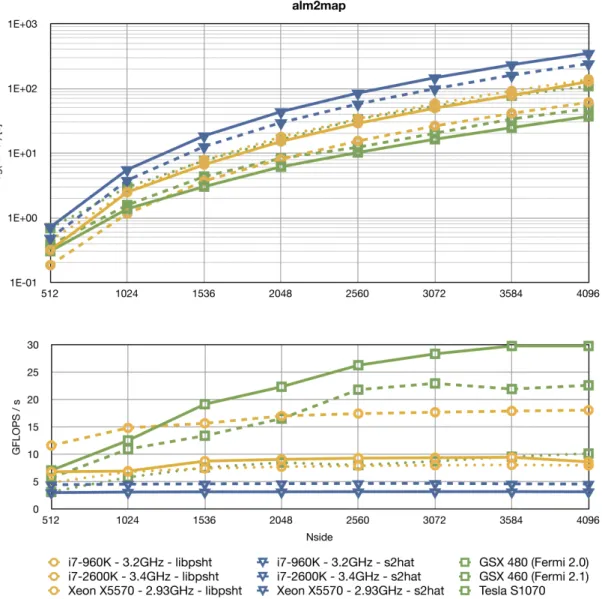
5.1.1 Scaling with growing resolution and performance comparison with libpsht
To study the time scaling of the algorithm with growing resolution of the problem defined via Nside pa-rameter, we perform a number of experiments with variousNside =`max/2 parameter. Like in previous experiment we compare our results withlibpsht package.
We choose Martin Reinecke’slibpshtbecause it is to our knowledge, the fastest implementation of SHTs
suitable for an astrophysical application and it is essentially a realisation of the same algorithm as the one used in our parallel algorithm. This highly optimized implementation is based on explicit multithreading and SIMD extensions (SSE and SSE2) but its functionality is limited to the shared memory systems only.
Figure 8: Derr fors2hat_{mt,cuda}andlibpshttransforms pairs on HEALPIx grids with various`max andNside. Every data point is the maximum error value encountered in transforms pairs. Loss of precision
seen in the left panel for`max∼>2048 and shared by both implementations is due to aliasing inherent to the adopted pixelization scheme.
CPU clock speed GPU Compilators line style
Core i7-960K 3.20 GHz GeForce GTX 480 gcc 4.4.3 / nvcc 4.0 solid line Core i7-2600K 3.40 GHz GeForce GTX 460 gcc 4.4.5 / nvcc 4.0 dashed line Xeon X5570 2.93 GHz Tesla S1070 icc 12.1.0 / nvcc 4.0 dot line Table 2: Different Intel multi-core processors and NVDIA GPUs used in our experiments.
Consequently, we perform all comparison experiments with only one pair of multi-core processor and GPU on three different systems listed in Table 2.
In a similar fashion as in our multithreaded version, all CPU-intensive parts of libpsht’s transforms
algorithm are instrumented for parallel execution on multi-core computers using OpenMP directives. There-fore, in all our tests we set-up for all runs a number of OpenMP threads equal to the number of physical
cores (OMP_NUM_THREADS= 4).
The range of pixelization sizes was limit by the size of the memory of a single GPU. Therefore we limit our tests toNside= 4096. We also limit timing measurement in this experiment to the recurrence part only (step 3 in Algorithm 1 and step 2 in Algorithm 2), however in case of CUDA routines, those measurements includes also the time spend on any data movements between GPU and CPU.
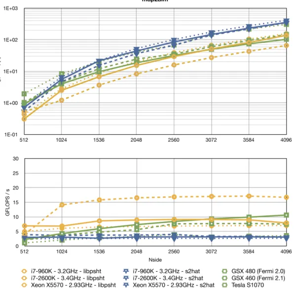
The results of this experiment are shown in Figures 9 and 10. The figures depict the measured times in seconds and the number of Gflops per second in logarithmic scale. The number or flops include all the operations necessary for the purpose of the numerical stability like rescaling in case ofs2hatroutines (see paragraph 2).
As expected, our multithreaded version is always slower in comparison tolibpshtby a constant factor.
Mainly, due to lack of SSE intrinsics in our code, which allows on some hardware to perform two or more arithmetic operations of the same kind with a single machine instruction. Especially on latest intel i7-2600K processor, SSE optimised libpsht implementation takes advantage of the extended width of the SIMD
register8 and Advanced Vector Extensions (AVX) which significantly increase parallelism and throughput
in floating point SIMD calculations.
The other important observation is that forward and backward SHTs on CPU, with identical param-eters, require almost identical time. Furthermore, performance analysis allows several deductions about performance of GPU version of SHTs algorithms.
• It is fairly evident that forward transform on CUDA with slower, not only with respect to its CPU version, but also in comparison with backward transform on the same architecture. Since the imple-mentation of the CUDA kernel for realisation of projection onto associated Legendre polynomials is essentially the same for both directions of the transform, the performance lost is mainly due to very
8The width of the SIMD register in file on i7-2600K is increased from 128 bits to 256 bits in respect with previous generation
Figure 9: Benchmarks for direct SHT performed on different (see Table 2 for details) pairs of Intel multi-core processor with GPU on a HEALPIx grid. The top plot shows timings for projection on Legendre polynomials, the libpsht code (orange circles) is compared with hybrids2hatcodes (blue&green lines). In each case we use a HEALPIx grid withNside=`max/2. In case of CUDA routines, timings include time of data movements between CPU and GPU. Bottom pane shows number of GFLOPS per second. Note that CUDA routines loose performance in comparison to the SSE optimised lipsht due to very costly reduction of partial results. First in shared memory and then on host memory with use of CPU. Nevertheless, NVIDIA GTX 480 outperforms libpsht on Core i7-960K.
Figure 10: Benchmarks for inverse SHT performed on different (see Table 2 for details) pairs of Intel multi-core processor with GPU on a HEALPIx grid. The top pane shows timings for projection on Legendre polynomials, the libpsht code (orange circles) is compared with hybrids2hatcodes (blue&green lines). In each case we use a HEALPIx grid withNside=`max/2. In case of CUDA routines, timings includes time of data movements between host and device. Bottom pane shows number of GFLOPS per second. Note that GeForce 400 Series equipped with latest CUDA architecture (codename "Fermi") outperform libpsht on the latest, Intel Core i7-2600K. Bear in mind that GeForce family is not design for professional use therefore their double-precision throughput has been reduced to 25% of the full design.