Large Eddy Simulation of Turbulent Incompressible Flow Using GPU with Multigrid Algorithm

(1)

Large Eddy Simulation of Turbulent Incompressible

Flow using GPU with multigrid algorithm

By

Mudassar Shaikh

Roll No. ME11M16

M.Tech II Yr.-Thermofluids

A Thesis Submitted

in Partial Fulfillment of the Requirements

for the Degree of

Master of Technology

Department Of Mechanical Engineering

Indian Institute Of Technology Hyderabad

(2)

(3)

(4)

Acknowledgements

I would like to thank my guide Dr Raja Banerjee for giving me an opportunity to work with him.His guidance in my research work has been invaluable. He has managed to be strict and patient at the same time, during the most demanding times of the work. He is a great person and one of the best mentors, I will always be thankful to him.

I would also like to thank Sathi Rajesh Reddy for his friendly support and encour-agement through the entire work of this dissertation. A special note of thanks to all my classmates from Thermal Engineering for inspiring me to do my best always. I would also like to thank all my juniors especially Vatsalya Sharma and Varun Jadon for being a greate support especially during culmination phase of this dissertation. I would also like to thank Mr Madhu Pandicheri for his timely support in the CAE lab. A special note of thanks to all my dear friends in the hostel especially my room mate Pankaj Kumar for making my stay in IIT Hyderabad memorable and enjoyable.

I would like to dedicate this thesis to my amazingly loving and supportive family who has always been with me, no matter where I am.

(5)

(6)

Abstract

The research presented in this dissertation is divided into two parts,the first part fo-cuses purely on computational science, and the second part fofo-cuses on fundamental fluid dynamics. The computational science aspect involves implementing an incom-pressible Navier-Stokes solver on Graphics Processing Units (GPUs), with optimized algorithm like multigrid algorithm to achieve the goal of enhancing performance of existing computational facilities and enabling them to solve more complex and com-putationally expensive fluid flow problems. The fluid dynamics aspect involves using the GPU-based Navier-Stokes solver to study turbulent flows. Large Eddy Simulation (LES) turbulence model has been implemented successfully to analyze 2d incompress-ible flow.

Computational Fluid Dynamics (CFD) simulations can be very computationally ex-pensive,especially for Large Eddy Simulations (LES). In LES the large, energy contain-ing eddies are resolved by the computational mesh, but the smaller (sub-grid) scales are modeled. Clusters of CPUs have been the standard approach for such simulations, but an emerging approach is the use of Graphics Processing Units (GPUs), which de-liver impressive computing performance compared to CPUs. Recently there has been great interest in the scientic computing community to use GPUs for general-purpose computation (such as the numerical solution of PDEs) rather than graphics render-ing. To explore the use of GPUs for CFD simulations, an incompressible Navier-Stokes solver was developed for a GPU. The Navier-Stokes equation is solved via a SMAC algorithm and is spatially discretized using the finite volume method on a rectangular collocated grid. Validation of the GPU-based solver was performed for fundamental bench-mark problems, and a performance assessment indicated that the solver was over an order-of-magnitude faster compared to a CPU. This solver was later extended to perform an LES of turbulent flows. LES has been known to be sensitive to inlet bound-ary conditions, the effect of different inlet boundbound-ary conditions has been observed and summarized for a mixing layer problem.

(7)

List of Figures

1.1 Heirarchy of Levels . . . 6

2.1 GPU Thread Hierarchy . . . 13

2.2 Memory model of GPU . . . 14

2.3 CUDA thread mapping arrangement . . . 15

2.4 V cycle for 3 levels . . . 16

3.1 2nd order UPWIND . . . 22

4.1 Energy spectrum for a turbulent flow . . . 32

5.1 Lid driven cavity Problem . . . 37

5.2 U v/s Y Red Black GS . . . 39

5.3 V v/s X Red Black GS . . . 39

5.4 U v/s Y Red Black GS on multigrid . . . 41

5.5 V v/s X Red Black GS on multigrid . . . 42

5.6 Mixing layer problem . . . 42

5.7 Steady state Mixing layer profile obtained . . . 43

5.8 Comparing mid plane velocity profile . . . 44

5.9 Inlet Profile for LES . . . 46

5.10 X-Velocity contour for Cs=0.17 . . . 48

(10)

List of Tables

1.1 Grid Size for DNS and LES . . . 4

5.1 Runtime GPU vs serial code . . . 38

5.2 Variation of workunits with levels . . . 40

5.3 Comparison GPU single vs Multigrid . . . 40

5.4 GPU vs serial comparison k- . . . 44

(11)

(12)

Chapter 1 Introduction

1.1 General Introduction

In recent years the power and diversity of flow simulations as a tool for exploring science and technology involving flow applications have reached new levels. This offers a promising future for providing cost effective alternatives to laboratory experiments, field tests and prototyping. This new power of flow simulation is based mainly on recent developments in high performance computing. Advanced algorithms capable of accurately simulating complex, real world problems and advanced hardware and networking with sufficient memory and bandwidth to execute those simulations are being developed. The flow simulation solvers have come a long way to a point of being a practical tool for solving complex real world problems in different fields of engineering and applied fluid mechanics.

In turbulence modeling RANS approach is useful for qualitative descriptions of flows. However it is unreliable for extracting detailed flow physics. RANS simulation gives a profile which is averaged over time and their solutions do not resolve the wide range of length and time scale that is typically seen in turbulent flows. In various engineering applications scientists or engineers are more interested in the description of large scale fluctuations of flow which contain the desired information of turbulent transfer of mo-mentum, heat and other scalars. This can be achieved by directly solving Navier Stokes equation at all scales as in Direct Numerical Simulations(DNS) or resolving large scale fluctuations as in Large Eddy Simulation (LES). However, DNS and LES are compu-tationally expensive.The computational requirement for LES & DNS is illustrated in Table 1.1.(Wilcox [16]) for a 3D channel flow. As can be seen from the table, there is

(13)

4 1.2 CFD using Graphics Processing Units ReH Reτ NDN S NLES 12300 360 6.7X106 6.1X105 30800 800 4X107 _3.0X106 616000 1450 1.5X108 _1X107 230000 4650 2.1X109 _1X108

Table 1.1: Grid Size for DNS and LES

rapid increase in computational cost with increase in Reynolds number. In such high fidelity computation, multicpu based High Performance computing cluster has been traditionally used.

1.2 CFD using Graphics Processing Units

Overview

Driven by the demands of the gaming industry, the graphics hardware has substan-tially evolved over the years with remarkable floating point arithmetic performance. Small-footprint desktop supercomputers with hundreds of cores that can deliver ter-aflops peak performance at the price of conventional workstations have been realized. Recently there has been interest in the scientific computing community to use GPUs for general-purpose computation, such as in the numerical solution of PDEs. This in-terest has arisen out of the high-performance offered by GPU technology at a relativley lower cost. For many years, numerical simulations have been successfully performed using single CPUs for serial execution of programs, CPU clusters for parallel execution across a network of processors (for example, using Message Passing Interface (MPI)), or multiple/multi-core CPUs in a single machine (for example, using POSIX Threads or OpenMP ). CPU performance has, however, increased only marginally in recent years, whereas GPU performance has increased dramatically. In the early years, these oper-ations had to be programmed indirectly, by mapping them to graphic operoper-ations and using graphic libraries such as OpenGL and DirectX. GPU programming was greatly promoted with the development of Compute Unified Device Architecture (CUDA) by NVIDIA CUDA [8] is a general purpose parallel computing architecture with a new parallel programming model. It comes with a software environment that allows devel-opers to use C/C++ as a high-level programming language. Using CUDA, the latest

(14)

1.3 Multigrid Technique 5

NVIDIA GPUs become easily accessible for general purpose applications. The present work involves implementation of a Navier-Stokes solver for incompressible fluid flow based on cpu architecture. Specifically, NVIDIAs CUDA programming model is used to implement the discretized form of the governing equations. The projection algo-rithm to solve the incompressible fluid flow equations is solved using CUDA kernels, and is implemented so as to exploit the memory hierarchy of the CUDA programming model.

1.3 Multigrid Technique

Overview

The multigrid method is one of the most efficient iterative method known today. The objective of the multigrid method is to accelerate convergence of an iterative scheme. Multigrid consists of the use of hierarchy of grids. The grid is coarsened by a factor of 2 at each level for a structured grid as shown in figure given below. The coarsened grid quickly transmits the information from boundary to achieve a “dirty” solution. This solution provides a better initial guess for the finer grid hence acclerating the convergence by reducing the number of iterations by the order of two. The multigrid technique can be applied using any of the iterative schemes, although the Gauss Seidel algorithm has been used in the current study. In the present work, the pressure poisson equation in the projection algorithm for solving incompressible Navier Stokes equation has been solved using Multigrid algorithm on GPU architecture provided by NVIDIA CUDA.

(15)

6 1.4 A brief overview of turbulence

Figure 1.1: Heirarchy of Levels

1.4 A brief overview of turbulence

Turbulence is one of the unsolved problems in the physical sciences. It is character-ized by an unsteady, random, chaotic, highly nonlinear, whirling motion of the fluid, which can easily be observed around us. Most of fluid flows and heat transfer problems generally encountered in engineering applications are turbulent in nature. The very unpredictable nature of turbulent flows makes it one of the most challenging problems in engineering sciences. Whenever turbulence is present in a certain flow it appears to be the dominant factor over all other flow phenomena. That is why successful modeling of turbulence greatly increases the quality of numerical simulations. Turbulent flows exibit the following features:

• disorganised, chaotic, seemingly random behavior

• nonrepeatability(sensitivity to initial conditions)

• extremely large range of length and time scales

• enhanced diffusion and dissipation

(16)

1.4 A brief overview of turbulence 7

Efforts to get computationally cheap analysis of turbulent flows led to the solving of Reynolds Averaged Navier-Stokes equation (RANS). The RANS equation are derived by performing a time averaging of the Navier-Stokes equations after replacing each variables by sum of mean and fluctuating components of the variable. Averaging of Navier-Stokes equation introduces an unknown term in equations (ρuiuj) known as the Reynolds-stress tensor (τij) which cannot be determined analytically. Therefore the RANS equations are not closed, i.e.the number of unknowns are larger than the number of equations. For solving the RANS equation,the Reynolds stress tensor needs to be modeled. The Boussinesq eddy-viscosity is widely used to model Reynold’s stress tensor.

Boussinesq Eddy Viscosity Approximation

The similarity between molecular mixing and turbulent fluctuations forms the basis of Boussinesq Eddy Viscosity hypothesis .According to this hypothesis Reynolds stress tensor is linearly proportional to the mean strain-rate tensor which is expressed as

−ρu0_iu0_j =µt ∂ui ∂xj + ∂uj ∂xi − 2 3ρδijk (1.1)

where µt is the dynamic eddy-viscosity and k represents the specific turbulent kinetic energy of the uctuations and is given by

k = 1 2u 0 iu 0 j = 1 2 u02 1 +u022+u032 (1.2) Kinematic eddy-viscosity is not the property of fluid, but is of the flow. For calcu-lating the mean fluid flow variables, µt needs to be evaluated. Once the Bousseinesq approach is adopted the main purpose of the turbulence model is the determination of the turbulent viscosityµt.Based on the approach followed for modeling µt, turbulence models are classified as

• Algebraic or Zero-Equation Models

• One-Equation Models

(17)

8 1.4 A brief overview of turbulence

Algebraic or Zero Equation Models

Models where the eddy-viscosity is completely determined in terms of the local mean velocity and prescribed parameters are referred to as zero equation, or algebraic models. Most of these models use Prandtl mixing length hypothesis and compute the eddy viscosity as an analogy to the molecular viscosity found in kinetic theory of gases. In these models, the eddy viscosity is defined as:

µt =l2mix ∂ui ∂uj

(1.3)

Some of the popular zero equation models are Cebeci-Smith[2] and the Baldwin-Lomax [1] .In general, zero equation model perform reasonably well for free shear flows.

One Equation Models

In these models, a transport equation is solved for turbulent kinetic energy.The turbu-lent length scale is then algebraically prescribed in one equation models. The kinematic eddy viscosityµt is calculated using an algebraic equation, which is given as

µt=ρlmix

√

k (1.4)

Baldwin-Barth [3] and Spalart-Almaras[4] models are two commonly used one equation models. These models give better results than zero equation models.

Two Equation Models

The two equation models have served as foundation for most of the turbulence mod-elling research during the past two decades. In these models not only is the turbulent kinetic energy equation solved, but another equation for turbulence length scale or some other equivalent quantity is solved. Hence these models are called complete, i.e., they can be used to predict properties of a given flow with no prior knowledge of the turbulence structure. In these models two separate transport equations are solved for these quantities. The first quantity is turbulent kinetic energy (k). For the sec-ond quantity mainly rate of dissipation of turbulent kinetic energy () or frequency of dissipation(ω) is used. Based on the second parameter used two equation models are classified as k− and k−ω.

For thek− based models

µt∼ ρk2

(18)

1.5 Introduction to Large Eddy Simulation 9

For the k−ω based models

µt∼ ρk

ω (1.6)

1.5 Introduction to Large Eddy Simulation

In Large Eddy Simulation large eddies are resolved and small eddies are modeled.Behaviour of the large-scale eddies depends strongly on the forces acting on the flow and on ini-tial and boundary conditions and therefore they are flow-dependent. On the other hand small-scale eddies are generally independent of the larger scale statistics. They are flow-independent. Hence large eddies are directly resolved while small eddies are modeled. Since LES involves modeling the smallest eddies, the size of the smallest cell can be larger than the size of the smallest eddy ie Kolmogorov length scale. Also the timescale required is much larger than Kolmogorov time scale. Hence LES is more economical than DNS(Direct Numerical Simulation which resolves eddies at all scales) in terms of computational cost. Typically the computational cost for LES is only 5-10% of that of DNS. LES is an invaluable tool for deciphering the vortical structure of turbulence, since it allows us to capture deterministically the formation and ulte-rior evolution of coherent vortices and structures. It also permits the prediction of numerous statistics associated with turbulence and induced mixing. LES applies to extremely general turbulent flows (isotropic, free-shear, wall-bounded, separated, ro-tating, stratied, compressible, chemically reacting, multiphase, magnetohydrodynamic, etc.). LES has contributed to a blooming industrial development in the aerodynamics of cars, trains and planes, propulsion, turbo-machinery, thermal hydraulics, acoustics and combustion.

The large scale and small scale fluctuations are separated by a process called low-pass filtering .A cut off length or filter width ∆ is defined such that the fluctuations falling above this length scale are termed as large scaled fluctuations and are directly resolved and fluctuations below this length scale are termed as subgrid scaled fluctuations and are modeled using a suitable subgrid scale model.The filter width ∆is typically taken to be (∆x∆y∆z)1/3. In the present work filtered Navier Stokes has been solved for the large scaled fluctuations and since solver solves for incompressible flow the turbulent stress tensor is the only subgrid term which needs to be modeled. Smagorinsky Lilly Subgrid model [5, 6] has been used to model this term and provide a closure to the problem.

(19)

10 1.6 Literature Survey

1.6 Literature Survey

GPU & Multigrid Implementation

Using GPUs for CFD applications has been shown by several works done previously. Before the advent of CUDA, programmers had to cast their applications in terms of graphics processing operations. The use of CUDA and modification of Gauss Siedel using red black algorithm in order to solve Pressure Poisson equation has been specified by Shinn et al.[7]. The multigrid technique is one of the most iterative technique known till date. The theory behind the technique has been clearly explained as per Briggs et al [11]. The multigrid technique in combination with red black Gauss siedel in order to perform Direct Numerical Simulation of incompressible turbulent flow has been done by Shinn et al [24].

k-

and Large eddy simulation

The first two equation model was proposed by Kolmogorov (1942). After that various improvements were suggested.Thek−model was suggested by Launder and extensive work was done on it by Launder & Spalding [25].

The Smagorinsky model for LES was proposed by Smagorinsky in 1963 [5]. In Smagorinsky’s work the subgrid scale term was modeled using a model similar to mixing length. The drawbacks in the Smagorinskys model were noted by Germano et. al.[18] and a dynamic Smagorinsky model was proposed. The effect of inlet conditions on the flow downstream was investigated by Smirnov et.al.[22]. Suitable random fluctuations in order to provide realistic inlet boundary were also suggested by Smirnov et al.[22]. Large eddy simulation of turbulent mixing layer were conducted by Vreman et al.[20] using different subgrid scale models and their results were compared with DNS.

(20)

1.7 Objective of the present work 11

1.7 Objective of the present work

The following list summarizes the objectives of the present research work

• To explore GPUs for CFD applications, a 2D incompressible Navier Stokes solver has been implemented for a single GPU.The code is written using CUDA(Compute Unied Device Architecture), which is a programming paradigm developed by NVIDIA. Lid driven cavity has been used as a benchmark problem.

• To extend the solver for solving RANS to enable it to solve turbulent ows. The solver has been validated against standard results for a mixing layer for a turbu-lent flow case.The GPU-based solver has shown impressive speedup compared to a similar CPU-based flow solver.

• To implement Large Eddy Simulations model, solver which uses Smagorinsky’s Eddy Viscosity model for modeling the subgrid term has been developed and has been validated for a 2D mixing layer problem.

• To test the effect of inlet boundary conditions, LES is known to be sensitive to inlet conditions, hence effect of various inlet conditions has been observed.

(21)

Chapter 2 GPU and Multigrid

2.1 GPU Architecture

The GPU can be thought essentially as a massively parallel computer, capable of si-multaneously executing instructions on a large number of arithmetic units. However, due to the special architecture of the GPU, it is necessary to devise the numerical algorithm and the program structure such that the communication, computation and data access are executed optimally. The architecture of a GPU is quite different from that of a CPU. A GPU is designed with more transistors dedicated for computation and has less resources dedicated for data caching and flow control compared to a CPU. A GPU contains a large number of streaming multiprocessors or cores. It should be noted that the GPU is used as a co-processor in conjunction with the CPU. Typically, the main program is executed on a CPU, and the GPU is utilized by launching kernels from the main program. Thus, usage of the CPU is not eliminated but rather is min-imized. The GPU architecture can be classied as SIMD (single-instruction, multiple-data) or SIMT(single-instruction, multiple-thread) [8]. In addition to the architectural differences between CPUs and GPUs, the memory band-width is another important difference. Memory bandwidth is defined as the rate (say in gigabytes per second) at which data is moved into and out of the random access memory (RAM). Modern GPUs have memory bandwidths an order of magnitude greater than CPUs. This is because CPUs have to satisfy constraints of legacy applications and operating systems, which makes increasing memory bandwidth difficult. However, GPUs have less legacy constraints resulting in more memory bandwidth. This increase in memory bandwidth is another factor contributing to the favorable performance of GPUs.

(22)

2.2 CUDA programming model 13

2.2 CUDA programming model

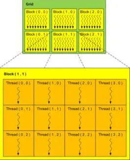
CUDA allows the programmer to define special functions called kernels, such that, when called, are executed N times in parallel by N different CUDA threads [8]. A CUDA program is organized into a host program, consisting of one or more sequential threads running on a host. All threads generated by a kernel define a grid and are organized in blocks. A grid consists of a number of blocks (all equal in size), and each block consists of a number of threads as shown in Figure 2.1 [8]. Each block within the grid is identified through the built-in variable ‘blockIdx’, accessible within the kernel. The dimension of the thread block is accessed through the built-in variable ‘blockDim’. Each thread in a particular thread block is identified using ‘threadIdx’ built-in variable. By using these built in variables each thread determines which element it should process.

(23)

14 2.3 Implementation in CUDA

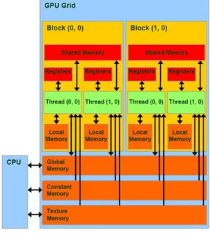
CUDA devices have different types of memories that can be utilized by programmers in order to achieve high performance as illustrated in Figure 2.2 [8]. The global memory is the memory which every thread can access. The data to be processed by the GPU is first transferred from the host memory to the device global memory. Each block has shared memory visible to all threads of the block and each thread has private local memory visible to that thread only. There are also two additional memory spaces accessible by all threads, the constant memory and texture memory. Constant memory provides faster and more parallel data access paths for CUDA kernel execution than the global memory [9]. Texture memory is used to accelerate frequently performed operations and also provides a way to interact with the display capabilities of the GPU.

Figure 2.2: Memory model of GPU

2.3 Implementation in CUDA

The projection algorithm is adopted to find a numerical solution to the Navier -Stokes equation for incompressible fluid flows. In the projection algorithm, the velocity field u* is predicted using the momentum equations without the pressure gradient term. The predicted velocity field u* does not satisfy the divergence free condition because the pressure gradient term is not included in the predictor step. By enforcing the diver-gence free condition on the velocity field at time (t+1), the pressure Poisson equation

(24)

2.3 Implementation in CUDA 15

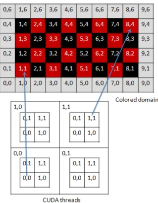
can be derived from the momentum equations as per Thibault et al [10].The pressure-Poisson equation , which is fully implicit is the most time consuming step. It requires convergence to a high degree (mass error), and consumes nearly 80% of the total compu-tational time. Hence it is necessary to port it on a GPU. The discrete pressure-Poisson equation represents a system of linear equations. A number of iterative linear solvers are available, but the selected solver should suit the parallel nature of the GPU. For an implicit algorithm variable at every point is calculated from its neighboring points at the same time step. For the algorithm to run on parallel threads it is necessary that there are no dependencies between variables on different threads. For a second ordered stencil used to solve 2-D Pressure Poisson equation two colors (say red and black) are required to generate two set of points which are independent of each other. The points with same color are processed simultaneously. A thread is created corresponding to every point of a color. The thread-id and block-id provided by CUDA can be used to map a thread to a point of a color and each color is processed sequentially.The Figure 2.3 [9]shows colored domain and thread configuration for processing the points. The threads are mapped to point of one color at a time. For higher-order stencils, more colors will be needed and that will further complicate the code structure.

(25)

16 2.4 Multigrid technique

2.4 Multigrid technique

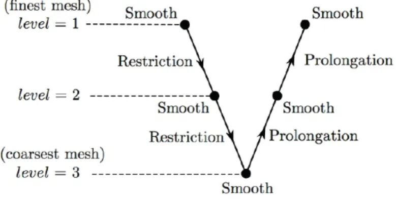
As already mentioned above the Pressure Poisson Equation is the most computationally expensive step in solving the incompressible Navier-Stokes equation hence it is neces-sory to accelerate the convergence rate to reduce the overall runtime of the solver. A geometric multi-grid method is employed for this purpose using a V-cycle, as shown in Figure 2.4.

Figure 2.4: V cycle for 3 levels

Basic Theory

The convergence rate of standard iterative solvers (Gauss-Siedel, Jacobi, SOR) has a tendency to stall or to fail in effectively reducing errors after a few number of iterations. A close inspection of this behaviour reveals that the convergence rate is a function of the error field frequency, i.e. the gradient of the error from node to node. If the error is distributed in a high frequency mode, the convergence rate is fast. However, after the first few iterations, the error field is smoothed out i.e. converted to low frequency and the convergence rate deteriorates. Also the error in a low frequency mode on a finer grid gets converted to a high freqency mode on a coarser grid. Multigrid exploits this fact, thus after a few iterations of smoothening the error in high frequency mode it is transfered to coarser grid to convert low frequency components to high frequency components and smoothen it, hence convergence is achieved with lesser number of iterations. A system of linear equaton can be represented

(26)

2.5 Solution Algorithm for Multigrid on GPU 17

where u is the exact solution of the sytem.If v is an approximate solution to the system of equation the residual r is given by

Av−f =r (2.2)

Also the correction ∆u

∆u=u−v (2.3)

Solving equation 2.1,2.2 and 2.3

A∆u=−r (2.4)

vcorrected =v + ∆u (2.5) as per Briggs et.al[11]

2.5 Solution Algorithm for Multigrid on GPU

The basic steps involved in the multigrid technique are as follows[12]

• Solve on the fine grid using scheme like Gauss Siedel for a few iterations in order to smoothen the high frequency error Compute and store the residual at each fine grid point.

• Interpolate the residual onto the coarse grid .This operation is called restriction. Since for a structured grid every point on the coarse grid has a corresponding point on the fine grid hence values of residuals can directly be transfered. Gener-ally a weighted average of the neighbouring points is considered. The restriction operator I2 1 is calculated as follows I₁2Rij = 1 8[R2i+1,2j+1+R2i−1,2j+1+R2i+1,2j−1+R2i−1,2j−1] 1 4[R2i+1,2j+R2i−1,2j +R2i,2j+1+R2i,2j−1] + 1 2[R2i,2j] [Peiter Wessling][13]

• Solve for the corrections using the equation ∇2_(δP_{) =}₋_R

ij on the coarser grid. These corrections are transfered from coarse grid to fine grid. The corrections for every point in the coarse grid are directly transfered to every point on fine grid, the corrections for other points are determined through interpolation. This operation is called prolongation.

(27)

18 2.6 Pseudocode

• The corrections at the fine grid points are now added to the intermediate solution to provide a better initial guess and further smoothening is done at every level.

• Finally the prolongated correction is added to the intermediate solution on the finest grid and the convergence is checked after smoothening.

• If convergence is not achieved all the above steps are repeated.

2.6 Pseudocode

while error> do

if Level=0 (fine) then

solve for ∇2_P ₌_S

ij

ie smoothen pressure using red-black SOR(GPU)

end if

for Level=1 to Level<maxm do

Restrict residual from Rf ine toRcoarse ie from Level-1 to Level solve for ∇2_(δP_{) =}₋_R _{at each level using restricted R above}

ie smoothen pressure corrections using red-black SOR(GPU)

end for

for Level=maxm to Level=1 do

Prolongate correction fromδPcoarse toδPf ine ie from Level to Level-1 solve for ∇2_(δP_{) =}₋_R _{at each level using corrected initial guesses}

ie smoothen pressure corrections using red-black SOR(GPU) using corrected initial guesses

end for

solve for∇2_P ₌_S

ij using corrected initial guess

ie smoothen pressure using red-black SOR(GPU) using corrected initial guess

(28)

Chapter 3 Governing Equation and Numerical

methodology

3.1 Governing Equation

The basic governing equation for incompressible laminar flow are as follows

Continuity Equation

∇ ·u= 0 (3.1)

Momentum Equation

x-momentum equation

∂u ∂t + ∂(u2) ∂x + ∂(uv) ∂y + ∂(uw) ∂z =− 1 ρ ∂p ∂x + µ ρ ∂2u ∂x2 + ∂2u ∂y2 + ∂2u ∂z2 +ρf x (3.2)

y-momentum equation

∂v ∂t + ∂(uv) ∂x + ∂(v2₎ ∂y + ∂(vw) ∂z =− 1 ρ ∂p ∂x + µ ρ ∂2_v ∂x2 + ∂2_v ∂y2 + ∂2_v ∂z2 +ρf y (3.3)

z-momentum equation

∂w ∂t + ∂(uw) ∂x + ∂(vw) ∂y + ∂(w2₎ ∂z =− 1 ρ ∂p ∂x + µ ρ ∂2_w ∂x2 + ∂2_w ∂y2 + ∂2_w ∂z2 +ρf z (3.4)

(29)

20 3.2 Numerical Methodology for Solving Navier-Stokes Equation

3.2 Numerical Methodology for Solving Navier-Stokes

Equation

The governing equations have been solved numerically by discretizing them temporally and spatially. Spatial discretization has been performed using the finite volume method with a structured orthogonal mesh. The Finite Volume approach has been used since it is easy to extend on non orthogonal grid. Presently non-staggered (collocated) grid arrangement has been used, where the dependent variables are calculated at the cen-troid of the finite volume. But this arrangement can produce non-physical oscillations in the pressure field, the so-called checker-board pressure distribution. When central differencing is used to represent both the pressure gradient term in the momentum equations and the cell-face velocity in the continuity equation, it then happens that the velocities depend on pressure at alternate nodes and not on adjacent ones and the pressure too depends on velocities at alternate nodes. This behaviour is called velocity-pressure decoupling, Patankar[14]. To avoid this decoupling, the momentum interpolation method, first proposed by Rhie and Chow [15] has been used.

The collocated grid arrangement where all the dependent variables are defined at the centroid of the cell P has been used. The four neighboring control volume centers have been defined by E, W, N and S, (for the east, west, north and south neighbours respectively). The face center points e, w, n and s are located at the corresponding face centroid of control volume P. We need to calculate surface vectors for each of the faces of the finite volume and also its volume.

Descretization in Finite Volume

Based on the control volume formulation of analytical fluid dynamics, the first step in the Finite Volume Method is to divide the domain into a number of control volumes. The next step is to integrate the differential form of the governing equations over each control volume. Interpolation profiles are then assumed in order to describe the variation of the concerned variable between cell centroids. The resulting equation is called the discretized or discretization equation. In this manner, the discretization equation expresses the conservation principle for the variable inside the control volume.

(30)

3.2 Numerical Methodology for Solving Navier-Stokes Equation 21

Continuity

Taking an integral over a finite volume for the continuity equation

Z V (ρ∇ ·u)dV = Z S ρu·dS (3.5) Z S ρu·dS ≈ X f=e,w,n,s ρ(u·S)f = X f ρuf ·Sf

where Sf is the surface vector representing the area of the fth cell face and uf is the velocity defined at the face center f. Based on mass conservation the discretized form of the continuity equation can be derived as

X

f

Ff =Fe+Fw+Fn+Fs = 0 (3.6)

where the Ff is the outward mass flux through face f,defined by

Ff =ρuf ·Sf (3.7)

Momentum Equation

Unsteady Term

The unsteady term is descretized after integrating over finite volume ∂ ∂t Z V ρudV ≈ (ρuV) n+1 P −(ρuV) n P ∆t ≈ρVP (u)n_P+1−(u)n_P ∆t (3.8) Convective Term Z V (ρu∇ ·u)dV = Z S ρu(u·dS) (3.9) Summing over all faces

Z S ρu(u·dS)≈X f ρuf(u·S)f = X f Ffuf (3.10)

(31)

Where Ff =uf ·Sf is the convective flux and uf is the value of u at the center of the face.

Z

S

ρu(u·dS)≈Feue+Fwuw+Fnun+Fsus (3.11)

The value of u at the faces can be determined using various convective schemes.

Convective scheme

First order UPWIND scheme

It has been found that the first-order upwind scheme unconditionally satisfies the boundedness criteria and never yields an oscillatory solution, but it has been found to introduce excessive numerical diffusion. Hence second order upwind scheme has been used in the present study. According to first order UPWIND

φf =    φP ifFf ≥0 φnb ifFf <0 (3.12)

Second order UPWIND scheme

In this scheme the values at the face are mainly calculated from the linear interpolation of the values of the neighbouring points. Calculating for east face for Fe ≥0

Figure 3.1: 2nd order UPWIND φe−φP ∆x 2 = φp−φW ∆x φe= 3 2φP − φW 2 φe =    3 2φP − φW 2 ifFf ≥0 3 2φE − φEE 2 ifFf <0 (3.13) Similarly it can be calculated at all other faces.

(32)

3.2 Numerical Methodology for Solving Navier-Stokes Equation 23 Diffusion term −µ ρ Z V ∇ ·[∇U]≈ −µ ρ Z S [∇U]·dS (3.14) ≈ −1 ρ_P X f [µ∇U]_f ·Sf ≈ − 1 ρP X f F_{dU f}n+1 Pressure term Z V −1 ρ ∂P ∂xdV ≈ − 1 ρP Z V ∂P ∂x (3.15) ≈ − 1 ρP Z V (∇P)·nxdV ≈ − 1 ρP X f P_fn+1Sf x

The solution of Momentum Equation

A two step strategy is adopted to solve Navier Stokes equation. In the first step the pressure term is dropped and the equation is solved explicitly for fictitious velocity field called mass velocities u∗ and v∗. In the second step, the corrected pressure field is found out by using the mass velocity obtained from the first step and by solving the pressure Poisson equation. By enforcing the divergence free condition on the velocity field, the Pressure Poisson equation has been derived from the momentum equations as per Julien et al [10]. This corrected pressure field is used to obtain corrected velocity field. The Descretized form of Navier Stokes equation thus obtained is as follows

VpU n+1 p −Upn ∆t + X f F_fnU_fn+ 1 ρ X f F_{dU f}n =−1 ρ X f pn_f+1Sf x (3.16) Vp Vn+1 p −Vpn ∆t + X f F_fnV_fn+1 ρ X f F_{dV f}n =−1 ρ X f pn_f+1Sf y (3.17)

(33)

The Predictor step

Dropping the pressure terms and solving explicitly for mass velocitiesu∗ andv∗ as per equations 3.18 and 3.19 given below.

Vp U_p∗ −Un p ∆t + X f F_fnU_fn+1 ρ X f F_{dU f}n = 0 (3.18) VpV ∗ p −Vpn ∆t + X f F_fnV_fn+1 ρ X f F_{dV f}n = 0 (3.19)

The Corrector step

By definition correction

U_P0 =U_Pn+1−U_P∗ (3.20) Subtracting equation 3.16 and 3.18 , also equation 3.17 and 3.19

VpU 0 p ∆t =− 1 ρ X f pn_f+1Sf x (3.21) Vp V_p0 ∆t =− 1 ρ X f pn_f+1Sf x (3.22) Here the R.H.S of equation can be better understood by simplifying as per equation 3.23 below −X f pfSf ≈ − Z S pdS =− Z V ∇pdV ≈ −VP(∇p)p (3.23)

From the above two equations

U_P0 =−∆t

ρ ∇p n+1

p (3.24)

At the face the equation can be written as U_f0 =−∆t

ρ ∇p n+1

f (3.25)

Also we know that

F_fn+1 =F_fn+F_f0 (3.26) Imposing continuity equation P

f F n+1

f = 0 and solving equation 3.26 yields

X

f

F_f0 =−X

f

(34)

3.2 Numerical Methodology for Solving Navier-Stokes Equation 25

substituting equation 3.27 in equation 3.25 we get the Pressure Poisson equation

X f ∇pn+1_f ·Sf = ρ ∆t X f F_f∗ (3.28) ∆t ρ ∇ 2 P =∇ ·U∗ (3.29)

3.2.1 Solution Algorithm

As per equation 3.18 and 3.19

VpU ∗ p −Upn ∆t + X f F_fnU_fn+1 ρ X f F_{dU f}n = 0 Vp V_p∗−Vn p ∆t + X f F_fnV_fn+ 1 ρ X f F_{dV f}n = 0

Solve explicitly for u∗ and v∗

Solve pressure poisson equation 3.28

X f ∇pn+1_f ·Sf = ρ ∆t X f F_f∗ (3.30)

The pressure poisson equation has been solved implicitly using Gauss Siedel on GPU(Red black) with multigrid . The corrected pressure field is obtained after convergence . Cal-culating Velocity corrections from corrected pressure field using

Vp U_p0 ∆t =− 1 ρ X f pn_f+1Sf x (3.31) Vp V_p0 ∆t =− 1 ρ X f pn_f+1Sf x (3.32) The corrected velocity field is updated

Un+1 =U∗+U0 (3.33)

(35)

26 3.3 Reynolds Averaged Navier-Stokes (RANS) Equations

3.3 Reynolds Averaged Navier-Stokes (RANS)

Equa-tions

Incompressible Navier Stokes in tensor notation is as follows

ρ∂ui ∂t +ρ ∂(uiuj) ∂xj =−∂P ∂xi + ∂ ∂xj (τij) (3.35)

whereτij is shear stress

τij = ∂ ∂x µ ∂ui ∂xj +∂uj ∂xi (3.36) RANS equations for incompressible flows can be derived using the following steps.

• Substitute ui =Ui+ui0 and p=Pi+p0i

• Take the time average over the resulting equations.

• Solve for the averaged quantities (U) and simplify using the statistical properties of turbulent fluctuating quantities (u0 _{= 0) to simplify the resulting equations.}

• Use continuity equation to simplify the equations further.

Taking time average of each term mentioned above as follows

Unsteady term

ρ∂ui ∂t =ρ

∂(Ui+u0i)

∂t (3.37)

By taking time average and using the property of fluctuating components of variables we get ∂(ρui) ∂t = ∂(ρUi+u0_i) ∂t (3.38) = ∂ ρUi+ui 0 ∂t ∂(ρui) ∂t = ∂(ρUi) ∂t (3.39)

(36)

3.3 Reynolds Averaged Navier-Stokes (RANS) Equations 27

Convective term

∂ρujui ∂xj = ∂ ρ Uj+u0j (Ui+u0i) ∂xj (3.40) Taking time average and simplifying

∂ρujui ∂xj = ∂ ρ Uj+u0j (Ui+u0i) ∂xj (3.41) = ∂ ρ UjUi+Uju0_i+Uiu_j0 +u0_ju0_i ∂xj ∂(ρujui) ∂xj = ∂ ρUjUi+ρu 0 ju 0 i ∂xj (3.42)

Pressure Term

∂p ∂xi = ∂(P +p 0₎ ∂xi (3.43) ∂p ∂xi = ∂P ∂xi (3.44)

Stress Term

∂ ∂xj " µ ∂ui ∂xj + ∂uj ∂xj # = ∂ ∂xj  µ ∂(Ui+u0i) ∂xj +∂ Uj+u 0 j ∂xi !  (3.45) = ∂ ∂xj " µ ∂ Ui+u 0 i ∂xj +∂ Uj+u 0 j ∂xi !# = ∂ ∂xj µ ∂Ui ∂xj +∂Uj ∂xi ∂ ∂xj " µ ∂ui ∂xj +∂uj ∂xj # = ∂ ∂xj µ ∂Ui ∂xj +∂Uj ∂xi (3.46) Hence RANS can be now written in the form

ρ∂ui ∂t +ρ ∂(uiuj) ∂xj =−∂P ∂xi + ∂ ∂xj µ ∂Ui ∂xj +∂Uj ∂xi −ρu0_iu0_j

The term ρu0_iu0_j is known as the Reynolds stress tensor comprising three normal stress components and six shear stress components which are not known as a priori and need to be modeled for the closure of the set of governing equations. It is symmetric, hence the number of unknowns are reduced to six (three normal stress components and three shear stress components).

(37)

28 3.4 The k− model

Boussinesq approximation

−ρu0_iu0_j =µt ∂Ui ∂xj + ∂Uj ∂xi −2 3ρδijk (3.47) Substituting above equation provides the closure model for RANS equations. Thus the modeled RANS equations in tensor notation are

∂ ∂xj " µ ∂ui ∂xj +∂uj ∂xj # = ∂ ∂xj (µ+µt) ∂Ui ∂xj +∂Uj ∂xi −2 3ρδijk (3.48)

There are various closure models that have been developed so far. In the present study the k− model which is a two equation model has been used.

3.4 The

k

−

model

The two equation models are found to be complete since they can be used to predict properties of a given turbulent flow with no prior knowledge of turbulent structures. The turbulent viscosityµt is calculated on the basis of turbulent kinetic energy k and dissipation rate . Two separate transport equation are used to solve for k and

k equation ∂k ∂t +Uj ∂k ∂xj =τij ∂Ui ∂xj −+ 1 ρ ∂ ∂xj (µ+µt/σk) ∂k ∂xj (3.49) equation ∂ ∂t +Uj ∂ ∂xj =C1 kτij ∂Ui ∂xj −C2 2 k + 1 ρ ∂ ∂xj (µ+µt/σ) ∂ ∂xj (3.50) µt=ρCµk2/ (3.51) where τij = ∂ ∂xj ∂Ui ∂xj + ∂Uj ∂xi (3.52) Closer coefficients as per Wilcox[16]

(38)

3.5 The solution algorithm for RANS based turbulence models 29

3.5 The solution algorithm for RANS based

turbu-lence models

• The velocity and pressure field is initialized to zero.

• The turbulence parameters are specified through turbulent intensity and viscosity ratio.

• The finite volume descretization of RANS is similar to that of momentum equa-tion ,following is the descretized form of RANS.

Vp U∗−Un p ∆t + ΣF n fUfn+ 1 ρΣF n duf =Vp 1 ρ ∂(µ+µt) ∂y ∂V ∂x − ∂(µ+µt) ∂x ∂V ∂y (3.53) Vp V∗−Vn p ∆t + X F_fnV_fn+ 1 ρ X F_dvfn =Vp 1 ρ ∂(µ+µt) ∂y ∂U ∂y − ∂(µ+µt) ∂x ∂U ∂x (3.54) • The term −2 3 P

kfSf x can be included in the pressure term to get a modified pressure field.

• The extra source terms obtained due to the spatial variation of (µ+µt) denoted asSx and Sy are expressed as follows

Sx =Vp 1 ρ ∂(µ+µt) ∂y ∂V ∂x − ∂(µ+µt) ∂x ∂V ∂y (3.55) Sy =Vp 1 ρ ∂(µ+µt) ∂y ∂U ∂y − ∂(µ+µt) ∂x ∂U ∂x (3.56)

• It has been found that for the current study the contribution of Sx and Sy is negligible.Hence it is has been neglected.

• The equations 4.8 and 4.9 are solved explicitly to find U∗ and V∗

• Solve the pressure equation as per 3.28

X f ∇pn+1_f ·Sf = ρ ∆t X f F_f∗ (3.57)

(39)

30 3.5 The solution algorithm for RANS based turbulence models

• The pressure poisson equation has been solved implicitly using Gauss Siedel on GPU(Red black) with multigrid.

• The corrected pressure field is obtained after convergence.

• Calculating Velocity corrections from corrected pressure field using

Vp U_p0 ∆t =− 1 ρ X f pn_f+1Sf x (3.58) Vp V_p0 ∆t =− 1 ρ X f pn_f+1Sf x (3.59)

• The corrected velocity field is updated.

Un+1 =U∗+U0 (3.60) Vn+1 =V∗+V0 (3.61)

• The value of k and are calculated from their respective transport equation.

Descretized form of k equation

Vp k_pn+1−kn_p ∆t + ΣF n+1 f k n+1 f + 1 ρΣF n+1 dkf +D n+1 k =P r n+1 _(3.62)

Descretized form of equation

Vp n+1 p −np ∆t + ΣF n+1 f n+1 f + 1 ρΣF n+1 df +D n+1 =C1 k n P rn+1 (3.63) Production term P r=Vpµ n t ρ ∂Ui ∂xj + ∂Uj ∂xi ∂Ui ∂xj

Dk is dissipation rate of turbulent K.E

Dk = =CDk3_l/2

D is destruction rate of

D =C2

2

(40)

3.5 The solution algorithm for RANS based turbulence models 31

• Above equations 3.62 and 3.63 are solved using Gauss siedel and iterating till convergence to find updated values kn+1 _and n+1_.

• The eddy viscosity is updated using the following equation

µn_t+1 =ρCµ(kn+1)2/n+1 (3.64)

• This updated value ofµtis used in RANS equations 4.8 and 4.9 at next timestep.

• The problem is solved for steady state.

Source term linearization

• The source term is treated as per Patankar[14].

• For the destruction rate

D_kn+1 ≈Dn_k + ∂Dk ∂k n kn+1−kn (3.65) n+1 ≈n+ ∂ ∂k n kn+1−kn n+1 ≈n+ k n kn+1−kn

• Similarly for dissipation term.

Dn+1 ≈Dn+ ∂D ∂k n n+1−n (3.66) ≈C2f2 k n n+ 2C2f2 k n n+1−n ≈C2f2 k n 2n+1−n

(41)

Chapter 4 Large Eddy Simulation

4.1 Spectral analysis

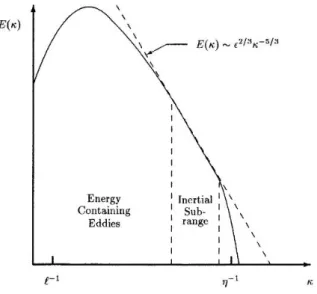
Turbulence consists of a continous spectrum of scales ranging from the largest scale to the smallest scale. The transfer of energy from one scale to other is called energy cascading. As already mentioned large scale fluctuations have a larger dependence on the flow as compared to the small scale fluctuations and these in turn are mostly independent of Large scale statistics, LES mainly exploits this behaviour. Therefore in LES the large scale fluctuations are resolved and small scale fluctuations are modeled. The figure as per [16]shows the energy spectrum for turbulent flows.

(42)

4.2 Filtering 33

The energy spectrum shows that there is range of eddy sizes between largest and smallest scales for which the energy cascade is independent of the energy containing eddies and direct effects of molecular viscosity. Hence for this range the energy trans-ferred by inertial effects dominates and is called as inertial subrange. Since the largest eddies are directly affected by the boundary conditions and carry most of the Reynolds stress they must be computed while the small scale fluctuations are weaker and con-tribute less to Reynolds stresses hence they can be modeled. Therefore the fluctuations upto the inertial subrange are resolved and fluctuations below that are modeled.

4.2 Filtering

In order to filter the small scale fluctuations from the flow filters are used. Using the Gaussian filter function through convolution such that the filtered quantity is given by [17]

u(x, t) =

Z

~u(y, t)G∆x(x−y)dy (4.1) Any variable~u can be described as follows

~

u=u+u0 (4.2)

where u indicates the filtered quantity which is resolved and u0 indicates the subgrid

scaled fluctuation which is modeled. A filter width ∆ is defined such that the fluc-tuations falling above this length scale are termed as large scaled flucfluc-tuations and fluctuations below this length scale are termed as subgrid scaled fluctuations. The filter width is generally taken to be (∆x∆y∆z)1/3.

Filtered Navier Stokes Equation

After applying the Gaussian filter the Navier Stokes equation takes the form ∂ui ∂t + ∂(ui uj) ∂xj =−1 ρ ∂p ∂xi + ∂ ∂xj µ ∂ui ∂xj +∂uj ∂xi +Tij (4.3) where Tij is defined as the sub-grid scale tensor which is given by

Tij =ui uj −uiuj (4.4) The sub-grid scale tensor is modeled using suitable sub-grid scale model. Out of the various models suggested so far, Smagorinsky-Lilly model [5, 6] has been implelmented in the current study.

(43)

34 4.3 Smagorinsky-lilly model

4.3 Smagorinsky-lilly model

Smagorinsky-lilly model is the most widely used eddy viscosity model. It was first proposed by Smagorinsky in 1963. Using Smagorinsky-lilly model the subgrid scale term is modeled as follows

Tij = (Cs∆)2|Sij|Sij (4.5) The Smagorinsky’s model is a sort of mixing-length assumption in which the eddy viscosity is assumed to be proportional to the subgrid scale characteristic length scale ∆x . The eddy viscosity µt is obtained by assuming that the small scales are in equi-librium, so that energy production and dissipation are in balance. The eddy viscosity is calculated from filtered velocity field as follows

µt=ρ(Cs∆)2|Sij| (4.6)

Here|Sij|=

p

2SijSij Where Sij is calculated as follows

Sij = 1 2 ∂ui ∂xj +∂uj ∂xi (4.7)

Cs is defined as smagorinsky constant ∆ = (∆x∆y∆z)1/3.

4.4 Brief discussion on Smagorinsky’s constant

For accurate solution of the flow it is necessory to ensure that the subgrid model dissi-pates correct amount of energy from resolved scale to subgrid scale. The Smagorinsky model is known to be excessively dissipative as per Germano et.al.[18]. Also Large-eddy simulations of transition to turbulence in boundary layers done by Elhady et.al [19] show that during the early stages of transition the Smagorinsky model predicts exces-sive damping of the resolved structures, leading to incorrect growth rates of the initial perturbations. The Smagorinsky’s constant (Cs) plays a vital role in accurate modeling of the subgrid term. Cs does not have a universal value, it is found to change from problem to problem. As per Eswaran and Biswas it can range from 0.07 to 0.2. For a turbulent mixing layer a value of Cs=0.17 or Cs=0.1 has been suggested by Vreman et al.[20]. A higher value of Cs is found to cause excessive damping of large-scale fluc-tuations in the presence of mean shear [21]. Hence in the present work investigations have been done to find the suitable value.

(44)

4.5 Inlet boundary conditions 35

4.5 Inlet boundary conditions

In Reynolds Averaged Navier-Stokes turbulence model the turbulent fluctuations are expressed through the Reynolds stress tensor which is linked to the mean quantities through some turbulence model (k −). However for LES the goal is to explicitly resolve the turbulent fluctuations and inlet conditions cannot be derived from experi-mental results due to unsteady and pseudo random nature of the flow. This problem is more important for spatially developing turbulent flows where the boundary or shear layer thickness changes rapidly. Even for stationary turbulent flows, if realistic initial conditions are not prescribed, the establishment of a fully developed turbulence takes unreasonably long execution time (Smirnov et al. [22]). Hence it is necessory to specify realistic turbulent fluctuations at the inlet as the flow downstream is highly dependent on these conditions. The inlet perturbation propagates throughout the domain and helps trigger the turbulence that is to be captured. The fluctuations have been applied as described in Smirnov et al.[22]. The fluctuations are generated by using turbulence intensity I, a pseudo-random numberα, and the mean streamwise velocity.

U0 =V0 =IαUmean Uinlet =Umean+IαUmean

The random number α is chosen using normal distribution. The mean is specified as zero whereas the variance is specified as unity. The random number hence generated is between -1 and 1. The turbulent intensity is taken around 10%.

4.6 Solution Algoritm for LES

Solve the problem using k− model till steady state is achieved Take the same velocity and pressure field as initial value for LES

VpU ∗₋_Un p ∆t + ΣF n fU n f + 1 ρΣF n duf = 0 (4.8) VpV ∗₋_Vn p ∆t + X F_fnV_fn + 1 ρ X F_dvfn = (4.9)

(45)

36 4.6 Solution Algoritm for LES

The equations 4.8 and 4.9 are solved explicitly to find U∗ and V∗ Solve the pressure equation as per 3.28

X f ∇pn+1_f ·Sf = ρ ∆t X f F_f∗ (4.10)

The pressure poisson equation has been solved implicitly using Gauss Siedel on GPU(Red black) with multigrid . The corrected pressure field is obtained after convergence . Cal-culating velocity corrections from corrected pressure field using

Vp U_p0 ∆t =− 1 ρ X f pn_f+1Sf x (4.11) VpV 0 p ∆t =− 1 ρ X f pn_f+1Sf x (4.12)

The corrected velocity field is updated

Un+1 =U∗+U0 (4.13)

Vn+1 =V∗+V0 (4.14)

The eddy viscosity is calculated based on Smagorinsky-lilly model

µt=ρ(Cs∆)2|Sij| (4.15) Sij = 1 2 ∂ui ∂xj +∂uj ∂xi (4.16) HereSij is calculated based on the corrected velocity field

(46)

Chapter 5 Results and Conclusion

5.1 Laminar Code validation

The laminar code has been validated for lid driven cavity problem. The speed up has been tested separately for GPU and multigrid.

Problem Definition

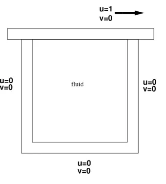
u=0 v=0 u=0_v=0 u=0 v=0 fluid v=0 u=1

(47)

38 5.1 Laminar Code validation

The lid driven cavity is a standard benchmark problem for Navier-stokes equations. It has three stationary wall with a moving lid. The lid has a constant velocity and is assumed to be of infinite length.

Boundary conditions

Wall: u= 0 v = 0 _∂n∂p = 0 Lid: u= 1 v = 0 ∂p_∂y = 0 Re=100 Convergence criteria= 10−7

The problem was solved on GPU using red black Gauss siedel algorithm on single grid. The results were tabulated and the speed up was observed.

Grid size Regular code GPU Speedup 1025X1025 1.41X 10−2 1.78X 10−4 78X 513X513 51.24X 10−5 _{1.44X 10}−5 _35X

257X257 1.44X 10−5 _{3.76X 10}−6 _{15 X}

129X129 7.91X 10−6 _{1.05X 10}−6 _{7.5 X}

Table 5.1: Runtime GPU vs serial code

Code Validation

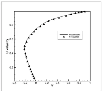
The centerline velocities of components in horizontal and vertical direction were plotted and compared with results obtained from Young et al.[23]

(48)

5.1 Laminar Code validation 39

Figure 5.2: U v/s Y Red Black GS

(49)

40 5.1 Laminar Code validation

The code was extended on multigrid. The results were tabulated and computational effort in terms of work units was compared. For a 512X512 grid the following table shows the variation of work units with levels.

Levels workunits 1 16234321 2 9532673 3 2324576 4 338936 5 92744 6 33088 7 19496 8 17384 9 17312

Table 5.2: Variation of workunits with levels

Grid size GPU single grid code GPU multigrid Speedup 1025X1025 66982312 17656 3793.742X

257X257 16232341 17312 937.63 X

129X129 5309132 15464 343.322 X

65X65 1416243 12232 115.781X

(50)

5.2 Turbulence code validation 41

Figure 5.4: U v/s Y Red Black GS on multigrid

5.2 Turbulence code validation

The turbulent code has been validated for 2D mixing layer problem.

Problem Definition

The mixing layer problem consists of two layers of the same fluid with different velocities respectively.

k

−

model

The k- model has been used to solve the problem.

Boundary conditions

Boundary Conditions Inlet1: u= 1 v = 0 k=ko =o ∂P_∂x = 0 Inlet2: u= 0.25 v = 0 k =ko =o ∂P_∂x = 0 Exit: ∂φ_∂x = 0 (φ =u, v, k, )P = 0

(51)

42 5.2 Turbulence code validation

Figure 5.5: V v/s X Red Black GS on multigrid

Top & bottom boundary : ∂φ

∂y = 0 (φ=u, k, , P) v = 0 ko and o are calculated from I and µr

Turbulence parameters

The turbulence constants are specified as per Wilcox[16]

C1 = 1.44 C2 = 1.92 Cµ = 0.09 σk = 1.0 σ = 1.3 U1 U2 Top Bottom Pressure Outlet

(52)

5.2 Turbulence code validation 43

The turbulent kinetic energy k and dissipation rate are calculated from turbulent intensity I and viscosity ratio. For current problem turbulent intensity I=10% and viscosity ratio µr = 10.

Code Validation

The mid plane velocity was compared with results obtained by Liepmann and Lauffer. The same problem was solved in ANSYS FLUENT and the results were compared.

(53)

44 5.2 Turbulence code validation

Figure 5.8: Comparing mid plane velocity profile

Grid size Regular code GPU Speedup 1025X1025 4.5X 10−2 _{5X 10}−4 _100X

513X513 2.07X 10−3 4.32X 10−5 48X 257X257 2.5X 10−4 1.128X 10−5 22 X 129X129 1.9X 10−5 _{2.15X 10}−6 _{9 X}

(54)

k-5.3 LES model 45

Grid size GPU single grid code GPU multigrid Speedup

1025X1025 113942720 27656 4120X

257X257 32849752 27352 1201 X

129X129 10448440 25484 410 X

65X65 2779032 22232 125X

Table 5.5: GPU single vs multigrid

k-5.3

LES model

The mixing layer problem was solved using LES.The steady state solution obtained for k- is given as initial guess for LES. The filter width ∆x & ∆y is taken equal to the grid size.

Boundary conditions

LES is sensitive to inlet boundary conditions,hence a suitable fluctuating boundary condition has to be given. As already explained in section 4.5 the velocity inlet profile is superimposition of the fluctuation on the mean profile as shown in figure given below.

(55)

46 5.3 LES model

Figure 5.9: Inlet Profile for LES

Determining the length & time scales

Deciding grid size

From the k- model solving RANS equation max = 0.0570 For air ν= 0.000198

Kolmogorov length scale is given by

η = ν3 max 1/4 η= 3.416×10−3

For the energy spectrum to fall beyond sub-inertial range,length scale for LES ≈

(56)

5.3 LES model 47 ∆x= 3.416×10−2 3.416×10−2 =L/Nx Nx =L/3.416×10−2 Nx= 10/3.416×10−2 = 3×102 (5.1) The grid size suitable for the problem is 512×512

.

Deciding timestep

Kolmogorov time scale is calculated

τ = (ν/max)1/2 (5.2)

From the above equation the Kolmogorov time scale is calculated to be of the order of 10−3_{. Due to the CFL constraint on explicit scheme the timestep is taken as 10}−4

(57)

48 5.3 LES model

LES results

The code was first tested for Cs=0.17. The code was found to relaminarize as shown in figure below

Figure 5.10: X-Velocity contour for Cs=0.17

The code was tested for Cs=0.08 . The fluctuations hence obtained at t=40 sec are as per figure below

(58)

5.4 Conclusion 49

Figure 5.11: X-Velocity contour for Cs=0.08

5.4 Conclusion

The first part of this study mainly consists of developing a GPU based solver which uses multigrid algorithm and which is faster than regular solver by several orders of magnitude. Firstly the solver was used to solve the Navier Stokes equation for laminar case and was successfully validated. The solver was then extended to turbulent case. It was first tested for RANS based model, since RANS based models are computationally less expensive as compared to LES . Also from the modeling perspective there is a striking similarity between RANS based model like k- and LES. The k- code was then successfully validated with experimental results obtained by Liepmann & Lauffer.

(59)

50 5.5 Future Scope

In LES it was found that the flow downstream is sensitive to inlet conditions hence realistic fluctuating inlet boundary condition is necessory. Also it was found that the Smagorinsky’s constant does not have a universal value and a high value results in damping of large scale fluctuations Suitable value of Cs for current 2D mixing layer is 0.08.

5.5 Future Scope

The effect of filter width ∆ needs to be tested. The code can be extended to 3D to get better insight into vortex shedding. A general purpose solver based on unstructured grid can be developed. In order to reduce the computational time the code can solved on multiGPU clusters.

(60)

References

[1] Baldwin, B.S. and Lomax H., “Thin-Layer Approximation and Algebraic

Model for Separated Turbulent Flows”, AIAA Paper 78-257., (1978)

[2] Cebeci, T. and Smith, “Analysis of Turbulent Boundary Layers”, A.M.O.,

Academic Press., (1984)

[3] Baldwin, B.S. and Bath, T.J., “A One Equation Turbulence Transport

Model for High Reynolds Number Wall Bounded Flows”, NASA TM 102847., (1990)

[4] _{Spalart P.R. and Allmaras S.R.}, “A One-Equation Turbulence Model for Aerodynamic Flows”, 30th Aerospace Sciences Meeting and Exhibit, Reno,AIAA-92-0439 (January 1992).

[5] Smagorinsky, Joseph, “General Circulation Experiments with the

Primi-tive Equations”, Monthly Weather Review 91 (3): 99164. (March 1963). [6] Lilly,D. K., “A proposed modification of the Germano subgrid-scale closure

method”, Physics of Fluids A 4 (3): 633636. (1992).

[7] S. Pratap Vanka,Aaron F. Shinn,Kirti C . Sahu, “Computational

fluid dynamics using graphics processing units:challenges and opportunities”, ASME,IMECE20 11-65260.(2011).

[8] David B Kirk,Wen-mei W.Hwu, “Programming massively Parallel

Pro-cessors ”, NVIDIA(2011).

[9] S. R. Reddy, J. Sebastian, S.M. Miyyadad, R. Banerjee, N. Sivadasan, “VOF based two-phase flow solver on GPU architecture”,

(61)

52 REFERENCES

[10] Thibault JC, Senocak I, “CUDA Implementation of a Navier-Stokes

solver on Multi- GPU desktop platforms for Incompressible Flows”, 47th AIAA Aerospace Sciences Meeting ,Orlando, Florida(Jan 2009).

[11] William Briggs,Ven Henson,Steve F. McCormick, “A Multigrid

Tu-torial”, Society for Industrial and Applied Mathematics.

[12] John Tannehill,Dale A.Anderson,Richard H.Pletcher,

“Compu-tational Fluid Mechanics and Heat Transfer”,

[13] Pieter Wesseling, “An Introduction to Multigrid Methods”,

[14] Patankar S.V., “Numerical Heat Transfer and Fluid Flow”, Taylor and

Francis(2004)

[15] _{Rhie C.M. and Chow W.L.}, “Numerical Study of the Turbulent Flow Past an Airfoil with Trailing Edge Separation”, AIAA Journal,Vol. 21, No. 11, pp. 1525-1532(1983)

[16] David.C.Wilcox, “Turbulence modeling for CFD”,

[17] Marcel Lesieur, “Turbulence in fluids”

[18] Massimo Germano,Ugo Piomelli,Pervez Moin,William H Cabol,

“A dynamic subgrid-scale eddy viscosity model”, Physics of fluids A 3, 1760(1991)

[19] Nabil M. ElHady, Thomas A. Zang, and Ugo Piomelli, “Application

of the dynamic subgridscale model to axisymmetric transitional boundary layer at high speed”, Physics of fluids 6, 1299(1994)

[20] Bert Vreman,Bernard Geurts,Hans Kuerten, “Large Eddy

simula-tion of the turbulent mixing layer”, J. Fluid Mech 339, 357-390(1997) [21] , “Fluent User guide 6.3”,

[22] A. Smirnov, S.Shi, I. Celik, “Random Flow Generation Technique for

Large Eddy Simulations and Particle-Dynamics Modeling”, Transactions of the ASME-I-Journal of Fluids Engineering 123.2 359-371.(2001)

(62)

REFERENCES 53

[23] D. L. Young, Y. H. Liu, T. I. Eldho, “A combined BEM-FEM model

for the velocity- vorticity formulation of the Navier-Stokes equations in three dimensions”, Engineering Analysis with Boundary Elements 24.(2000) [24] A. F. Shinn, S. P. Vanka, and W. W. Hwu., “Direct numerical

sim-ulation of turbulent ow in a square duct using a graphics processing unit (GPU)”, In 40th AIAA Fluid Dynamics Conference.(2010)

[25] Launder, Brian Edward, and Dudley Brian Spalding, “Lectures in

Large Eddy Simulation of Turbulent Incompressible Flow Using GPU with Multigrid Algorithm