Precision Agriculture
APPLICATION OF A LOW-COST CAMERA ON A UAV TO ESTIMATE MAIZE
NITROGEN-RELATED VARIABLES
--Manuscript
Draft--Manuscript Number:
Full Title: APPLICATION OF A LOW-COST CAMERA ON A UAV TO ESTIMATE MAIZE
NITROGEN-RELATED VARIABLES
Article Type: Manuscript
Keywords: CIR camera; UAV; colorgrams; vegetation indices; maize
Corresponding Author: Martina Corti, Ph.D.
Universita degli Studi di Milano Facolta di Scienze Agrarie e Alimentari ITALY
Corresponding Author's Institution: Universita degli Studi di Milano Facolta di Scienze Agrarie e Alimentari
First Author: Martina Corti, Ph.D.
Order of Authors: Martina Corti, Ph.D.
Daniele Cavalli Giovanni Cabassi Antonio Vigoni Luigi Degano Pietro Marino Gallina
Funding Information: MIPAAF
(D.M n°27335/7303/10) Not applicable
Suggested Reviewers: Toshihiro Sakamoto
Ecosystem Informatics Division, National Institute for Agro-Environmental Sciences [email protected]
Expert of digital camera applied to agriculture S.L. Osborne
USDA-ARS, Northern Grain Insects Research Laboratory [email protected]
Expert in airborne remote sensing of crops H. Noh
Dept. of Biosystems Engineering, Chungbuk National University [email protected]
Expert in the use of digital camera for agricultural application CC Lelong
CIRAD, UMR TETIS [email protected]
Expert in the use of UAV-mounted digital camera in agriculture V Lebourgeois
CIRAD UPR SCA
[email protected] Expert in UAV-based crop monitoring
APPLICATION OF A LOW-COST CAMERA ON A UAV
1
TO
ESTIMATE
MAIZE
NITROGEN-RELATED
2
VARIABLES
3
Martina Corti1, Daniele Cavalli 1, Giovanni Cabassi2, Antonio Vigoni3, Luigi Degano2, Pietro Marino Gallina1
4
1Department of Agricultural and Environmental Sciences - Production, Landscape, Agroenergy, Università degli Studi
5
di Milano; via Celoria 2, 20133 Milano (Italy) 6
2Consiglio per la ricerca in agricoltura e l’analisi dell’economia agraria, CREA-ZA; via Antonio Lombardo 11, 26900
7
Lodi (Italy) 8
3 Sport Turf Consulting-Servizi per l'agricoltura con aeromobili a pilotaggio remoto; Via Cesare Battisti, 19, 20027
9
Rescaldina (MI) 10
Corresponding Author: Martina Corti, [email protected] 11
12
Authors email address: Daniele Cavalli, [email protected]; Giovanni Cabassi, [email protected]; 13
Antonio Vigoni, [email protected]; Luigi Degano, [email protected]; Pietro Marino Gallina, 14
Manuscript Click here to download Manuscript
Manuscript_Martina_Corti_DC.docx
Click here to view linked References
1 2 3 4 5 6 7 8 9 10 11 12 13 14 15 16 17 18 19 20 21 22 23 24 25 26 27 28 29 30 31 32 33 34 35 36 37 38 39 40 41 42 43 44 45 46 47 48 49 50 51 52 53 54 55 56 57 58 59 60 61
2
ABSTRACT
16
The development of small unmanned aerial vehicles (UAVs) and advancements in sensors technology made consumer 17
digital cameras suitable for the remote sensing of vegetation. In this context, monitoring the in-field variability of maize 18
(Zea mays L.), characterized by high nitrogen fertilization rates, with a low-cost color-infrared airborne system could be 19
the basis for a site-specific nitrogen (N) fertilization support system. An experimental field with different N treatments 20
applied to silage maize was monitored during the years 2014 and 2015. Images of the field and reference destructive 21
measurements of above ground biomass (AGB), N concentration in AGB and N uptake were taken at V6 and V9 22
development stages. Classical normalized difference indices and the indices adjusted by crop ground cover were 23
calculated and regressed against the measured variables. Finally, image colorgrams were used to build PLS regression 24
models to explore the potential of band-related information in variable estimation. The best predictors were found to be 25
the ground cover and the adjusted GNDVI: regression equation at V9 resulted in R2 of 0.7 and RRMSE<25% in
26
external validation. Colorgrams did not improve prediction performances due to the spectral limitations of the camera. 27
Therefore, the feasibility of the method should be tested in future research. In spite of limitations of sensor setup, the 28
modified camera was able to estimate maize AGB due to the very high spatial resolution. Since AGB is a robust proxy 29
of N status, the modified camera could be a promising tool for a low-cost N fertilization support system. 30 31 1 2 3 4 5 6 7 8 9 10 11 12 13 14 15 16 17 18 19 20 21 22 23 24 25 26 27 28 29 30 31 32 33 34 35 36 37 38 39 40 41 42 43 44 45 46 47 48 49 50 51 52 53 54 55 56 57 58 59 60 61 62
INTRODUCTION
32
Efficient use of agronomic inputs represents an answer to the increasing attention of public opinion to agriculture 33
intended as a source of environmental pollution, especially referring to nitrogen (N) fertilization that could cause severe 34
air and water pollution with environmental drawbacks (Olfs et al., 2005). A more efficient preservation of resources in 35
agriculture can be gained by modulating external inputs according to the variability in crop response within fields. Both 36
between- and within-field variability can be evidenced with maps describing crop status. Maps could be obtained as 37
outputs of proximal (tractor-mounted) and remote-sensing techniques adopting optical sensors and then used to interpret 38
dynamics of plant N demand during crop growing season, rapidly and accurately substituting destructive and time-39
consuming ground plant sampling and analytical measurements (Olfs et al., 2005). 40
Different satellite-mounted sensors are suitable for monitoring crop N status, providing information at different level of 41
spatial (pixels from 1000 to 0.5 m) and temporal (every 1-44 days) resolution (Mulla, 2013). They usually acquire crop 42
spectral information in the visible (VIS) and near infra-red (NIR) regions of the spectrum allowing calculating common 43
vegetation indices. However, images require post-processing for atmospheric and geometric correction prior vegetation 44
indices calculation (Bastiaanssen et al., 2000). Furthermore, some authors have underlined the limited operational 45
flexibility of such techniques for real time field monitoring or management, due to low spatial resolution of acquired 46
images, long satellite re-visit times, cloud cover and total cost of the service (Berni et al., 2009; Swain et al., 2007). 47
However, nowadays, the improvements of satellite spatial and temporal resolution and the availability of free images 48
renewed the interest in satellite remote sensing for agricultural purposes applied to large surfaces even if the cloud 49
cover is still an issue due to the limited field surfaces and the limited time window suitable for field operations. 50
The limitations of satellite-based crop monitoring have allowed the development and spread of tractor-mounted 51
proximal sensors. These sensors acquire reflectance at two to twenty wavebands in the vegetation indices and NIR 52
range of the spectrum and have their own light source to avoid sunlight dependence. Moreover, tractor-based vegetation 53
indices are used in combination with an N-rich reference filed strip that allows correcting the spectral response to local 54
variables (Raun et al., 2008). 55
Besides the satellite- and tractor-mounted optical sensors, in recent years, new opportunities for crop monitoring were 56
opened by the innovative use of unmanned aerial vehicles (UAVs). These devices, equipped with multispectral digital 57
cameras, can be used to periodically fly over fields and acquire crop spectral information in the VIS and NIR regions in 58
order to calculate vegetation indices at very high spatial resolution (often less than 2 cm). Recent attempts to build crop-59
specific calibration curves between UAV-derived vegetation indices and crop variables are recorded in the literature 60
(Geipel et al., 2016; Huang et al., 2010; Lebourgeois et al., 2008). In fact, UAVs are more flexible in scheduling field 61 1 2 3 4 5 6 7 8 9 10 11 12 13 14 15 16 17 18 19 20 21 22 23 24 25 26 27 28 29 30 31 32 33 34 35 36 37 38 39 40 41 42 43 44 45 46 47 48 49 50 51 52 53 54 55 56 57 58 59 60 61
4 surveys compared to satellite- and tractor- based techniques, putting forward for interesting applications in the 62
following fields: nutrient and water management, weed control, disease and pest detection, estimation of grain yield 63
(Wójtowicz et al., 2016). However, the ability of UAV-mounted sensors to assess vegetation status hangs on images 64
calibration and processing that implies to retrieve reflectance, to compensate for ambient light variation (Kim et al., 65
2008; Noh et al., 2005), and to manage soil background noise (Noh et al, 2005). Nevertheless, UAV-based vegetation 66
indices were successfully regressed against leaf chlorophyll concentration (R2>0.7; Lebourgeois et al., 2008; Miao et
67
al., 2009; Noh and Zhang, 2012), above ground biomass (R2=0.70-0.85; Geipel et al., 2016; Reyniers e Vrindts, 2006),
68
plant nitrogen concentration (R2=0.4-0.8; Geipel et al, 2016; Lebourgeois et al., 2012; Reyners e Vrindts, 2006) and
69
grain yield (R2>0.7; Huang et al., 2010) of different crops.
70
Maize (Zea mays, L.) is the main crop cultivated in the Po plain, Northern Italy, on a surface of 327,632 ha (in 71
Lombardy), with an average production of 11 and 50 t ha-1 of grain and silage-maize, respectively (ISTAT, 2017). Most
72
of the cultivation territory of maize was classified as vulnerable to nitrate leaching (Acutis et al., 2014), and therefore 73
loads of livestock N is limited to 170 kg N ha-1 year-1, while, according to regional legislation, the maximum amount of
74
N that can be annually supplied to maize (including mineral fertilizers) is 280 kg N ha-1 year-1. Therefore, the
75
application of UAV-based crop monitoring at high spatial and temporal resolution, with the aim of mapping crop 76
variability linked to N nutrition, would be crucial to support site-specific fertilization and optimize fertilizer 77
distribution, both in terms of amounts and location. This kind of monitoring is particular interesting since side-dress and 78
top-dress fertilization of maize is applied in a narrow time window, between V6 and V9 development stages. The 79
relative short period suggests adopting UAV-based monitoring tools rather than satellites. 80
Focusing on maize UAV-based monitoring, the survey of literature highlighted that only few experiments were 81
conducted studying the behavior of a low-cost camera for the estimation of maize ground-measured variables. Different 82
authors agreed in finding green band-based vegetation indices as the best predictors for the studied nitrogen-related 83
variables (Osborne et al., 2004; Sakamoto et al., 2012a and 2012b; Rorie et al., 2011a and 2011b). The coefficients of 84
determination ranged between 0.5-0.98 for the estimation of the above ground biomass (AGB), 0.49-0.7 for the 85
estimation of AGB N concentration (Nc) and 0.38-0.59 for the estimation of N uptake (Nu). Furthermore, it must be 86
considered that these experiences were often carried out for one or two years and often at late crop development stages 87
(V13-R6; Ritchie et al., 1993), far from those identified as the best time window for N side-dress fertilization (V6-V9). 88
Finally, even if V6 and V9 development stages were sensed, regression analysis was not performed specifically for 89
those stages but comprehensive of vegetative and reproductive stages, that is including samples taken after maize 90
flowering (Osborne et al., 2004; Sakamoto et al., 2012a and 2012b). 91 1 2 3 4 5 6 7 8 9 10 11 12 13 14 15 16 17 18 19 20 21 22 23 24 25 26 27 28 29 30 31 32 33 34 35 36 37 38 39 40 41 42 43 44 45 46 47 48 49 50 51 52 53 54 55 56 57 58 59 60 61 62
In the cited experiments, few vegetation indices were used to predict crop variables because sensors mounted on UAVs 92
rarely acquired more than three broad bands. However, the most recent image analysis techniques allow expanding 93
band-related information to be used as multivariate predictors of target features. An example is represented by the 94
technique of colorgram extraction that was designed and implemented for food systems by Antonelli et al. (2004) to 95
evaluate food color and defects by multivariate image analysis. It was developed for laboratory applications (Antonelli 96
et al., 2004; Ulrici et al., 2012) and it consisted in the extraction of different color features by deriving new descriptors 97
from the original image, and by projecting them into principal component space. Unluckily, the presented approach has 98
never been used to extract vegetation/canopy signals from aerial images to be used as multivariate predictors of crop 99
variables. If satisfactory, as laboratory applications suggest (Antonelli et al., 2004; Ulrici et al., 2012), this new method 100
would allow deriving information from crop images in a fast, effective and unsupervised way. Colorgrams could be 101
therefore an answer to the main challenge of UAV-based crop monitoring: having fast and reliable image analysis and 102
interpretation (Rasmussen et al., 2016). In this context, such a technique is a very interesting application, especially 103
suited to exploit the potential of band-related information recorded by a low-cost imaging system. 104
We present here a two years-case study where a consumer digital camera, modified to detect a NIR band and mounted 105
on board a UAV, was used to estimate maize AGB, Nc and Nu. To this end, an experimental field with an induced 106
fertilization gradient was used to test the opportunities and limitations of low-cost technology following three strategies. 107
A classical strategy dealt with the calculation of common normalized difference VIs, the Green Normalized Difference 108
Vegetation Index and the Blue Normalized Difference Vegetation Index (GNDVI and BNDVI). The second strategy 109
first considered the estimation of the ground cover (GC), representing the fraction of soil covered by plants. Thereafter 110
two new indices, the BNDVIadj and GNDVIadj were calculated combining the signals coming from pixels belonging to
111
vegetation and the value of GC. In this way, indices adjusted by the GC emphasize the contribution of vegetation both 112
in terms of reflected radiation (they do not consider pixels from soil) and soil coverage. The third strategy involved the 113
extraction of colorgram signals from multispectral images of the field (soil plus vegetation) and of the solely vegetation. 114
Finally, linear and multivariate partial least square (PLS) regression models were applied to estimate maize variables 115
from vegetation indices and colorgrams, respectively. Therefore, based on regression model performances, we tested 116
whether the modified camera could be used to provide low-cost advices for maize N fertilization. 117 1 2 3 4 5 6 7 8 9 10 11 12 13 14 15 16 17 18 19 20 21 22 23 24 25 26 27 28 29 30 31 32 33 34 35 36 37 38 39 40 41 42 43 44 45 46 47 48 49 50 51 52 53 54 55 56 57 58 59 60 61
6
MATHERIALS AND METHODS
118
The UAV survey was carried out on a flat field located in Montanaso Lombardo (Lodi), Italy (45°20’32” N, 9°26’43” 119
E, altitude 80 m asl) during 2014 and 2015 maize growing seasons. The field hosted a multi-year experiment (Cavalli et 120
al., 2014 and 2016) aimed at quantifying N use efficiency of livestock manures applied to silage-maize (Hybrid 121
PR33M15, Pioneer Hi-Bred Italia S.r.l.) followed by an unfertilized catch crop of Italian Ryegrass (Lolium perenne, 122
Lam. Cv Asso). The trial started in spring 2011 and comprised the following six treatments: 1) unfertilised control 123
(CON); 2) ammonium sulphate (AS); 3) unseparated digestate from a mix of cattle slurry and maize (DSMM); 4-5) the 124
liquid (LF) and solid (SF) fractions of DSMM; 6) unseparated anaerobically stored cattle slurry (US). 125
Treatments were applied on plots of 112.5 m2 (15 m long and 7.5 m wide) and were arranged in a randomized block
126
design with four replicates (plots 1-24 in Figure 1). Blocks were separated each other by ten meters strips. Every year, 127
from 2011 to 2014, manures and AS were applied to the same plots at similar NH4-N rates (on average 140 kg NH4-N
128
ha-1). Differences in applied organic N and in N use efficiency among fertilizers provided a wide range of variability in
129
plant available N within the field. For this reason, the field was chosen to be surveyed by the UAV mounting the 130
modified camera, for calibration purposes. In spring 2015 fertilizations were suspended in order to quantify residual N 131
effects of previous fertilizations (Cavalli et al., 2016). An additional treatment of ammonium sulphate (AS150; 150 kg N
132
ha-1) was applied in half of the original AS plots in order to compare apparent N recovery of 2014 with that of previous
133
years (plots 25-28 in Figure 1). Furthermore, three other treatments of mineral fertilizers were added to the original 134
design to rise further variability of plant available N. Additional treatments comprised ammonium sulphate applied at 135
35 and 70 kg N ha-1 (AS
35 and AS70), and calcium nitrate applied at a rate of 150 kg N ha-1 (CAN150). They were applied
136
on plots of 60 m2 (8 m long and 7.5 m wide) arranged in a randomized block design with four replicates, and located in
137
the strips between blocks of the original experiment (plots 29-40 in Figure 1). Finally, during 2015, eight unfertilized 138
areas of about 1.5 m2 outside the experimental plots were sampled in order to further increase variability in the collected
139
samples (points 41-48 in Figure 1). 140
FIGURE 1, HERE. 141
Crop sampling and analysis
142
Plants were sampled at maize phenological stages V6 and V9 (six and nine fully expanded leaves; Ritchie et al., 1993) 143
in both years, corresponding to 18 July and 1 August 2014 and 3 July and 13 July 2015, respectively. Aboveground 144
biomass (AGB) was estimated by collecting 15 whole plants per plot (three plants per row of the five inner rows of each 145
plot). Plants were oven dried (105°C) until constant weight in order obtain AGB values on a dry matter (DM) basis. 146
Samples were ground with a ZM 100 centrifugal mill equipped with a sieve of 0.2 mm mesh (Retsch Gmbh & Co., 147 1 2 3 4 5 6 7 8 9 10 11 12 13 14 15 16 17 18 19 20 21 22 23 24 25 26 27 28 29 30 31 32 33 34 35 36 37 38 39 40 41 42 43 44 45 46 47 48 49 50 51 52 53 54 55 56 57 58 59 60 61 62
Haan, Germany). Total nitrogen concentration in AGB (Nc; g N 100 g DM-1) was determined by dry combustion using
148
a ThermoQuest NA1500 elemental analyser (Carlo Erba, Milano, Italy). Nitrogen uptake of maize (Nu; g N m-2) was
149
calculated by multiplying AGB (g DM m-2) by Nc.
150
Image acquisition and processing
151
A consumer digital camera Canon® Powershot SX260 HS was converted to a color-infrared camera (CIR) by removing 152
the infrared blocking filter and adding a Super Blue IR filter (www.publiclab.com). Therefore, the red channel was used 153
to acquire reflectance in the NIR, while the blue (B) and green (G) channels remained the same. After the modification, 154
the spectral resolution of the camera was tested in laboratory conditions by single waveband measurements in the range 155
between 400 and 800 nm, every 10 nm using a monochromator equipped with a Xenon lamp. Images were acquired in a 156
dark room, at a distance of 7 cm from the light source, with the monochromatic ray normally striking the camera sensor. 157
The camera was manually set up to eliminate saturated values in any band using the following settings: focus, 8.0, 158
exposure time 1/60 s and sensitivity ISO100. 159
The CIR camera was mounted on board a prototype UAV coaxial octocopter. The UAV was made of carbon fiber with 160
a maximum payload of 12 kg and was equipped with a GNSS (Global Navigation Satellite System) NEO-M8N (u-blox, 161
Thalwil, Switzerland) and double gimbal platform for mounting the camera. 162
Images were acquired immediately before plant sampling, under clear sky conditions, between 11:00 and 13:00 a.m. 163
solar time, assuring no variation in the incident light angle, and under homogeneous soil wetness level. The UAV 164
survived the field at a speed of 5 m s-1 and an altitude of 35 m above ground level. The flight plan guaranteed a 75%
165
forward and sideward overlap between images. 166
Images were recorded in 8-bit JPEG format with the camera pointing to the nadir direction. The JPEG file format was 167
chosen because JPEG file dimensions were more feasible for UAV-applications at farmer level. Furthermore, geometric 168
and vignetting corrections were done by the original Canon firmware. The camera was set up with autofocus mode, 169
maximum wide angle, a fixed ISO value of 200, 1/1250 s shutter speed. The automatic aperture stop resulted to be the 170
same each flight (3.625) due to the short flight duration time and optimal light conditions. The output images were 12.1 171
MP (Mega pixel), 3-band 8-bit per band JPEG files, with a spatial resolution of 1.5 cm. Orthomosaics of the images 172
were made, separately for each day of acquisition, using the software Pix4Dmapper (Pix4D SA, Lausanne, Switzerland) 173
that performed a 3D points-based stitching. No radiometric calibration was carried out at this step. Areas belonging to 174
ground points were extracted from orthomosaics, obtaining images representative of the sampled areas of the field. In 175
the year 2014 and 2015, the area corresponding to the inner five rows of each plot was extracted. In addition, areas 176
corresponding to points 41-48 was selected close to ground sample using GPS coordinates as reference. Thus, given the 177 1 2 3 4 5 6 7 8 9 10 11 12 13 14 15 16 17 18 19 20 21 22 23 24 25 26 27 28 29 30 31 32 33 34 35 36 37 38 39 40 41 42 43 44 45 46 47 48 49 50 51 52 53 54 55 56 57 58 59 60 61
8 different size of some plots in 2014 and 2015 and that of additional points out of plots, extracted images had different 178
size. A white tile positioned in each plots was used to calculate the reflectance values of the images, by normalizing 179
pixel intensities by the value of the white reference, after subtracting the black reference. Black reference consisted by 180
sampling the lowest intensity value recorded by all the images of the same flight. 181
Vegetation indices
182
The Blue Normalized Difference Vegetation Index (BNDVI) and the Green Normalized Difference Vegetation Index 183
(GNDVI) were calculated, for each pixel of extracted images according to the following equations: 184
Classical NDVI-based indices=NIR-Band
NIR+Band Eq. 1
Were Band stands for the blue band in the case of BNDVI and green band in the case of GNDVI. Indices were 185
calculated using MATLAB version R2014b (MathWorks, Natick, MA). 186
The Otsu algorithm (Otsu, 1975) was used to identify, within each image, pixels belonging to vegetation. Segmentation 187
was based on BNDVI or GNDVI providing, in both cases, a mask of the vegetation (Maskveg). The BNDVI-based
188
segmentation strategy resulted in a better separation between soil and vegetation, while GNDVI did not discriminate 189
soil shadows from leaves, resulting in undersegmentation. Therefore, the canopy ground cover (GC), representing the 190
fraction of total pixels classified as vegetation, was calculated using Maskveg based on BNDVI.
191
After GC calculation, two additional indices were derived from BNDVI and GNDVI in order to give a zero weight to 192
pixels classified as soil, and thus emphasize the signal coming from vegetation. The two indices, BNDVIadj and
193
GNDVIadj, were calculated using following the equation:
194 𝑉𝐼𝑎𝑑𝑗 = ∑𝑛𝑖=1∑𝑚𝑗=1𝑉𝐼𝑖𝑗× 𝑀𝑎𝑠𝑘𝑣𝑒𝑔 𝑖𝑗 ∑𝑛𝑖=1∑𝑚𝑗=1𝑀𝑎𝑠𝑘𝑣𝑒𝑔 𝑖𝑗 × 𝐺𝐶 Eq. 2
where VIij and Maskveg ij are the value of the vegetation index (BNDVI or GNDVI) and the classification value (zero or
195
one) of the pixel ij, respectively, while n and m represent the number of rows and columns of the image. For both 196
indices, the classification mask Maskveg was based on BNDVI values.
197
Image colorgrams
198
Colorgrams were constructed following the method proposed by Antonelli et al. (2004) with the aim of extracting the 199
most complete information related to image color. Each colorgram is a linear signal that sequentially combines 200
frequency distributions of the following band-related information: 1) intensity values of the three channels NIR, G, and 201
B (region 1-768); 2) lightness, calculated as the sum of the three channels intensities (region 769-1024); 3) relative 202
channel intensities, calculated as the ratio between channel intensity and lightness (region 1025-1792); 4) values of the 203
original channels after projection in the hue space (region 1793-2560). Finally, scores values derived from a three-PCA 204 1 2 3 4 5 6 7 8 9 10 11 12 13 14 15 16 17 18 19 20 21 22 23 24 25 26 27 28 29 30 31 32 33 34 35 36 37 38 39 40 41 42 43 44 45 46 47 48 49 50 51 52 53 54 55 56 57 58 59 60 61 62
model applied to the image are calculated and joined to the colorgram signal (region 2561-4864). The model is applied 205
on the raw, the mean centered and the autoscaled spectra matrices because the process is unsupervised, without any 206
prior knowledge on which pretreatment performs better than others (Antonelli et al., 2004). Loadings and eigenvalues, 207
derived from the PCA model, are added as the final part of the signal (region 4865-4900). In this work, we introduced a 208
standardization procedure not used in the original paper. The frequency distributions forming each colorgram were 209
divided by the number of pixels of each image. In the original method (Antonelli et al., 2004) no standardization was 210
required because images had the same dimensions, however, in this work, we worked on both full and segmented 211
images (i.e. considering only pixels classified as vegetation). Therefore, the number of pixels used in the procedure 212
differed among images, and standardization was needed. 213
Standardized colograms of whole images (CLRG) and segmented images (CLRGveg) were built using MATLAB and an
214
ad-hoc self-built function. Figure 3 shows the resulting signals. 215
Statistical analysis
216
Analysis of variance (ANOVA) was carried out, separately for each year and sampling date, to test the significant effect 217
of treatment on AGB, GC and GNDVIadj. The ANOVA model considered the treatment as a fixed factor and block as
218
random. The homogeneity of variances was evaluated using the Levene test (P<0.05). Significant effects of treatments 219
are reported when the P is below 0.05. Treatments were grouped according to the HSD Tukey test (P<0.05). All 220
ANOVAs were performed using the SPSS procedure UNIANOVA (SPSS Versions 24.0.0). 221
The aim of mean separation was to evaluate whether treatments statistically affected measured variables and vegetation 222
indices in a similar way. Therefore, we were interested in assessing if vegetation indices could be able to discriminate 223
among statistically different means of measured variables originated from different available N rates (originating from 224
both yearly added N fertilizers or mineralized residual organic N). 225
Linear regression models were built, separately for each crop development stage V6 and V9, to estimate AGB, Nc and 226
Nu from the six predictors: BNDVI and GNDVI, GC based on BNDVI and GNDVI, and indices BNDVIadj and
227
GNDVIadj.
228
Multivariate analysis was used to predict AGB, Nc and Nu from standardized colorgrams. Partial least square 229
regression models (PLS) were built, separately for V6 and V9, using CLGR or CLGRveg colorgrams.
230
The entire dataset (24 and 48 sampling points for 2014 and 2015, respectively) was divided into a calibration and a 231
validation dataset. The calibration dataset (48 samples) comprised all samples from the 2014 campaign (24 samples) 232
and samples from the 2015 campaign belonging to plots 27-40 and sampling points 41-48 (24 samples). The remaining 233 1 2 3 4 5 6 7 8 9 10 11 12 13 14 15 16 17 18 19 20 21 22 23 24 25 26 27 28 29 30 31 32 33 34 35 36 37 38 39 40 41 42 43 44 45 46 47 48 49 50 51 52 53 54 55 56 57 58 59 60 61
10 24 samples of the year 2015 were used as validation datasets. The resulting datasets partially minimized the occurrence 234
of autocorrelation between samples taken on the same plot in the two consecutive years. 235
Finally, linear and PLS regressions models were built on the pooled data of the two phenological stages by joining the 236
dataset of V6 and V9, resulting in a global dataset of 96 and 48 samples for calibration and validation, respectively. 237
These models provided prediction of maize variables for a time window suitable for side-dress N fertilization. 238
The statistics coefficient of determination (R2) and relative root mean squared error (RRMSE; %) were used to judge
239
the performances of linear and PLS regression models, both applied to the calibration and validation datasets. 240 1 2 3 4 5 6 7 8 9 10 11 12 13 14 15 16 17 18 19 20 21 22 23 24 25 26 27 28 29 30 31 32 33 34 35 36 37 38 39 40 41 42 43 44 45 46 47 48 49 50 51 52 53 54 55 56 57 58 59 60 61 62
RESULTS
241Camera sensitivity
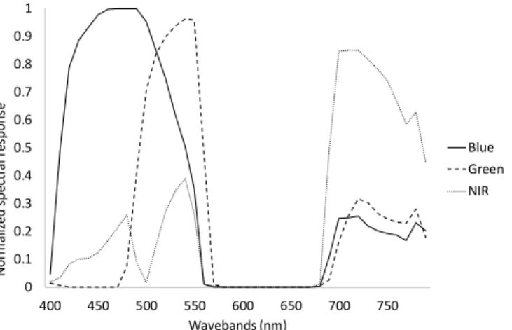
242 FIGURE 2, HERE. 243Sensitivity test on the CIR camera showed that the blue channel had a peak at 460-490 nm, centered at the blue 244
wavelengths of 460 nm. However, blue pixels acquired also wavelengths from 400 to 560 nm, covering part of the 245
green region of the visible spectrum. The green channel resulted narrower than the blue one and it was sensible to the 246
wavelengths from 470 to 570 nm with a peak on the green region (540-550 nm). Finally, the red channel, after 247
modification, recorded the NIR wavelengths going from 680 to 800 nm. The removal of the NIR filter caused the 248
overlapping of the three channels in the NIR region: in fact, also the blue and the green channel recorded wavelengths 249
from 680 to 800 nm. The NIR channel, finally, acquired a small portion of the visible light in the blue and green regions 250
of the spectrum due to the applied superblue filter. 251
Measured datasets
252
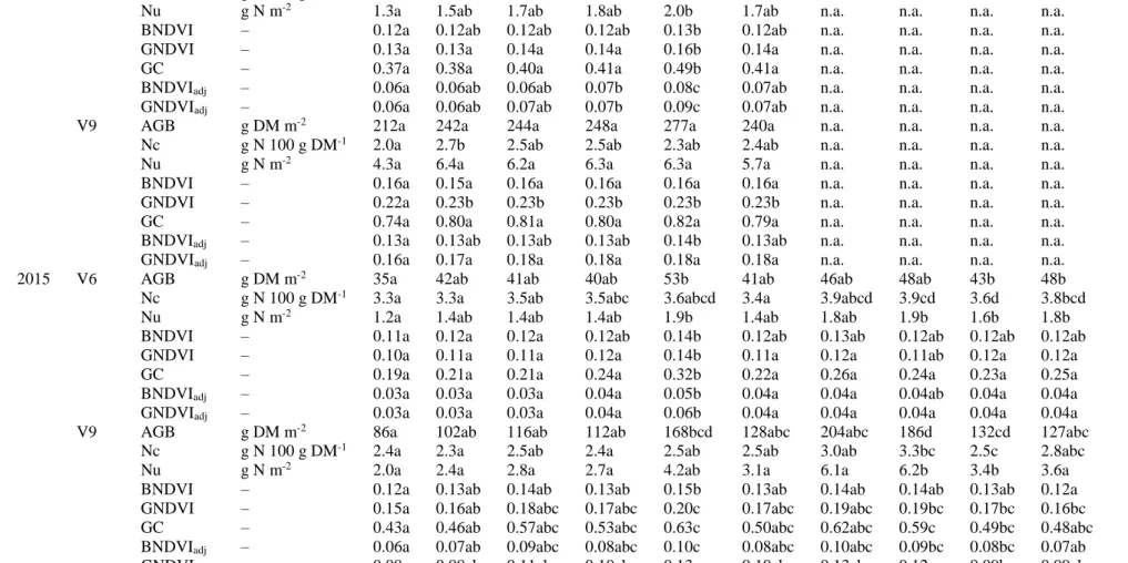
During each season, maize AGB and Nu markedly increased from V6 to V9 (Table 1), while N in AGB tissues was 253
progressively diluted, as confirmed by lower Nc values at V9 compared to V6 (Table 1). Variability of measured 254
variables was narrow at V6, and it was similar for the years 2014 and 2015, suggesting that fertilizer N effects occurred 255
at later stages of crop development in both years. Indeed, despite variable applied N fertilization levels, only few 256
significant differences (P<0.05; Table 1) in AGB and Nu were found among treatments. In particular, AGB was higher 257
in SF compared to CON, AS and DSMM in 2014, while in 2015, only SF and chemical fertilizers added at a rate of 150 258
kg N ha-1 (AS
150 and CAN150) significantly enhanced maize AGB compared to CON. A similar pattern was observed for
259
Nu and Nc in 2015, while in 2014 Nc did not significantly varied among treatments. 260
Conversely, when crop reached V9, higher variability was measured in 2015 than in 2014, in agreement with the wider 261
range of applied N rates. ANOVA confirmed that treatments in 2015 significantly (P<0.05) affected both crop biomass 262
and Nu (Table 1). Conversely, maize did not responded significantly to N fertilization in 2014, when all treatments 263
showed similar AGB and Nu. 264
TABLE 1, HERE. 265
Vegetation indices
266
Vegetation indices, both classical (BNDVI and GNDVI) and adjusteded (BNDVIadj and GNDVIadj), and GC increased
267
during crop development from V6 to V9, according to the increase in AGB and plant N uptake (Table 1). 268 1 2 3 4 5 6 7 8 9 10 11 12 13 14 15 16 17 18 19 20 21 22 23 24 25 26 27 28 29 30 31 32 33 34 35 36 37 38 39 40 41 42 43 44 45 46 47 48 49 50 51 52 53 54 55 56 57 58 59 60 61
12 In general, the effect of treatments on vegetation indices and GC was similarly to that on AGB and Nu, as confirmed by 269
homogeneous groups reported in Table 1. However, at V6 in 2015, grouping based on vegetation indices and GC did 270
not differentiate between treatments receiving fertilizers at a rate of 150 kg N ha-1 and CON, as grouping for AGB and
271
Nu suggested. 272
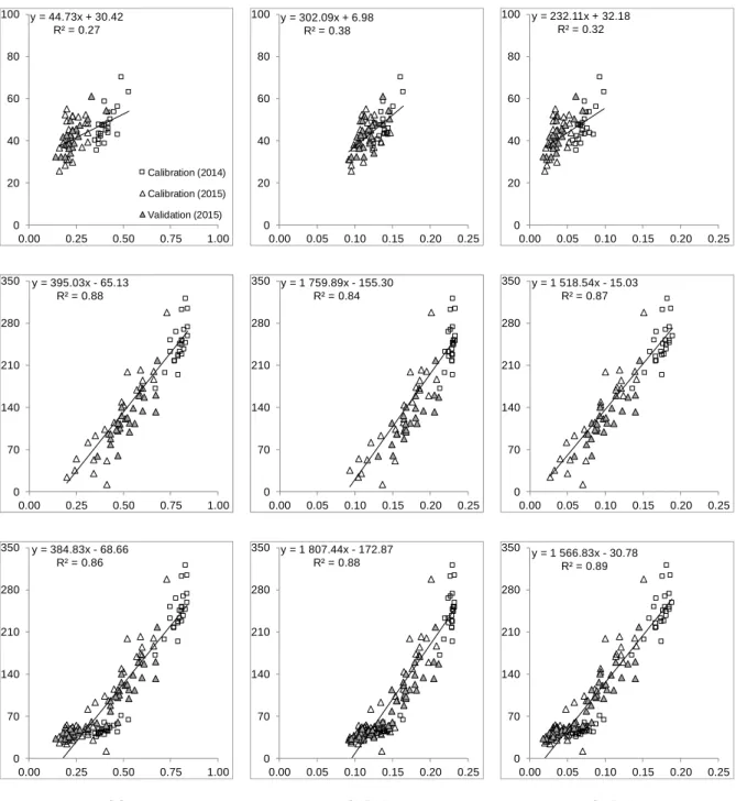
At V9, all indices showed a relationship with AGB characterized by a linear response followed by a flat response, 273
suggesting a saturation of the blue and green channels at high AGB levels (Figure 3 for GNDVI and GNDVIadj).
274
Optimization of a simple linear-plateau model confirmed that lack of response occurred at AGB levels higher than 220 275
g DM m-2.
276
Correction of BNDVI and GNDVI by GC allowed increasing the slope of the relations between the indices and AGB, 277
and increasing the value of the plateau by about 10% compared to corresponding uncorrected indices, and thus to extent 278
the linear relationship (Figure 3). 279
Linear PLS Regression models
280
Division of collected data into a calibration and a validation dataset provided sufficient variability in measured variables 281
in both generated sets (Table 2). In addition, the validation sets were always included into calibration limits, ensuring to 282
respect the domain of applicability of the calibrated models. 283
Regressions between vegetation indices and Nc were not significant at both phenological stages (Table 3). The lack of a 284
strong biochemical relationship between the broad bands collected by the CIR camera and Nc resulted in poor 285
calibration models when the range of variation explored by the measured data was not wide enough. Indeed, joining the 286
datasets of the two phenological stages (V6+V9) enabled improving calibration performances, obtaining significant 287
regression models and acceptable validation errors (RRMSE <18%). Even if similar calibration performances were 288
found among all the tested indices, those adjusted by the GC gave better results in validation, without visible difference 289
among GC, BNDVIadj and GNDVIadj. The fact that Nc was successfully estimated due to the effect of nitrogen
290
treatments on AGB and not thanks to the different levels of greenness recorded by the camera was confirmed by the 291
similar results in the external validation between vegetation indices and colorgrams (Table 3). 292
TABLE 2 AND 3, HERE. 293
The calibrated regression models for the estimation of Nu at V6 gave poor results (R2<0.2), probably due to the low
294
capability of the camera in recording low AGB levels at early development stages. In fact, also AGB estimation gave 295
poor results at V6 (Table 3). The good performances in calibration shown by the PLS regression models built using 296
colorgrams as AGB predictors seemed contradictory. In fact, very high coefficients of determination (R2>0.8) and
297 1 2 3 4 5 6 7 8 9 10 11 12 13 14 15 16 17 18 19 20 21 22 23 24 25 26 27 28 29 30 31 32 33 34 35 36 37 38 39 40 41 42 43 44 45 46 47 48 49 50 51 52 53 54 55 56 57 58 59 60 61 62
RRMSEs less than 10% were obtained in calibration. Despite these good results, in the external validation (R2<0.5 and
298
RRMSE ~ 20%) the PLS models based on colorograms proved not to be robust. 299
Very satisfactory results were found in AGB estimations performed at V9. Similar performances were found among 300
classical vegetation indices and the indices adjusted by the GC in terms of R2 and RRMSE of calibration: 0.85 and
301
17.5% on average, respectively. PLS regression models built on colorgrams led to slightly better results in calibration. 302
The similar performances of the colorgrams of the entire image and of vegetation only were expected, because at V9 the 303
contribution of soil pixels to the canopy signal was minimal due to the high GC of maize canopy. External validation 304
proved that models based on GC and indices adjusted for the vegetation fraction were very similar to each other and the 305
best performing (in particular GC and GNDVIadj) compared to the classical vegetation indices (Figure 3), BNDVI and
306
GNDVI, and colorgrams. 307
Finally, the best results were found when the V6 and V9 datasets were joined. The high variability explored (Table 2) 308
led to the best calibration models for all the tested indices. The higher sensibility of the indices to the variation of AGB 309
levels was confirmed and Nc estimation greatly improved. 310 FIGURE 3, HERE. 311 1 2 3 4 5 6 7 8 9 10 11 12 13 14 15 16 17 18 19 20 21 22 23 24 25 26 27 28 29 30 31 32 33 34 35 36 37 38 39 40 41 42 43 44 45 46 47 48 49 50 51 52 53 54 55 56 57 58 59 60 61
14
DISCUSSION
312
At first, the spectral response of the camera after the modification was studied. This step was needed in order to 313
understand the feasibility of the camera for crop monitoring in terms of accuracy of the band-related information 314
acquired by the sensor. In agreement with previous studies on modified digital cameras (Pauly, 2014 and 2016) it was 315
found out that the CIR camera suffered of channel overlapping (Figure 2). This caused the resulting channel intensities 316
to be correlated and therefore, band-related information, as acquired by the CIR camera, was not the most relevant 317
feature at the basis of the capacity of the camera to discriminate among different AGB, Nc and Nu levels. Indeed, PLS 318
models built using colorgrams as predictors of AGB, Nc and Nu, even with good calibration performances, did not 319
improve validation performances compared to classical vegetation indices and to indices adjusted by GC (Table 3). This 320
result supported the hypothesis that features of the camera other than band-related information mostly contributed to 321
maize variable predictions (Table 3), since colorgrams were thought as a technique to extract redundant band-related 322
information (Antonelli et al., 2004). Indeed, the ability of the image-based vegetation indices to assess vegetation status 323
relied on the strong relationship existing between the indices and canopy GC that was related, in turn, to AGB (Hunt et 324
al., 2010; Li et al., 2010; Zhou et al., 2018), at least in early stages of crop development. Imaging sensors basically 325
acquire information about soil coverage by canopy: as GC increases, the portion of vegetation pixels increases until 326
canopy closure (that usually occurs after V9, in maize). Thus, in the time window from emergence to canopy closure, 327
very high spatial resolution imagery could play a role in the assessment of AGB variability even if the sensors used are 328
characterized by low radiometric resolution and overlapping channels. 329
In this context, the difficult estimation of Nc at V6 and V9 (Table 1 and 3) was expected because vegetation indices 330
were known to be affected by the confounding effects of changings of canopy architecture (Eitel et al., 2008). 331
Moreover, our best results, obtained by combining data of V6 and V9 (Table 3), were similar to those obtained in 332
comparable experiments on maize conducted with airborne multispectral imagery (Osborne et al., 2004; Vergara-Dìaz 333
et al., 2016). In both cited experiments, linear regression models to predict Nc based on GNDVI performed better than 334
those based on red NDVI, and provided similar prediction performances in the two experiments (R2 0.23-0.49) when
335
maize was at phenological stages V14-R1 (flowering). The lack of channel signal accuracy of the CIR camera used in 336
our experiment was probably balanced by the high range of variation of the measured Nc (1.69-4.07% for the V6+V9 337
dataset; Table 2) that allowed gaining similar performances. 338
As expected, estimation of AGB gave the best results while the goodness of Nu estimation depended on the 339
performances in the estimation of both, AGB and Nc. Therefore, we will focus our discussion on AGB estimation. The 340
ANOVA highlighted that differences in AGB among treatments were sensed by all indices quite well (Table 1), 341 1 2 3 4 5 6 7 8 9 10 11 12 13 14 15 16 17 18 19 20 21 22 23 24 25 26 27 28 29 30 31 32 33 34 35 36 37 38 39 40 41 42 43 44 45 46 47 48 49 50 51 52 53 54 55 56 57 58 59 60 61 62
irrespective to the saturation phenomenon that probably affected the vegetation index at high AGB levels (Figure 3). 342
The fact that treatment groups based on measured maize variable and vegetation indices agreed, together with 343
prediction performances for the V9 and V6+V9 datasets (Table 3) led to the conclusion that the modified digital camera 344
could be a valuable tool in identifying the within-field variability of maize in the time window from V6 to V9, suitable 345
for N fertilization. 346
However, results at V6 suffered from problems of image acquisition in the 2015 campaign. Indeed, the 2015 dataset, 347
that constituted part of the calibration dataset (Figure 3), was characterized by a narrow variation in GC (0.19-0.23) 348
against a wide range of measured AGB (28-55 g DM m-2). Therefore, the error in the estimation of AGB was probably
349
due to some blurred images collected during the 2015 survey, as confirmed by individually visual inspection of 350
acquired images. These images prevented the algorithm of segmentation working properly and maize plants resulted 351
oversegmented and consequently, the GC underestimated. Another issue that could have played a role is the correlation 352
observed among the collected bands (Figure 2). Pauly (2016) noted that it caused a more difficult discrimination 353
between leaves and soil when using modified cameras that are affected by channel overlapping, as in this case. The 354
described factors probably affected the estimation performances at V6, where the confounding effects of soil and 355
shadows were higher than at V9 (Sripada et al., 2005). An example of the segmentation procedure is provided in figure 356
4. This reason could explain the low performances at V6 of the indices and, in particular, the worse performance of the 357
GC and of the adjusted indices if compared to the classical BNDVI and GNDVI that were not affected by the 358
segmentation procedure. 359
FIGURE 4, HERE. 360
The most satisfactory results were obtained at V9. Indeed, good quality images in both years guaranteed the extraction 361
of reliable vegetation indices; in addition, the high range of the measured AGB at V9 was markedly suited for 362
calibration purposes. High R2 (0.68-0.71; Table 3) and low RRMSE (22-24%) were gained in validation for GC and
363
adjusted indices BNDVIadj and GNDVIadj. The better performances of GC and of the adjusted indices could be
364
explained by the fact that the GC had a more linear response to AGB than the classical indices themselves (Figure 3). 365
Therefore, the use of GC as a weighting factor allowed linearizing responses of the vegetation indices to the AGB 366
levels. Accordingly, the distributions of the indices weighted for GC were more similar to the distribution of AGB 367
values and less affected by saturation: GNDVI saturated at 234 g DM m-2 while GNDVI
adj saturated at 250 g DM m-2,
368
similarly to GC. Our results in AGB estimation were very positive compared to those found in multispectral imagery-369
based experiments on maize, even done with airborne sensors specific for vegetation monitoring: 0.18-0.65 of R2
370
(Osborne et al., 2004) vs 0.80-0.88 of our experiment. Finally, experiments with digital camera mounted on ground 371
stations (Sakamoto et al., 2012a and 2012b) gave comparable results (R2=0.79-0.99 obtained by non-linear fitting and
372 1 2 3 4 5 6 7 8 9 10 11 12 13 14 15 16 17 18 19 20 21 22 23 24 25 26 27 28 29 30 31 32 33 34 35 36 37 38 39 40 41 42 43 44 45 46 47 48 49 50 51 52 53 54 55 56 57 58 59 60 61
16 by vegetation indices other than NDVI and GNDVI). The better results could be ascribed to the wide window of the 373
explored maize development stages (the entire season), to the good quality of the images, more manageable form a 374
ground station compared to airborne sensors, to the quality of the camera spectral response and to the different fitting 375
methods and vegetation indices studied. None of the cited literature gave information about performance in validation 376
of the proposed equations. Even in the cases of models based on indices acquired with hyperspectral imaging sensors 377
characterized by high spectral and radiometric resolution (Cilia et al., 2014; Perry and Roberts, 2008), calibration 378
results were from worse to comparable with R2 of 0.45 (V14) and 0.77 (V10). The fact that the estimation of AGB was
379
reliable and comparable to those obtained with more refined approaches, confirmed the promising results of the 380
proposed method, in spite of the limitations of our sensor setup. However, some aspects must be taken into account for 381
future research to fully explore the feasibility of the use of a modified low-cost camera for maize monitoring: the time 382
window going from V6 to V9 should be adequately investigated in order to provide a unique calibrated equation 383
suitable for the estimation of maize AGB and Nu at the time of N fertilization. More attention should be paid for image 384
quality in terms of absence of blurred images, a calibrated reference panel should be used to get more reliable image 385
intensity values (Pauly, 2014) and RAW (native image file format) images acquisition should be considered (Verhoeven 386
et al., 2010). Finally, since the colorgram-based estimations were affected by overfitting, probably due to redundancies 387
in band-related information as acquired by the CIR camera, in future research, the feasibility of the method could be 388
studied by testing it on ground-based images taken by an RGB camera or by a multispectral narrow-band camera, to 389
avoid channel overlapping and the related issues. In fact, the colorgram approach that offers an unsupervised image 390
processing for object classification and prediction of object properties could be an interesting tool for ground-based 391
monitoring in controlled environment, more suitable to enhance the power of the band-related information. 392 1 2 3 4 5 6 7 8 9 10 11 12 13 14 15 16 17 18 19 20 21 22 23 24 25 26 27 28 29 30 31 32 33 34 35 36 37 38 39 40 41 42 43 44 45 46 47 48 49 50 51 52 53 54 55 56 57 58 59 60 61 62
CONCLUSION
393
The experiment aimed testing the potential of a low-cost consumer camera, modified into a CIR camera, to detect maize 394
variables (AGB, Nc and Nu) as influenced by different nitrogen treatments. The CIR camera resulted to have issues 395
related to channel overlapping and thus, correlated bands with consequences on the accuracy of the acquired band-396
related information. Moreover, JPEG compression reduced the tonal values of the images. However, vegetation indices 397
were tested using one-way ANOVA, providing N treatment separation in accordance with measured variables, and thus 398
the capability of the camera to detect the within-field variability was proved. 399
In order to explore the potential of the imaging sensor, colorgrams were extracted and, for the first time applied in-field 400
vegetation monitoring. They were used as predictors of the chemical and physical properties of the canopy via
401
multivariate data analysis. This new technique turned out not to be superior to linear regression models based on 402
vegetation indices, probably due to the correlation observed among the acquired bands. In addition, colorgrams 403
provided very good performances of calibration models at both V6 and V9 (R2>0.8 and RRMSE<15%) but failed in
404
estimating maize nitrogen-related variables of external validation datasets probably due to model overfitting. 405
The outlined issues in band acquisition (overlapping channels) could also explain the similar behavior of the common 406
vegetation indices BNDVI and GNDVI. The best performing indices were the ones calculated using the information of 407
the vegetation fraction, in particular GC and GNDVIadj. In spite of camera limitations, very good performances in AGB
408
and Nu estimation were found at V9 stage and then at V6+V9 stages, when a larger range of variation in the measured 409
variables was explored: AGB was estimated with R2 of 0.9 and RRMSE=25% were gained in the external validation
410
step by GNDVIadj. At V6+V9 stages, nitrogen concentration was estimated (external validation) with R2 of 0.67 and
411
RRMSE=17%, as well. Results at V6 were affected by low quality of some images and thus, in future research, the time 412
window V6-V9 should be fully investigated to provide a calibrated equation suitable for the estimation of maize AGB 413
and Nu at the time of N fertilization. In conclusion, the low cost imaging system, even with the limitations due to bands 414
overlap and JPEG compression, was able to detect the within-field variability and to produce reliable estimates of maize 415
AGB. This was possible thanks to the very high spatial resolution of the imaging sensor that allowed estimating the 416
canopy ground cover. 417 1 2 3 4 5 6 7 8 9 10 11 12 13 14 15 16 17 18 19 20 21 22 23 24 25 26 27 28 29 30 31 32 33 34 35 36 37 38 39 40 41 42 43 44 45 46 47 48 49 50 51 52 53 54 55 56 57 58 59 60 61
18
REFERENCES
418
Acutis, M., Alfieri, L., Giussani, A., Provolo, G., Di Guardo, A., Colombini, S., Bertoncini, G., Castelnuovo, M., Sali, 419
G., Moschini, M. (2014). ValorE: An integrated and GIS-based decision support system for livestock manure 420
management in the Lombardy region (northern Italy). Land use policy 41, 149–162. 421
Antonelli, A., Cocchi, M., Fava, P., Foca, G., Franchini, G.C., Manzini, D., Ulrici, A. (2004). Automated evaluation of 422
food colour by means of multivariate image analysis coupled to a wavelet-based classification algorithm. 423
Analytica Chimica Acta 515(1), 3–13. 424
Bastiaanssen, W.G., Molden, D.J., Makin, I.W. (2000). Remote sensing for irrigated agriculture: examples from 425
research and possible applications. Agricultural water management 46(2), 137–155. 426
Berni, J.A.J., Zarco-Tejada, P.J., Suárez, L., González-Dugo, V., Fereres, E. (2009). Remote sensing of vegetation from 427
UAV platforms using lightweight multispectral and thermal imaging sensors. The International Archives of the
428
Photogrammetry, Remote Sensing and Spatial Information Sciences 38(6). 429
Cavalli, D., Cabassi, G., Borrelli, L., Fuccella, R., Degano, L., Bechini, L., Marino, P. (2014). Nitrogen fertiliser value 430
of digested dairy cow slurry, its liquid and solid fractions, and of dairy cow slurry. Italian Journal of
431
Agronomy 9(2), 71–78. 432
Cavalli, D., Cabassi, G., Borrelli, L., Geromel, G., Bechini, L., Degano, L., Marino, P. (2016). Nitrogen fertilizer 433
replacement value of undigested liquid cattle manure and digestates. European Journal of Agronomy 73, 34– 434
41. 435
Eitel, J.U.H., Long, D.S., Gessler, P.E., Hunt, E.R. (2008). Combined Spectral Index to Improve Ground-Based 436
Estimates of Nitrogen Status in Dryland Wheat. Agronomy Journal 100(6), 1694-1702. 437
https://doi.org/10.2134/agronj2007.0362 438
Geipel, J., Link, J., Wirwahn, J.A., Claupein, W. (2016). A Programmable Aerial Multispectral Camera System for In-439
Season Crop Biomass and Nitrogen Content Estimation. Agriculture 6(1), 4. doi:10.3390/agriculture6010004 440
Huang, Y., Thomson, S.J., Lan, Y., Maas, S.J. (2010). Multispectral imaging systems for airborne remote sensing to 441
support agricultural production management. International Journal of Agricultural & Biological Engineering
442
3(1), 50-62. 443
Hunt, E.R., Hively, W.D., Fujikawa, S.J., Linden, D.S., Daughtry, C.S., McCarty, G.W. (2010). Acquisition of NIR-444
green-blue digital photographs from unmanned aircraft for crop monitoring. Remote Sensing 2(1), 290–305. 445
Kim, Y., Reid, J.F., Zhang, Q. (2008). Fuzzy logic control of a multispectral imaging sensor for in-field plant sensing. 446
Computers and Electronics in Agriculture 60(2), 279–288. 447 1 2 3 4 5 6 7 8 9 10 11 12 13 14 15 16 17 18 19 20 21 22 23 24 25 26 27 28 29 30 31 32 33 34 35 36 37 38 39 40 41 42 43 44 45 46 47 48 49 50 51 52 53 54 55 56 57 58 59 60 61 62
Lebourgeois, V., Bégué, A., Labbé, S., Houlès, M., Martiné, J.F. (2012). A light-weight multi-spectral aerial imaging 448
system for nitrogen crop monitoring. Precision agriculture 13(5), 525–541. 449
Lebourgeois, V., Bégué, A., Labbé, S., Mallavan, B., Prévot, L., Roux, B. (2008). Can commercial digital cameras be 450
used as multispectral sensors? A crop monitoring test. Sensors 8(11), 7300–7322. 451
Li, Y., Chen, D., Walker, C.N., Angus, J.F. (2010). Estimating the nitrogen status of crops using a digital camera. Field
452
crops research 118(3), 221–227. 453
Miao, Y., Mulla, D.J., Randall, G.W., Vetsch, J.A., Vintila, R. (2009). Combining chlorophyll meter readings and high 454
spatial resolution remote sensing images for in-season site-specific nitrogen management of corn. Precision
455
agriculture 10(1), 45–62. 456
Mulla, D.J. (2013). Twenty five years of remote sensing in precision agriculture: Key advances and remaining 457
knowledge gaps. Biosystems Engineering 114(4), 358–371. 458
Noh, H., Zhang, Q. (2012). Shadow effect on multi-spectral image for detection of nitrogen deficiency in corn. 459
Computers and Electronics in Agriculture 83, 52–57. 460
Noh, H., Zhang, Q., Han, S., Shin, B., Reum, D. (2005). Dynamic calibration and image segmentation methods for 461
multispectral imaging crop nitrogen deficiency sensors. Transactions-American Society Of Agricultural
462
Engineers 48(1), 393–401. 463
Olfs, H.-W., Blankenau, K., Brentrup, F., Jasper, J., Link, A., Lammel, J. (2005). Soil- and plant-based nitrogen-464
fertilizer recommendations in arable farming. Journal of Plant Nutrition and Soil Science 168(4), 414–431. 465
https://doi.org/10.1002/jpln.200520526 466
Osborne, S.L., Schepers, J.S., Schlemmer, M.R. (2004). Using multi-spectral imagery to evaluate corn grown under 467
nitrogen and drought stressed conditions. Journal of Plant Nutrition 27(11), 1917–1929. doi:10.1081/LPLA-468
200030042 469
Otsu, N. (1979). A threshold selection method from gray-level histograms. IEEE transactions on systems, man, and
470
cybernetics, 9(1), 62-66. 471
Pauly, K. (2014). Applying conventional vegetation vigor indices to UAS-derived orthomosaics: issues and 472
considerations. Proceedings of the 12th International Conference for Precision Agriculture, Sacramento, 473
California, USA. 474
Pauly, K. (2016). Towards Calibrated Vegetation Indices from UAS-derived Orthomosaics. Proceedings of the 13th
475
International Conference for Precision Agriculture, St. Louis, Missouri, USA. 476 1 2 3 4 5 6 7 8 9 10 11 12 13 14 15 16 17 18 19 20 21 22 23 24 25 26 27 28 29 30 31 32 33 34 35 36 37 38 39 40 41 42 43 44 45 46 47 48 49 50 51 52 53 54 55 56 57 58 59 60 61
20 Rasmussen, J., Ntakos, G., Nielsen, J., Svensgaard, J., Poulsen, R.N., Christensen, S. (2016). Are vegetation indices 477
derived from consumer-grade cameras mounted on UAVs sufficiently reliable for assessing experimental 478
plots? European Journal of Agronomy 74, 75–92. 479
Raun, W.R., Solie, J.B., Taylor, R.K., Arnall, D.B., Mack, C.J., Edmonds, D.E. (2008). Ramp Calibration Strip 480
Technology for Determining Midseason Nitrogen Rates in Corn and Wheat. Agronomy Journal 100(4), 1088– 481
1093. https://doi.org/10.2134/agronj2007.0288N 482
Reyniers, M., Vrindts, E. (2006). Measuring wheat nitrogen status from space and ground- based platform. 483
International Journal of Remote Sensing 27(3), 549–567. doi:10.1080/01431160500117907 484
Ritchie, S.W., J.J. Hanway, and G.O. Benson. (1993). How a corn plant develops. Rev. ed. Spec. Rep. 53. Iowa State 485
Univ. Coop. Ext. Serv., Ames. 486
Rorie, R.L., Purcell, L.C., Karcher, D.E., King, C.A. (2011a). The Assessment of Leaf Nitrogen in Corn from Digital 487
Images. Crop Science 51(5), 2174–2180. doi:10.2135/cropsci2010.12.0699 488
Rorie, R.L., Purcell, L.C., Mozaffari, M., Karcher, D.E., King, C.A., Marsh, M.C., Longer, D.E. (2011b). Association 489
of “Greenness” in Corn with Yield and Leaf Nitrogen Concentration. Agronomy Journal 103(2), 529. 490
doi:10.2134/agronj2010.0296 491
Sakamoto, T., Gitelson, A.A., Nguy-Robertson, A.L., Arkebauer, T.J., Wardlow, B.D., Suyker, A.E., Verma, S.B., 492
Shibayama, M. (2012a). An alternative method using digital cameras for continuous monitoring of crop status. 493
Agricultural and Forest Meteorology 154, 113–126. 494
Sakamoto, T., Gitelson, A.A., Wardlow, B.D., Arkebauer, T.J., Verma, S.B., Suyker, A.E., Shibayama, M. (2012b). 495
Application of day and night digital photographs for estimating maize biophysical characteristics. Precision
496
Agriculture 13(3), 285–301. doi:10.1007/s11119-011-9246-1 497
Sripada, R.P., Heiniger, R.W., White, J.G., Weisz, R. (2005). Aerial color infrared photography for determining late-498
season nitrogen requirements in corn. Agronomy Journal 97(5), 1443–1451. 499
Swain, K.C., Jayasuriya, H.P.W., Salokhe, V.M. (2007). Low-altitude remote sensing with unmanned radio-controlled 500
helicopter platforms: A potential substitution to satellite-based systems for precision agriculture adoption under 501
farming conditions in developing countries. International Commission of Agricultural Engineering, Vol.9. 502
Ulrici, A., Foca, G., Ielo, M.C., Volpelli, L.A., Fiego, D.P.L. (2012). Automated identification and visualization of food 503
defects using RGB imaging: Application to the detection of red skin defect of raw hams. Innovative Food
504
Science & Emerging Technologies 16, 417–426. 505 1 2 3 4 5 6 7 8 9 10 11 12 13 14 15 16 17 18 19 20 21 22 23 24 25 26 27 28 29 30 31 32 33 34 35 36 37 38 39 40 41 42 43 44 45 46 47 48 49 50 51 52 53 54 55 56 57 58 59 60 61 62
Vergara-Díaz, O., Zaman-Allah, M.A., Masuka, B., Hornero, A., Zarco-Tejada, P., Prasanna, B.M., Cairns, J.E., Araus, 506
J.L. (2016). A novel remote sensing approach for prediction of maize yield under different conditions of 507
nitrogen fertilization. Frontiers in plant science 7, 666. 508
Verhoeven, G.J.J. (2010). It’s all about the format–unleashing the power of RAW aerial photography. International
509
Journal of Remote Sensing 31(8), 2009–2042. 510
Wójtowicz, M., Wójtowicz, A., Piekarczyk, J. (2016). Application of remote sensing methods in agriculture. 511
Communications in Biometry and Crop Science 11, 31–50. 512
Zhou, Z., Jabloun, M., Plauborg, F., Andersen, M.N. (2018). Using ground-based spectral reflectance sensors and 513
photography to estimate shoot N concentration and dry matter of potato. Computers and Electronics in Agriculture 144, 514 154–163. 515 1 2 3 4 5 6 7 8 9 10 11 12 13 14 15 16 17 18 19 20 21 22 23 24 25 26 27 28 29 30 31 32 33 34 35 36 37 38 39 40 41 42 43 44 45 46 47 48 49 50 51 52 53 54 55 56 57 58 59 60 61
Figure 1. – Aerial orthomosaic of the field acquired at 18 July 2014 (maize at V6 stage). Plots 1-24: original experimental
design (sampled in 2014 and 2015); plots 25-40: additional N treatments (sampled only in 2015); points 41-48: additional
2015 sampling points.
Figure 2. – Spectral sensitivity of the three channels of the modified Canon Powershot SX260 HS digital camera. 0 0.1 0.2 0.3 0.4 0.5 0.6 0.7 0.8 0.9 1 400 450 500 550 600 650 700 750 N o rm al iz ed s p ec tr al r es p o n se Wavebands (nm) Blue Green NIR
V6
V9
V6+V 9
GC GNDVI GNDVIadj
Figure 3. – Datasets used for the estimation of AGB from GC, GNDVI and GNDVIadj.
y = 44.73x + 30.42 R² = 0.27 0 20 40 60 80 100 0.00 0.25 0.50 0.75 1.00 Calibration (2014) Calibration (2015) Validation (2015) y = 302.09x + 6.98 R² = 0.38 0 20 40 60 80 100 0.00 0.05 0.10 0.15 0.20 0.25 y = 232.11x + 32.18 R² = 0.32 0 20 40 60 80 100 0.00 0.05 0.10 0.15 0.20 0.25 y = 395.03x - 65.13 R² = 0.88 0 70 140 210 280 350 0.00 0.25 0.50 0.75 1.00 y = 1 759.89x - 155.30 R² = 0.84 0 70 140 210 280 350 0.00 0.05 0.10 0.15 0.20 0.25 y = 1 518.54x - 15.03 R² = 0.87 0 70 140 210 280 350 0.00 0.05 0.10 0.15 0.20 0.25 y = 384.83x - 68.66 R² = 0.86 0 70 140 210 280 350 0.00 0.25 0.50 0.75 1.00 y = 1 807.44x - 172.87 R² = 0.88 0 70 140 210 280 350 0.00 0.05 0.10 0.15 0.20 0.25 y = 1 566.83x - 30.78 R² = 0.89 0 70 140 210 280 350 0.00 0.05 0.10 0.15 0.20 0.25
Figure 4. – the original image showing maize leaves, soil and shadowed soil (on the left) and the vegetation mask applied
to calculate GC (on the right). The darker part of the mask identifies soil and shadows pixels, eliminated by the