Part IV
Chapter 10: Arrow-Debreu Pricing II: the
Arbi-trage Perspective
10.1
Introduction
Chapter 8 presented the Arrow-Debreu asset pricing theory from the equilibrium perspective. With the help of a number of modeling hypotheses and building on the concept of market equilibrium, we showed that the price of a future contingent dollar can appropriately be viewed as the product of three main components: a pure time discount factor, the probability of the relevant state of nature, and an intertemporal marginal rate of substitution reflecting the col-lective (market) assessment of the scarcity of consumption in the future relative to today. This important message is one that we confirmed with the CCAPM of Chapter 9. Here, however, we adopt the alternative arbitrage perspective and revisit the same Arrow-Debreu pricing theory. Doing so is productive precisely because, as we have stressed before, the design of an Arrow-Debreu security is such that once its price is available, whatever its origin and make-up, it pro-vides the answer to the key valuation question: what is a unit of the future state contingent numeraire worth today. As a result, it constitutes the essential piece of information necessary to price arbitrary cash flows. Even if the equilibrium theory of Chapter 8 were all wrong, in the sense that the hypotheses made there turn out to be a very poor description of reality and that, as a consequence, the prices of Arrow-Debreu securities are not well described by equation (8.1), it remains true that if such securities are traded, their prices constitute the es-sential building blocks (in the sense of our Chapter 2 bicycle pricing analogy) for valuing any arbitrary risky cash-flow.
Section 10.2 develops this message and goes further, arguing that the detour via Arrow-Debreu securities is useful even if no such security is actually traded. In making this argument we extend the definition of the complete market con-cept. Section 10.3 illustrates the approach in the abstract context of a risk-free world where we argue that anyrisk-free cash flow can be easily and straightfor-wardly priced as an equivalent portfolio ofdate-contingent claims. These latter instruments are, in effect, discount bonds of various maturities.
Our main interest, of course, is to extend this approach to the evaluation of risky cash flows. To do so requires, by analogy, that for each future date-state the corresponding contingent cash flow be priced. This, in turn, requires that we know, for each futuredate-state, the price today of a security that pays off in that date-state and only in that date-state. This latter statement is equivalent to the assumption of market completeness.
In the rest of this chapter, we take on the issue of completeness in the context of securities known as options. Our goal is twofold. First, we want to give the reader an opportunity to review an important element of financial theory – the theory of options. A special appendix to this chapter, available on this text website, describes the essentials for the reader in need of a refresher. Second,
we want to provide a concrete illustration of the view that the recent expansion of derivative markets constitutes a major step in the quest for the “Holy Grail” of achieving a complete securities market structure. We will see, indeed, that options can, in principle, be used relatively straightforwardly to complete the markets. Furthermore, even in situations where this is not practically the case, we can use option pricing theory to value risky cash flows in a manner as though the financial markets were complete. Our discussion will follow the outline suggested by the following two questions.
1. How can options be used to complete the financial markets? We will first answer this question in a simple, highly abstract setting. Our discussion closely follows Ross (1976).
2. What is the link between the prices of market quoted options and the prices of Arrow-Debreu securities? We will see that it is indeed possible to infer Arrow-Debreu prices from option prices in a practical setting conducive to the valuation of an actual cash flow stream. Here our discussion follows Banz and Miller (1978) and Breeden and Litzenberger (1978).
10.2
Market Completeness and Complex Securities
In this section we pursue, more systematically, the important issue of market completeness first addressed when we discussed the optimality property of a general competitive equilibrium. Let us start with two definitions.
1. Completeness. Financial markets are said to be complete if, for each state of nature θ,there exists a market for contingent claim or Arrow-Debreu security θ; in other words, for a claim promising delivery of one unit of the consumption good (or, more generally, the numeraire) if stateθis realized, and nothing otherwise. Note that this definition takes a form specifically appropriate to models where there is only one consumption good and several date states. This is the usual context in which financial issues are addressed.
2. Complex security. A complex security is one that pays off in more than one state of nature.
Suppose the number of states of nature N = 4; an example of a complex security is S = (5,2,0,6) with payoffs 5,2,0, and 6, respectively, in states of nature 1,2,3,and 4. If markets are complete, we can immediately price such a security since
(5,2,0,6) = 5(1,0,0,0) + 2(0,1,0,0) + 0(0,0,1,0) + 6(0,0,0,1),
in other words, since the complex security can be replicated by a portfolio of Arrow-Debreu securities, the price of securityS,pS, must be
pS = 5q1+ 2q2+ 6q4.
We are appealing here to the law of one price1or, equivalently, to a condition
of no arbitrage. This is the first instance of our using the second main approach 1This is stating that the equilibrium prices of two separate units of what is essentially
to asset pricing, the arbitrage approach, that is our exclusive focus in Chapters 10-13. We are pricing the complex security on the basis of our knowledge of the prices of its components. The relevance of the Arrow-Debreu pricing theory resides in the fact that it provides the prices for what can be argued are the essential components of any asset or cash-flow.
Effectively, the argument can be stated in the following proposition. Proposition 10.1: If markets are complete, any complex security or any cash flow stream can be replicated as a portfolio of Arrow-Debreu securities.
If markets are complete in the sense that prices exist for all the relevant Arrow-Debreu securities, then the ”no arbitrage” condition implies that any complex security or cash flow can also be priced using Arrow-Debreu prices as fundamental elements. The portfolio, which is easily priced using the ( Arrow-Debreu) prices of its individual components, is essentially the same good as the cash flow or the security it replicates: it pays the same amount of the consumption good in each and every state. Therefore it should bear the same price. This is a key result underlying much of what we do in the remainder of this chapter and our interest in Arrow-Debreu pricing.
If this equivalence is not observed, an arbitrage opportunity - the ability to make unlimited profits with no initial investment - will exist. By taking positions to benefit from the arbitrage opportunity, however, investors will expeditiously eliminate it, thereby forcing the price relationships implicitly asserted in Theo-rem 10.1. To illustrate how this would work, let us consider the prior example and postulate the following set of prices: q1 = $.86, q2 = $.94, q3 = $.93, q4 = $.90, andq(5,2,0,6)= $9.80. At these prices, the law of one price fails, since the
price of the portfolio of state claims that exactly replicates the payoff to the complex security does not coincide with the complex’s security’s price:
q(5,2,0,6)= $9.80<$11.58 = 5q1+ 2q2+ 6q4.
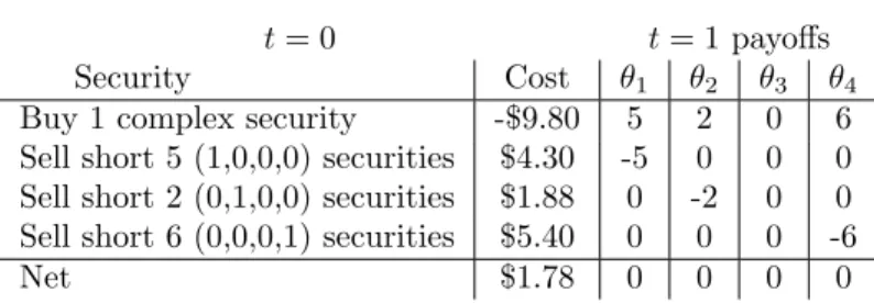
We see that the complex security is relatively undervalued vis-a-vis the state claim prices. This suggests acquiring a positive amount of the complex secu-rity while selling (short) the replicating portfolio of state claims. Table 10.1 illustrates a possible combination.
the same good should be identical. If this were not the case, a riskless and costless arbitrage opportunity would open up: Buy extremely large amounts at the low price and sell them at the high price, forcing the two prices to converge. When applied across two different geographical locations, (which is not the case here: our world is a point in space), the law of one price may not hold because of transport costs rendering the arbitrage costly.
Table 10.1: An arbitrage Portfolio
t= 0 t= 1 payoffs
Security Cost θ1 θ2 θ3 θ4
Buy 1 complex security -$9.80 5 2 0 6 Sell short 5 (1,0,0,0) securities $4.30 -5 0 0 0 Sell short 2 (0,1,0,0) securities $1.88 0 -2 0 0 Sell short 6 (0,0,0,1) securities $5.40 0 0 0 -6
Net $1.78 0 0 0 0
So the arbitrageur walks away with $1.78 while (1) having made no invest-ment of his own wealth and (2) without incurring any future obligation (per-fectly hedged). She will thus replicate this portfolio as much as she can. But the added demand for the complex security will, ceteris paribus, tend to increase its price while the short sales of the state claims will depress their prices. This will continue (arbitrage opportunities exist) so long as the pricing relationships are not in perfect alignment.
Suppose now that only complex securities are traded and that there areM
of them (N states). The following is true.
Proposition 10.2: IfM =N, and all theM complex securities are linearly independent, then (i) it is possible to infer the prices of the Arrow-Debreu state-contingent claims from the complex securities’ prices and (ii) markets are effectively complete.2
The hypothesis of linear independence can be interpreted as a requirement that there exist N truly different securities for completeness to be achieved. Thus it is easy to understand that if among theN complex securities available, one security, A, pays (1, 2, 3) in the three relevant states of nature, and the other,B, pays (2, 4, 6), onlyN-1 truly distinct securities are available: Bdoes not permit any different redistribution of purchasing power across states than
A permits. More generally, the linear independence hypothesis requires that no one complex security can be replicated as a portfolio of some of the other complex securities. You will remember that we made the same hypothesis at the beginning of Section 6.3.
Suppose the following securities are traded:
(3,2,0) (1,1,1) (2,0,2)
at equilibrium prices $1.00, $0.60, and $0.80, respectively. It is easy to verify that these three securities are linearly independent. We can then construct the Arrow-Debreu prices as follows. Consider, for example, the security (1,0,0):
(1,0,0) =w1(3,2,0) +w2(1,1,1) +w3(2,0,2)
2When we use the language “linearly dependent,” we are implicitly regarding securities as
Thus, 1 = 3w1+w2+ 2w3
0 = 2w1+w2
0 = w2+ 2w3
Solve: w1= 1/3, w2=−2/3,w3= 1/3,andq(1,0,0)= 1/3(1.00)+(−2/3)(.60)+
1/3(.80) =.1966
Similarly, we could replicate (0,1,0) and (0,0,1) with portfolios (w1 = 0, w2 = 1, w3 = −1/2) and (w1 = −1/3, w2 = 2/3, w3 = 1/6), respectively, and price them accordingly.
Expressed in a more general way, the reasoning just completed amounts to searching for a solution of the following system of equations:
3 1 22 1 0 0 1 2 w 1 1 w12 w13 w1 2 w22 w23 w1 3 w32 w33 = 1 0 00 1 0 0 0 1
Of course, this system has solution
3 1 22 1 0 0 1 2 −1 1 0 00 1 0 0 0 1
only if the matrix
of security payoffs can be inverted, which requires that it be of full rank, or that its determinant be nonzero, or that all its lines or columns be linearly independent.
Now suppose the number of linearly independent securities is strictly less than the number of states (such as in the final, no-trade, example of Section 8.3 where we assume only a risk-free asset is available). Then the securities markets are fundamentally incomplete: There may be some assets that cannot be accurately priced. Furthermore, risk sharing opportunities are less than if the securities markets were complete and, in general, social welfare is lower than what it would be under complete markets: some gains from exchange cannot be exploited due to the lack of instruments permitting these exchanges to take place.
We conclude this section by revisiting the project valuation problem. How should we, in the light of the Arrow-Debreu pricing approach, value an uncertain cash flow stream such as:
t= 0 1 2 3 ... T
−I0 CF˜ 1 CF˜ 2 CF˜ 3 ... CF˜ T
This cash flow stream is akin to a complex security since it pays in multiple states of the world. Let us specifically assume that there areN states at each datet,t= 1, ..., T and let us denoteqt,θthe price of the Arrow-Debreu security
promising delivery of one unit of the numeraire if state θ is realized at date
in the same occurrence. Then pricing the complex security `a la Arrow-Debreu means valuing the project as in Equation (10.1).
N P V =−I0+ T X t=1 N X θ=1 qt,θCFt,θ. (10.1)
Although this is a demanding procedure, it is a pricing approach that is fully general and involves no approximation. For this reason it constitutes an ex-tremely useful reference.
In a risk-free setting, the concept of state contingent claim has a very familiar real-world counterpart. In fact, the notion of the term structure is simply a reflection of “date-contingent” claims prices. We pursue this idea in the next section.
10.3
Constructing State Contingent Claims Prices in a
Risk-Free World: Deriving the Term Structure
Suppose we are considering risk-free investments and risk-free securities exclu-sively. In this setting – where we ignore risk – the “states of nature” that we have been speaking of simply correspond to future time periods. This sec-tion shows that the process of computing the term structure from the prices of coupon bonds is akin to recovering Arrow-Debreu prices from the prices of complex securities.
Under this interpretation, the Arrow-Debreu state contingent claims corre-spond to risk-free discount bonds of various maturities, as seen in Table 10.2.
Table 10.2: Risk-Free Discount Bonds As Arrow-Debreu Securities
Current Bond Price Future Cash Flows
t= 0 1 2 3 4 ... T
−q1 $1,000
−q2 $1,000
...
−qT $1,000
where the cash flow of a “j-period discount bond” is just
t= 0 1 ... j j+ 1 ... T
−qj 0 0 $1,000 0 0 0
These are Arrow-Debreu securities because they pay off in one state (the period of maturity), and zero for all other time periods (states).
In the United States at least, securities of this type are not issued for ma-turities longer than one year. Rather, only interest bearing or coupon bonds are issued for longer maturities. These are complex securities by our definition: They pay off in many states of nature. But we know that if we have enough
distinct complex securities we can compute the prices of the Arrow-Debreu se-curities even if they are not explicitly traded. So we can also compute the prices of these zero coupon or discount bonds from the prices of the coupon or interest-bearing bonds, assuming no arbitrage opportunities in the bond market. For example, suppose we wanted to price a 5-year discount bond coming due in November of 2009 (we view t= 0 as November 2004), and that we observe two coupon bonds being traded that mature at the same time:
(i) 77
8% bond priced at 1092532, or $1097.8125/$1,000 of face value
(ii) 55
8% bond priced at 100329, or $1002.8125/$1,000 of face value
The coupons of these bonds are respectively,
.07875∗$1,000 = $78.75 / year
.05625∗$1,000 = $56.25/year3
The cash flows of these two bonds are seen in Table 10.3.
Table 10.3: Present And Future Cash Flows For Two Coupon Bonds
Bond Type Cash Flow at Time t
t= 0 1 2 3 4 5
77/8 bond: −1,097.8125 78.75 78.75 78.75 78.75 1,078.75
55/8 bond: −1,002.8125 56.25 56.25 56.25 56.25 1,056.25
Note that we want somehow to eliminate the interest payments (to get a discount bond) and that 78.75
56.25 = 1.4 So, consider the following strategy: Sell
one 77/8% bond while simultaneously buying 1.4 unit of 55/8% bonds. The
corresponding cash flows are found in Table 10.4.
Table 10.4 : Eliminating Intermediate Payments
Bond Cash Flow at Timet
t= 0 1 2 3 4 5
−1x 77/8 bond: +1,097.8125 −78.75 −78.75 −78.75 −78.75 −1,078.75
+1.4x 55/8 bond: −1,403.9375 78.75 78.75 78.75 78.75 1,478.75
Difference: −306.125 0 0 0 0 400.00
The net cash flow associated with this strategy thus indicates that thet= 0 price of a $400 payment in 5 years is $306.25. This price is implicit in the pricing of our two original coupon bonds. Consequently, the price of $1,000 in 5 years must be
$306.125×1000
400 = $765.3125
3In fact interest is paid every 6 months on this sort of bond, a refinement that would double
Alternatively, the price today of $1.00 in 5 years is $.7653125. In the notation of our earlier discussion we have the following securities:
θ1 θ2 θ3 θ4 θ5 78.75 78.75 78.75 78.75 1078.75 and 56.25 56.25 56.25 56.25 1056.25 and we consider −4001 78.75 78.75 78.75 78.75 1078.75 + 1.4400 56.25 56.25 56.25 56.25 1056.25 = 0 0 0 0 1 .
This is an Arrow-Debreu security in the riskless context we are considering in this section.
If there are enough coupon bonds with different maturities with pairs coming due at the same time and with different coupons, we can thus construct a complete set of Arrow-Debreu securities and their implicit prices. Notice that the payoff patterns of the two bonds are fundamentally different: They are linearly independent of one another. This is a requirement, as per our earlier discussion, for being able to use them to construct a fundamentally new payoff pattern, in this case, the discount bond.
Implicit in every discount bond price is a well defined rate of return notion. In the case of the prior illustration, for example, the implied 5-year compound risk free rate is given by
$765.3125(1 +r5)5 = $1000, or r5 = .078
This observation suggests an intimate relationship between discounting and Arrow-Debreu date pricing. Just as a full set of date claims prices should allow us to price any risk free cash flow, the rates of return implicit in the Arrow-Debreu prices must allow us to obtain the same price by discounting at the equivalent family of rates. This family of rates is referred to as term structure of interest rates.
Definition: The term structure of interest rates r1, r2, ... is the family of interest rates corresponding to risk free discount bonds of successively greater maturity; i.e.,ri is the rate of return on a risk free discount bond maturing i
periods from the present.
We can systematically recover the term structure from coupon bond prices provided we know the prices of coupon bonds of all different maturities. To
illustrate, suppose we observe risk-free government bonds of 1,2,3,4-year matu-rities all selling at par4with coupons, respectively, of 6%, 6.5%,7.2%, and 9.5%.
We can construct the term structure as follows:
r1: Since the 1-year bond sells at par, we haver1= 6%;
r2: By definition, we know that the two year bond is priced such that 1000 = 65
(1 +r1)+ 1065
(1 +r2)2 which, given thatr1= 6%,solves forr2= 6.5113%. r3: is derived accordingly as the solution to
1000 = 72 (1 +r1)+ 72 (1 +r2)2 + 1072 (1 +r3)3
Withr1 = 6% and r2 = 6.5113%, the solution is r3= 7.2644%. Finally, given these values forr1 tor3, r4 solves:
1000 = 95 (1 +r1)+ 95 (1 +r2)2+ 95 (1 +r3)3 + 1095 (1 +r4)4, i.e.,r4= 9.935%.
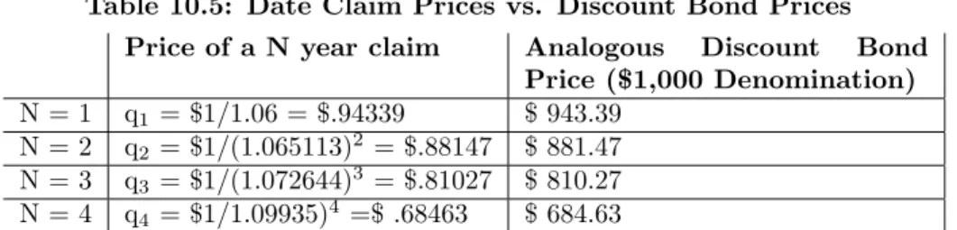
Note that these rates are the counterpart to the date contingent claim prices. Table 10.5: Date Claim Prices vs. Discount Bond Prices
Price of a N year claim Analogous Discount Bond Price ($1,000 Denomination) N = 1 q1= $1/1.06 = $.94339 $ 943.39
N = 2 q2= $1/(1.065113)2 = $.88147 $ 881.47
N = 3 q3= $1/(1.072644)3 = $.81027 $ 810.27
N = 4 q4= $1/1.09935)4 =$ .68463 $ 684.63
Of course, once we have the discount bond prices (the prices of the Arrow-Debreu claims) we can clearly price all other risk-free securities; for example, suppose we wished to price a 4-year 8% bond:
t= 0 1 2 3 4
−p0(?) 80 80 80 1080
and suppose also that we had available the discount bonds corresponding to Table 10.5 as in Table 10.6.
Then the portfolio of discount bonds (Arrow-Debreu claims) which replicates the 8% bond cash flow is (Table 10.7):
{.08 x 1-yr bond, .08 x 2-yr bond, .08 x 3-yr bond, 1.08 x 4-yr bond}. 4That is, selling at their issuing or face value, typically of $1,000.
Table 10.6: Discount Bonds as Arrow-Debreu Claims
Bond Price (t=0) CF Pattern
t= 1 2 3 4
1-yr discount -$943.39 $1,000
2-yr discount -$881.47 $1,000
3-yr discount -$810.27 $1,000
4-yr discount -$684.63 $1,000
Table 10.7: Replicating the Discount Bond Cash Flow
Bond Price (t=0) CF Pattern
t= 1 2 3 4
08 1-yr discount (.08)(−943.39) =−$75.47 $80(80 state 1 A-D claims)
08 2-yr discount (.08)(−881.47) =−$70.52 $80(80 state 2 A-D claims) 08 3-yr discount (.08)(−810.27) =−$64.82 $80 1.08 4-yr discount (1.08)(−684.63) =−$739.40 $1,080 Thus: p4yr.8% bond =.08($943.39) +.08($881.47) + 08($810.27) + 1.08($684.63) = $950.21.
Notice that we are emphasizing, in effect, the equivalence of the term struc-ture of interest rates with the prices of date contingent claims. Each defines the other. This is especially apparent in Table 10.5.
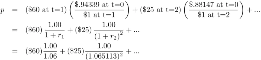
Let us now extend the above discussion to consider the evaluation of arbi-trary risk-free cash flows: any such cash flow can be evaluated as a portfolio of Arrow-Debreu securities; for example:
t= 0 1 2 3 4
60 25 150 300
We want to price this cash flow today (t= 0) using the Arrow-Debreu prices we have calculated in Table 10.4.
p = ($60 at t=1) µ $.94339 at t=0 $1 at t=1 ¶ + ($25 at t=2) µ $.88147 at t=0 $1 at t=2 ¶ +... = ($60) 1.00 1 +r1 + ($25) 1.00 (1 +r2)2 +... = ($60)1.00 1.06+ ($25) 1.00 (1.065113)2 +...
The second equality underlines the fact thatevaluating risk-free projects as portfolios of Arrow-Debreu state contingent securities is equivalent to
discount-ing at the term structure: = 60 (1 +r1) + 25 (1 +r2)2+ 150 (1 +r3)3 +...etc
In effect, we treat a risk-free project as a risk-free coupon bond with (potentially) differing coupons. There is an analogous notion of forward prices and its more familiar counterpart, the forward rate. We discuss this extension in Appendix 10.1.
10.4
The Value Additivity Theorem
In this section we present an important result illustrating the power of the Arrow-Debreu pricing apparatus to generate one of the main lessons of the CAPM. Let there be two assets (complex securities)aandbwith date 1 payoffs ˜
zaand ˜zb, respectively, and let their equilibrium prices bepa and pb. Suppose
a third asset, c, turns out to be a linear combination ofa and b. By that we mean that the payoff toccan be replicated by a portfolio ofaandb. One can thus write
˜
zc =Az˜a+Bz˜b,for some constant coefficientsAandB (10.2)
Then the proposition known as the Value Additivity Theorem asserts that the same linear relationship must hold for the date 0 prices of the three assets:
pc=Apa+Bpb.
Let us first prove this result and then discuss its implications. The proof easily follows from our discussion in Section 10.2 on the pricing of complex securities in a complete market Arrow-Debreu world. Indeed, for our 2 securities
a,b, one must have:
pi=
X
s
qszsi,i=a, b (10.3)
where qs is the price of an Arrow-Debreu security that pays one unit of
con-sumption in states(and zero otherwise) andzsiis the payoff of asset iin state
s
But then, the pricing ofcmust respect the following relationships:
pc= X s qszsc= X s qs(Azsa+Bzsb) = X s (Aqszsa+Bqszsb) =Apa+Bpb
The first equality follows from the fact thatcis itself a complex security and can thus be priced using Arrow-Debreu prices [i.e., an equation such as Equation (10.3) applies]; the second directly follows from Equation (10.2); the third is a pure algebraic expansion that is feasible because our pricing relationships are fundamentally linear; and the fourth follows from Equation (10.3) again.
Now this is easy enough. Why is it interesting? Think of aandb as being two stocks with negatively correlated returns; we know that c, a portfolio of these two stocks, is much less risky than either one of them. Butpc is a linear
combination ofpa and pb. Thus, the fact that they can be combined in a less
risky portfolio has implications for the pricing of the two independently riskier securities and their equilibrium returns. Specifically, it cannot be the case that
pc would behigh because it corresponds to a desirable, riskless, claim while the
pa andpb would below because they are risky.
To see this more clearly, let us take an extreme example. Suppose that a
and b are perfectly negatively correlated. For an appropriate choice of A and
B, sayA∗ and B∗,the resulting portfolio, call it d, will have zero risk; i.e., it
will pay a constant amount in each and every state of nature. What should the price of this riskless portfolio be? Intuitively, its price must be such that purchasingdatpd will earn the riskless rate of return. But how could the risk
ofaandbbe remunerated while, simultaneously, dwould earn the riskless rate and the value additivity theorem hold? The answer is that this is not possible. Therefore, there cannot be any remuneration for risk in the pricing ofaand b. The pricespa and pb must be such that the expected return on a andb is the
riskless rate. This is true despite the fact thataandbare two risky assets (they do not pay the same amount in each state of nature).
In formal terms, we have just asserted that the two terms of the Value Additivity Theorem ˜zd =A∗z˜a+B∗z˜b and pd =A∗pa+B∗pb, together with
the fact thatdis risk-free,
Ez˜d pd = 1 +rf, force Ez˜a pa = E˜zb pb = 1 +rf.
What we have obtained in this very general context is a confirmation of one of the main results of the CAPM: Diversifiable risk is not priced. If risky assets a and b can be combined in a riskless portfolio, that is, if their risk can be diversified away, their return cannot exceed the risk-free return. Note that we have made no assumption here on utility functions nor on the return expectations held by agents. On the other hand we have explicitly assumed that markets are complete and that consequently each and every complex security can be priced (by arbitrage) as a portfolio of Arrow-Debreu securities.
It thus behooves us to describe how Arrow-Debreu state claim prices might actually be obtained in practice. This is the subject of the remaining sections to Chapter 10.
10.5
Using Options to Complete the Market: An Abstract
Setting
Let us assume a finite number of possible future date-states indexedi= 1,2, ..., N. Suppose, for a start, that three states of the world are possible in dateT = 1,
yet only one security (a stock) is traded. The single security’s payoffs are as follows: State Payoff θ1 θ2 θ3 12 3 .
Clearly this unique asset is not equivalent to a complete set of state-contingent claims. Note that we can identify the payoffs with the ex-post price of the security in each of the 3 states: the security pays 2 units of the numeraire commodity in state 2 and we decide that its price then is $2.00. This amounts to normalizing the ex post, date 1, price of the commodity to $1, much as we have done at date 0. On that basis, we can consider call options written on this asset with exercise prices $1 and $2, respectively. These securities are contracts giving the right (but not the obligation) to purchase the underlying security at prices $1 and $2, respectively, tomorrow. They are contingent securities in the sense that the right they entail is valuable only if the price of the underlying security exceeds the exercise price at expiration, and they are valueless otherwise. We think of the option expiring at T = 1, that is, when the state of nature is revealed.5 Thestates of naturestructure enables us to be specific regarding what
these contracts effectively promise to pay. Take the call option with exercise price $1. If state 1 is realized, that option is a right to buy at $1 the underlying security whose value is exactly $1. The option is said to beat the money and, in this case, the right in question is valueless. If state 2 is realized, however, the stock is worth $2. The right to buy, at a price of $1, something one can immediately resell for $2 naturally has a market value of $1. In this case, the option is said to bein the money. In other words, atT = 1, when the state of nature is revealed, an option is worth the difference between the value of the underlying asset and its exercise price, if this difference is positive, and zero otherwise. The complete payoff vectors of these options at expiration are as follows: CT([1,2,3] ; 1) = 01 2 θ1θ2 θ3 at the money in the money in the money . Similarly, CT([1,2,3] ; 2) = 00 1 θ1θ2 θ3
5In our simple two-date world there is no difference between an American option, which
can be exercised at any date before the expiration date, and a European option, which can be exercised only at expiration.
In our notation,CT(S;K) is the payoff to a call option written on security
S with exercise price K at expiration date T. We useCt(S;K) to denote the
option’s market price at timet≤T . We frequently drop the time subscript to simplify notation when there is no ambiguity.
It remains now to convince ourselves that the three traded assets (the un-derlying stock and the two call options, each denoted by its payoff vector at
T) θ1 θ2 θ3 12 3 , 01 2 , 00 1
constitute a complete set of securities markets for states (θ1,θ2,θ3). This is so because we can use them to create all the state claims. Clearly
00 1 is present. To create 01 0 , observe that 01 0 =w1 12 3 +w2 01 2 +w3 00 1 , wherew1= 0, w2= 1,andw3=−2. The vector 10 0
can be similarly created.
We have thus illustrated one of the main ideas of this chapter, and we need to discuss how general and applicable it is in more realistic settings. A preliminary issue is why trading call option securitiesC([1,2,3];1) andC([1,2,3];2) might be the preferred approach to completing the market, relative to the alternative possibility of directly issuing the Arrow-Debreu securities [1,0,0] and [0,1,0]? In the simplified world of our example, in the absence of transactions costs, there is, of course, no advantage to creating the options markets. In the real world, however, if a new security is to be issued, its issuance must be accompanied by costly disclosure as to its characteristics; in our parlance, the issuer must disclose as much as possible about the security’s payoff in the various states. As there may be no agreement as to what the relevant future states are – let alone what the payoffs will be – this disclosure is difficult. And if there is no consensus as to its payoff pattern, (i.e., its basic structure of payoffs), investors will not want to hold it, and it will not trade. But the payoff pattern of an option on an already-traded asset is obvious and verifiable to everyone. For this reason, it is, in principle, a much less expensive new security to issue. Another way to describe the advantage of options is to observe that it is useful conceptually, but difficult in practice, to define and identify a single state of nature. It is more practical to define contracts contingent on a well-definedrange of states. The fact that these states are themselves defined in terms of, or revealed via, market prices is another facet of the superiority of this type of contract.
Note that options are by definition in zero net supply, that is, in this context
X
k
Ctk([1,2,3] ;K) = 0
whereCk
t ([1,2,3] ;K) is the value of call options with exercise price K, held by
agent k at time t ≤ T. This means that there must exist a group of agents with negative positions serving as the counter-party to the subset of agents with positive holdings. We naturally interpret those agents as agents who have written the call options.
We have illustrated the property that markets can be completed using call options. Now let us explore the generality of this result. Can call options always be used to complete the market in this way? The answer is not necessarily. It depends on the payoff to the underlying fundamental assets. Consider the asset:
θ1 θ2 θ3 22 3 .
For any exercise priceK, all options written on this security must have payoffs of the form: C([2,2,3] ;K) = 22−−KK 3−K 00 3−K ifK≤ 2 if 2< K ≤3 Clearly, for anyK,
22 3 and 22−−KK 3−K
have identical payoffs in stateθ1andθ2, and, therefore, they cannot be used to generate Arrow-Debreu securities
10 0 and 01 0 .
There is no way to complete the markets with options in the case of this underlying asset. This illustrates the following truth: We cannot generally write options that distinguish between two states if the underlying assets pay identical returns in those states.
The problem just illustrated can sometimes be solved if we permit options to be written onportfolios of the basic underlying assets. Consider the case of
four possible states atT = 1, and suppose that the only assets currently traded are θ1 θ2 θ3 θ4 1 1 2 2 and 1 2 1 2 .
It can be shown that it is not possible, using call options, to generate a com-plete set of securities markets using only these underlying securities. Consider, however, the portfolio composed of 2 units of the first asset and 1 unit of the second: 2 1 1 2 2 + 1 1 2 1 2 = 3 4 5 6 .
The portfolio pays a different return in each state of nature. Options written on the portfolio alone can thus be used to construct a complete set of traded Arrow-Debreu securities. The example illustrates a second general truth, which we will enumerate as Proposition 10.3.
Proposition 10.3: A necessary as well as sufficient condition for the cre-ation of a complete set of Arrow-Debreu securities is that there exists a single portfolio with the property that options can be written on it and such that its payoff pattern distinguishes among all states of nature.
Going back to our last example, it is easy to see that the created portfolio and the three natural calls to be written on it:
3 4 5 6 plus 0 1 2 3 (K=3) and 0 0 1 2 (K=4) and 0 0 0 1 (K=5)
are sufficient, (i.e., constitute a complete set of markets in our four-state world). Combinations of the (K = 5) and (K = 4) vectors can create:
0 0 1 0 .
Combinations of this vector, and the (K = 5) and (K = 3) vectors can then create: 0 1 0 0 , etc.
Probing further we may inquire ifthe writing of callson the underlying assets is always sufficient, or whether there are circumstances under which other types of options may be necessary. Again, suppose there are four states of nature, and consider the following set ofprimitive securities:
θ1 θ2 θ3 θ4 0 0 0 1 1 1 0 1 0 1 1 1 .
Because these assets pay either one or zero in each state, calls written on them will either replicate the asset itself, or give the zero payoff vector. The writing of call options will not help because they cannot further discriminate among states. But suppose we write a put option on the first asset with exercise price 1. A put is a contract giving the right, but not the obligation, tosell an underlying security at a pre-specified exercise price on a given expiration date. The put option with exercise price 1 has positive value atT = 1 in those states where the underlying security has value less than 1. The put on the first asset with exercise price = $1 thus has the following payoff:
1 1 1 0 =PT([0,0,0,1] ; 1).
You can confirm that the securities plus the put are sufficient to allow us to construct (as portfolios of them) a complete set of Arrow-Debreu securities for the indicated four states. In general, one can prove Proposition 10.4.
Proposition 10.4:
If it is possible to create, using options, a complete set of traded securities, simple put and call options written on the underlying assets are sufficient to accomplish this goal.
That is, portfolios of options are not required.
10.6
Synthesizing State-Contingent Claims: A First
Ap-proximation
The abstract setting of the discussion above aimed at conveying the message that options are natural instruments for completing the markets. In this section, we show how we can directly create a set of state-contingent claims, as well as their equilibrium prices, using option prices or option pricing formulae in a more realistic setting. The interest in doing so is, of course, to exploit the possibility, inherent in Arrow-Debreu prices, of pricing any complex security. In
this section we first approach the problem under the hypothesis that the price of the underlying security or portfolio can take only discrete values.
Assume that a risky asset is traded with current price S and future price
ST. It is assumed that ST discriminates across all states of nature so that
Proposition 10.3 applies; without loss of generality, we may assume that ST
takes the following set of values:
S1< S2< ... < Sθ< ... < SN,
where Sθ is the price of this complex security if state θ is realized at date T.
Assume also that call options are written on this asset with all possible exercise prices, and that these options are traded. Let us also assume thatSθ=Sθ−1+δ
for every stateθ. (This is not so unreasonable as stocks, say, are traded at prices that can differ only in multiples of a minimum price change).6 Throughout the
discussion we will fix the time to expiration and will not denote it notationally. Consider, for any state ˆθ, the following portfolioP:
Buy one call withK=Sˆθ−1
Sell two calls withK=Sˆθ
Buy one call withK=Sˆθ+1
At any point in time, the value of this portfolio,VP, is
VP =C
¡
S, K=Sˆθ−1¢−2C¡S, K=Sθˆ
¢
+C¡S, K=Sˆθ+1¢.
To see what this portfolio represents, let us examine its payoffat expiration(refer to Figure 10.1):
Insert Figure 10.1 about here
For ST ≤ Sˆθ−1, the value of our options portfolio, P, is zero. A similar
situation exists for ST ≥Sˆθ+1since the loss on the 2 written calls with K = Sˆθ exactly offsets the gains on the other two calls. In state ˆθ, the value of the portfolio isδ corresponding to the value of CT
¡
Sˆθ, K =Sˆθ−1¢, the other two options being out of the money when the underlying security takes value Sˆθ. The payoff from such a portfolio thus equals:
Payoff toP= 0 if ST < Sˆθ δ if ST =Sˆθ 0 if ST > Sˆθ
in other words, it pays a positive amountδ in state ˆθ, and nothing otherwise. That is, it replicates the payoff of the Arrow-Debreu security associated with state ˆθup to a factor (in the sense that it paysδ instead of 1). Consequently, 6Until recently, the minimum price change was equal to $1/16 on the NYSE. At the end
of 2000,decimal pricing was introduced whereby the prices are quoted to the nearest $1/100 (1 cent).
the current price of the state ˆθ contingent claim (i.e., one that pays $1.00 if state ˆθ is realized and nothing otherwise) must be
qˆθ=1
δ
£
C¡S, K=Sˆθ−1¢+C¡S, K=Sˆθ+1¢−2C¡S, K=Sˆθ¢¤.
Even if these calls are not traded, if we identify our relevant states with the prices of some security – say the market portfolio – then we can use readily available option pricing formulas (such as the famous Black & Scholes formula) to obtain the necessary call prices and, from them, compute the price of the state-contingent claim. We explore this idea further in the next section.
10.7
Recovering Arrow-Debreu Prices From Options Prices:
A Generalization
By the CAPM, the only relevant risk is systematic risk. We may interpret this to mean that the only states of nature that are economically or financially relevant are those that can be identified with different values of the market portfolio.7
The market portfolio thus may be selected to be the complex security on which we write options, portfolios of which will be used to replicate state-contingent payoffs. The conditions of Proposition 10.1 are satisfied, guaranteeing the pos-sibility of completing the market structure.
In Section 10.6, we considered the case for which the underlying asset as-sumed a discrete set of values. If the underlying asset is the market portfolioM, however, this cannot be strictly valid: As an index it can essentially assume an infinite number of possible values. How is this added feature accommodated?
1. Suppose that ST, the price of the underlying portfolio (we may think of
it as a proxy forM), assumes acontinuum of possible values. We want to price an Arrow-Debreu security that pays $1.00 if ˜ST ∈
h
−δ
2+ ˆST,SˆT+δ2
i
, in other words, ifST assumes any value in a range of width δ, centered on ˆST. We are
thus identifying our states of nature with ranges of possible values for the market portfolio. Here the subscriptT refers to the future date at which the Arrow-Debreu security pays $1.00 if the relevant state is realized.
2. Let us construct the following portfolio8 for some small positive number ε >0,
Buy one call withK= ˆST −δ2−ε
Sell one call withK= ˆST−δ2
Sell one call withK= ˆST+δ2
Buy one call withK= ˆST +δ2+ε.
7That is, diversifiable risks have zero market value (see Chapter 7 and Section 10.4). At
an individual level, personal risks are, of course, also relevant. They can, however, be insured or diversified away. Insurance contracts are often the most appropriate to cover these risks. Recall our discussion of this issue in Chapter 1.
8The option position corresponding to this portfolio is known as abutterfly spread in the
Figure 10.2 depicts what this portfolio paysat expiration. Insert Figure 10.2 about here
Observe that our portfolio pays εon a range of states and 0 almost every-where else. By purchasing 1/ε units of the portfolio, we will mimic the payoff of an Arrow-Debreu security, except for the two small diagonal sections of the payoff line where the portfolio pays something between 0 andε. This undesir-able feature (since our objective is to replicate an Arrow-Debreu security) will be taken care of by using a standard mathematical trick involving taking limits.
3. Let us thus consider buying1/
εunits of the portfolio. The total payment,
when ˆST −δ2 ≤ST ≤SˆT +δ2, isε·1ε ≡1, for any choice ofε. We want to let
ε7→0, so as to eliminate payments in the rangesST ∈
h ˆ ST −2δ −ε,SˆT −δ2 ´ and ST ∈ ³ ˆ ST+δ2,SˆT+δ2+ε i . The value of1/
ε units of this portfolio is:
1 ε n C(S, K= ˆST − δ 2 −ε)−C(S, K= ˆST − δ 2) −£C(S, K= ˆST +δ 2)−C(S, K= ˆST + δ 2+ε) ¤o , where a minus sign indicates that the call was sold (thereby reducing the cost of the portfolio by its sale price). On balance the portfolio will have a positive price as it represents a claim on a positive cash flow in certain states of nature. Let us assume that the pricing function for a call with respect to changes in the exercise price can be differentiated (this property is true, in particular, in the case of the Black & Scholes option pricing formula). We then have:
lim ε7→0 1 ε n C(S, K= ˆST −δ 2−ε)−C(S, K= ˆST− δ 2) −£C(S, K= ˆST +δ 2)−C(S, K= ˆST + δ 2+ε) ¤o = −lim ε7→0 C ³ S, K= ˆST −δ2−ε ´ −C ³ S, K= ˆST −δ2 ´ −ε | {z } ≤0 +lim ε7→0 C ³ S, K= ˆST +δ2+ε ´ −C ³ S, K= ˆST +δ2 ´ ε | {z } ≤0 = C2 µ S, K= ˆST +δ 2 ¶ −C2 µ S, K= ˆST −δ 2 ¶ .
Here the subscript 2 indicates the partial derivative with respect to the second argument (K), evaluated at the indicated exercise prices. In summary, the limiting portfolio has a payoff at expiration as represented in Figure 10.3
Insert Figure 10.3 about here and a (current) price C2
³ S, K= ˆST +δ2 ´ −C2 ³ S, K= ˆST−δ2 ´ that is posi-tive since the payoff is posiposi-tive. We have thus priced an Arrow-Debreu state-contingent claim one period ahead, given that we define states of the world as coincident with ranges of a proxy for the market portfolio.
4. Suppose, for example, we have an uncertain payment with the following payoff at timeT: CFT = ½ 0 if ST ∈/[ ˆST −δ2,SˆT +δ2] 50000 if ST∈[ ˆST −2δ,SˆT +δ2] ¾ .
The value today of this cash flow is: 50,000· · C2 µ S, K= ˆST+δ 2 ¶ −C2 µ S, K= ˆST −δ 2 ¶¸ .
The formula we have developed is really very general. In particular, for any arbitrary valuesS1
T andST2, the price of an Arrow-Debreu contingent claim that
pays off $1.00 if the underlying market portfolio assumes a valueST ∈
£ S1 T, ST2 ¤ , is given by q¡ST1, ST2 ¢ =C2¡S, K=ST2 ¢ −C2¡S, K=ST1 ¢ . (10.4)
We value this quantity in Box 10.1 for a particular set of parameters making explicit use of the Black-Scholes option pricing formula.
Box 10.1: Pricing A-D Securities with Black-Scholes
For calls priced according to the Black-Scholes option pricing formula, Bree-den and Litzenberger (1978) prove that
AD¡ST1, ST2 ¢ = C2¡S, K=ST2 ¢ −C2¡S, K=ST1 ¢ = e−rT©N¡d2¡S1 T ¢¢ −N¡d2¡S2 T ¢¢ª where d2(Si T) = h ln³S0 Si T ´ +³rf −δ−σ 2 2 ´ Ti σ√T
In this expression,T is the time to expiration,rf the annualized continuously
compounded riskless rate over that period,δthe continuous annualized portfolio dividend yield,σthe standard deviation of the continuously compounded rate of return on the underlying index portfolio,N( ) the standard normal distribution, andS0 the current value of the index.
Suppose the continuously-compounded risk-free rate is .06, the not-continuously compounded dividend yield isδ = .02, T = 5 years,S0 = 1,500,
S2 T = 1,700,ST1 = 1,600,σ= .20; then d2(S1 T) = n ln¡ 1500 1600 ¢ +hln(1.06)−ln(1.02)−(.20)2 2i (.5)o .20√.5 = {−.0645 + (.0583−.0198−.02)(.5)} .1414 = −.391 d2(S2 T) = © ln¡1500 1700 ¢ + (.0583−.0198−.02)(.5)ª .1414 = {−.1252 +.00925)} .1414 = −.820 AD(S1T, ST2) = e−ln(1.06)(.5){N(−.391)−N(−.820)} = .9713{.2939−.1517} = .1381, or about $.14. ¤
Suppose we wished to price an uncertain cash flow to be received in one period from now, where a period corresponds to a duration of timeT. What do we do? Choose several ranges of the value of the market portfolio corresponding to the various states of nature that may occur – say three states: “recession,” “slow growth,” and “boom” and estimate the cash flow in each of these states (see Figure 10.4). It would be unusual to have a large number of states as the requirement of having to estimate the cash flows in each of those states is likely to exceed our forecasting abilities.
Insert Figure 10.4 about here
Suppose the cash flow estimates are, respectively,CFB, CFSG, CFR, where
the subscripts denote, respectively, “boom,” “slow growth,” and “recession.” Then, Value of theCF =VCF =q ¡ S3 T, ST4 ¢ CFB+q ¡ S2 T, ST3 ¢ CFSG+q ¡ S1 T, ST2 ¢ CFR, where S1
T < ST2 < ST3 < ST4, and the Arrow-Debreu prices are estimated
from option prices or option pricing formulas according to Equation (10.4). We can go one (final) step further if we assume for a moment that the cash flow we wish to value can be described by a continuous function of the value of the market portfolio.
In principle, for a very fine partition of the range of possible values of the market portfolio, say{S1, ..., SN}, whereSi< Si+1,SN = maxST,andS1= min
ST, we could price the Arrow-Debreu securities that pay off in each of theseN−1
states defined by the partition:
q(S1, S2) = C2(S, S2)−C2(S, S1)
q(S2, S3) = C2(S, S3)−C2(S, S2) ,..etc.
Simultaneously, we could approximate a cash flow function CF(ST) by a
function that is constant in each of these ranges ofST (a so-called “step
func-tion”), in other words, ˆCF(ST) =CFi,forSi−1≤ST ≤Si. For example,
ˆ
CF(ST) =CFi= CF(S, ST =Si) +CF(S, ST =Si−1)
2 forSi−1≤ST ≤Si This particular approximation is represented in Figure 10.5. The value of the approximate cash flow would then be
VCF = N X i=1 ˆ CFi·q(Si−1,Si) = N X i=1 ˆ CFi[C2(S, ST =Si)−C2(S, ST =Si−1)] (10.5)
Insert Figure 10.5 about here
Our approach is now clear. The precise value of the uncertain cash flow will be the sum of the approximate cash flows evaluated at the Arrow-Debreu prices as the norm of the partition (the size of the intervalSi−Si−1) tends to zero. It
can be shown (and it is intuitively plausible) that the limit of Equation (10.5) as max
i |Si+1−Si| 7→ 0 is the integral of the cash flow function multiplied by
the second derivative of the call’s price with respect to the exercise price. The latter is the infinitesimal counterpart to the difference in the first derivatives of the call prices entering in Equation (10.4).
lim max i |Si+1−Si|7→0 N X i=1 ˆ CFi[C2(S, ST =Si+1)−C2(S, ST =Si)] (10.6) = Z CF(ST)C22(S, ST)dST.
As a particular case of a constant cash flow stream, a risk-free bond paying $1.00 in every state is then priced as per
prf = 1 (1 +rf)= ∞ Z 0 C22(S, ST)dST.
Box 10.2: Extracting Arrow-Debreu Prices from Option Prices: A Numerical Illustration
Let us now illustrate the power of the approach adopted in this and the previ-ous section. For that purpose, Table 10.8 [adapted from Pirkner, Weigend, and Zimmermann (1999)] starts by recording call prices, obtained from the Black-Scholes formula for a call option, on an underlying index portfolio, currently valued at S = 10 , for a range of strike prices going from K = 7 to K = 13 (columns 1 and 2). Column 3 computes the value of portfolio P of Section 10.6. Given that the difference between the exercise prices is always 1 (i.e.,δ= 1), holding exactly one unit of this portfolio replicates the $1.00 payoff of the Arrow-Debreu security associated withK = 10. This is shown on the bottom line of column 7, which corresponds toS = 10. From column 3, we learn that the price of this Arrow-Debreu security, which must be equal to the value of the replicating portfolio, is $0.184. Finally, the last two columns approximate the first and second derivatives of the call price with respect to the exercise price. In the current context this is naturally done by computing the first and second differences (the price increments and the increments of the increments as the exercise price varies) from the price data given in column 2. This is a literal application of Equation (10.4). One thus obtains the full series of Arrow-Debreu prices for states of nature identified with values of the underlying market port-folios ranging from 8 to 12, confirming that the $0.184 price occurs when the state of nature is identified asS = 10 (or 9.5< S <10.5).
Table 10.8: Pricing an Arrow-Debreu State Claim Cost of Payoff if ST = K C(S, K) Position 7 8 9 10 11 12 13 ∆C ∆(∆C) =qθ 7 3.354 -0.895 8 2.459 0.106 -0.789 9 1.670 +1.670 0 0 0 1 2 3 4 0.164 -0.625 10 1.045 -2.090 0 0 0 0 -2 -4 -6 0.184 -0.441 11 0.604 +0.604 0 0 0 0 0 1 2 0.162 -0.279 12 0.325 0.118 -0.161 13 0.164 0.184 0 0 0 1 0 0 0
10.8
Arrow-Debreu Pricing in a Multiperiod Setting
The fact that the Arrow-Debreu pricing approach is static makes it most ad-equate for the pricing of one-period cash flows and it is, quite naturally, in this context that most of our discussion has been framed. But as we have em-phasized previously, it is formally equally appropriate for pricing multiperiod cash flows. The estimation (for instance via option pricing formulas and the methodology introduced in the last two sections) of Arrow-Debreu prices for several periods ahead is inherently more difficult, however, and relies on more perilous assumptions than in the case of one period ahead prices. (This parallels the fact that the assumptions necessary to develop closed form option pricing formulae are more questionable when they are used in the context of pricing long-term options). Pricing long-term assets, whatever the approach adopted, requires making hypotheses to the effect that the recent past tells us something about the future, which, in ways to be defined and which vary from one model to the next, translates into hypotheses that some form of stationarity prevails. Completing the Arrow-Debreu pricing approach with an additional stationarity hypothesis provides an interesting perspective on the pricing of multiperiod cash flows. This is the purpose of the present section.
For notational simplicity, let us first assume that the same two states of nature (ranges of value ofM) can be realized in each period, and that all future state-contingent cash flows have been estimated. The structure of the cash flow is found in Figure 10.6.
Insert Figure 10.6
Suppose also that we have estimated, using our formulae derived earlier, the values of the one-period state-contingent claims as follows:
Tomorrow 1 2 Today 12 · .54 .42 .46 .53 ¸ =q
where q11 (= .54) is the price today of an Arrow-Debreu claim paying $1 if state 1 (a boom) occurs tomorrow, given that we are in state 1 (boom) today. Similarly, q12 is the price today of an Arrow-Debreu claim paying $1 if state 2 (recession) occurs tomorrow given that we are in state 1 today. Note that these prices differ because the distribution of the value of M tomorrow differs depending on the state today.
Now let us introduce our stationarity hypothesis. Suppose thatq, the matrix of values, is invariant through time.9 That is, the same two states of nature
describe the possible futures at all future dates and the contingent one-period prices remain the same. This allows us to interpret powers of theqmatrix,q2,
q3, . . . in a particularly useful way. Considerq2(see also Figure 10.7):
q2= · .54 .42 .46 .53 ¸ · · .54 .42 .46 .53 ¸ = · (.54) (.54) + (.42) (.46) (.54) (.42) + (.42) (.53) (.46) (.54) + (.53) (.46) (.46) (.42) + (.53) (.53) ¸
Note there are two ways to be in state 1 two periods from now, given we are in state 1 today. Therefore, the price today of $1.00, if state 1 occurs in two periods, given we are in state 1 today is:
(.54)(.54)
| {z }
value of $1 in 2 periods if state 1 occurs and the intermediate state is 1
+ (.42)(.46)
| {z }
value of $1.00 in 2 periods if state 1 occurs and the intermediate state is 2
.
Similarly,q2
22= (.46)(.42) + (.53)(.53) is the price today, if today’s state is 2, of
$1.00 contingent on state 2 occurring in 2 periods. In general, for powersN of the matrixq, we have the following interpretation forqN
ij: Given that we are in
stateitoday, it gives the price today of $1.00, contingent on statej occurring in
N periods. Of course, if we hypothesized three states, then the Arrow-Debreu matrices would be 3×3 and so forth.
How can this information be used in a “capital budgeting” problem? First we must estimate the cash flows. Suppose they are as outlined in Table 10.9.
Table 10.9: State Contingent Cash Flows
t= 0 1 2 3 state 1 state 2 · 42 65 ¸ · 48 73 ¸ · 60 58 ¸
Then the present value (P V) of the cash flows, contingent on state 1 or state
to compute forward Arrow-Debreu prices; in other words, the Arrow-Debreu matrix would change from date to date and it would have to be time-indexed. Mathematically, the procedure described would carry over, but the information requirement would, of course, be substantially larger.
2 are given by: P V = · P V1 P V2 ¸ = · .54 .42 .46 .53 ¸ · 42 65 ¸ + · .54 .42 .46 .53 ¸2· 48 73 ¸ + · .54 .42 .46 .53 ¸3· 60 58 ¸ = · .54 .42 .46 .53 ¸ · 42 65 ¸ + · .4848 .4494 .4922 .4741 ¸ · 48 73 ¸ + · .4685 .4418 .4839 .4580 ¸ + · 60 54 ¸ = · 49.98 53.77 ¸ + · 56.07 58.23 ¸ + · 53.74 55.59 ¸ = · 159.79 167.59 ¸ .
This procedure can be expanded to include as many states of nature as one may wish to define. This amounts to choosing as fine a partition of the range of possible values ofM that one wishes to choose. It makes no sense to construct a finer partition, however, if we have no real basis for estimating different cash flows in those states. For most practical problems, three or four states are probably sufficient. But an advantage of this method is that it forces one to think carefully about what a project cash flow will be in each state, and what the relevant states, in fact, are.
One may wonder whether this methodology implicitly assumes that the states are equally probable. That is not the case. Although the probabili-ties, which would reflect the likelihood of the value ofM lying in the various intervals, are not explicit, they are built into the prices of the state-contingent claims.
We close this chapter by suggesting a way to tie the approach proposed here with our previous work in this Chapter. Risk-free cash flows are special (degen-erate) examples of risky cash flows. It is thus easy to use the method of this section to price risk-free flows. The comparison with the results obtained with the method of Section 10.3 then provides a useful check of the appropriateness of the assumptions made in the present context.
Consider our earlier example with Arrow-Debreu prices given by: 1 2 State 1 State 2 · .54 .42 .46 .53 ¸
If we are in state 1 today, the price of $1.00 in each state tomorrow (i.e., a risk-free cash flow tomorrow of $1.00) is .54 + 42 = .96. This implies a risk-free rate of: ¡ 1 +r1 f ¢ =1.00 .96 = 1.0416 or 4.16%.
To put it differently, .54 + .42 = .96 is the price of a one-period discount bond paying $1.00 in one period, given that we are in state 1 today. More generally, we would evaluate the following risk-free cash flow as:
t= 0 1 2 3 100 100 100 P V = · P V1 P V2 ¸ = · .54 .42 .46 .53 ¸ · 100 100 ¸ + · .54 .42 .46 .53 ¸2· 100 100 ¸ + · .54 .42 .46 .53 ¸3· 100 100 ¸ = · .54 .42 .46 .53 ¸ · 100 100 ¸ + · .4848 .4494 .4922 .4741 ¸ · 100 100 ¸ + · .4685 .4418 .4839 .4580 ¸ · 100 100 ¸ So P V1 = [.54 +.42]100 + [.4848 +.4494]100 + [.4685 +.4418] = [.96]100 + [.9342]100 + [.9103]100 = 280.45
where [.96] = price of a one-period discount bond given state 1 today, [.9342] = price of a two-period discount bond given state 1 today, [.9103] = price of a three-period discount bond given state 1 today. TheP V given state 2 is computed analogously. Now this provides us with a verification test: If the price of a discount bond using this method does not coincide with the prices using the approach developed in Section 10.3 (which relies on quoted coupon bond prices), then this must mean that our states are not well defined or numerous enough or that the assumptions of the option pricing formulae used to compute Arrow-Debreu prices are inadequate.
10.9
Conclusions
This chapter has served two main purposes. First, it has provided us with a platform to think more in depth about the all-important notion of market completeness. Our demonstration that, in principle, a portfolio of simple calls and puts written on the market portfolio might suffice to reach a complete market structure suggests the ‘Holy Grail’ may not be totally out of reach. Caution must be exercised, however, in interpreting the necessary assumptions. Can we indeed assume that the market portfolio – and what do we mean by the latter – is an adequate reflection of all the economically relevant states of nature? And the time dimension of market completeness should not be forgotten. The most relevant state of nature for a Swiss resident of 40 years of age may be the possibility of a period of prolonged depression with high unemployment in Switzerland 25 years from now (i.e., when he is nearing retirement10). Now
extreme aggregate economic conditions would certainly be reflected in the Swiss Market Index (SMI), but options with 20-year maturities are not customarily 10The predominant pension regime in Switzerland is a defined benefit scheme with the