Warsaw University
Faculty of Mathematics, Informatics and Mechanics
Jacek Sroka
Models and languages for specification of
collection-oriented scientific workflows
PhD dissertation
Supervisors dr hab. Jerzy Tyszkiewicz and dr Jan Hidders Institute of Informatics Warsaw University October 2008
Author’s declaration:
aware of legal responsibility I hereby declare that I have written this disser-tation myself and all the contents of the disserdisser-tation have been obtained by legal means.
October 24, 2008 . . . .
date Jacek Sroka
Supervisor’s declaration:
the dissertation is ready to be reviewed
October 24, 2008 . . . .
date dr hab. Jerzy Tyszkiewicz
October 24, 2008 . . . .
Abstract
In many sciences, like ecology, geology, chemistry, astronomy and especially bioinformatics, structured data is analyzed with the use of collection-oriented scientific workflow (COSW) systems. Such systems allow to describe the experiments with a kind of network, through which the data flows and is processed, and where the nodes of the network carry out domain specific operations.
Many specialized COSW workbenches exist and are based on simple yet expressive graphical notations, integrate most important tools, services and databases from a given domain, and include various additional useful fea-tures like data provenance tracking or service discovery. The models, lan-guages and techniques used in COSW modeling have become an interesting topic of study themselves and are the focus of this thesis. They have many relationships with workflow modeling, business process modeling, databases, computational grids and many more established research areas.
The main contributions of this thesis are: (1) investigation and formal-ization of the semantics of Scufl — the COSW specification language of a popular Taverna workbench, and (2) the creation of a new formal model for specification of COSWs, that combines both the control flow and data manipulation aspects and is as close as possible to the existing models from workflow and database domains allowing to reuse available theoretical results.
Key words
DFL, collection-oriented scientific workflow, workflow systems, Petri net, nested relational calculus
Thematic classification
D. Software
D.3 Programming languages D.3.2 Language classifications
Contents
1 Introduction 1
1.1 Collection-oriented scientific workflows . . . 1
1.2 Existing systems . . . 2
1.2.1 Taverna workbench . . . 3
1.2.2 Kepler . . . 6
1.2.3 BioKleisli . . . 8
1.2.4 Other systems . . . 11
1.3 Problems that will be addressed . . . 11
1.4 Structure of the thesis . . . 12
2 Scufl 13 2.1 Motivation of formal semantics for Scufl . . . 13
2.2 Scufl type system . . . 14
2.3 Scufl global components . . . 17
2.4 Scufl syntax . . . 18
2.4.1 Hierarchically nested Scufl graphs . . . 22
2.5 Processor execution . . . 24
2.5.1 An overview of processor execution . . . 24
2.5.2 Extended complex value construction and deconstruction 26 2.5.3 Incoming-links strategy semantics . . . 27
2.5.4 Product strategy semantics . . . 28
2.6 Transition system semantics . . . 34
2.6.1 Scufl graph state . . . 34
2.6.2 Ready ports and enabled processors . . . 37
2.6.3 Finished Scufl graphs . . . 39
2.6.4 Scufl graph initialization and result collection . . . 41
2.6.5 State transitions . . . 42
2.7 Dealing with heterogeneous values in Taverna . . . 53
2.7.1 Allowing heterogeneous lists . . . 54
2.7.2 Adapting the semantics to avoid heterogeneous lists . . 55
2.8 Related work on Scufl semantics . . . 56
3 DataFlow Language 58 3.1 Motivation . . . 60
3.2 Combining NRC and Petri nets . . . 60
3.2.1 Nested relational calculus . . . 60
3.2.2 Petri nets . . . 61
3.2.3 How we combine NRC and Petri nets . . . 62
3.3 Syntax . . . 64
3.3.1 The type system . . . 65
3.3.2 Edge naming function . . . 66
3.3.3 Transition naming function . . . 66
3.3.4 Edge annotation function . . . 66
3.3.5 Place type function . . . 67
3.3.6 Dataflow . . . 67
3.4 Transition labels . . . 69
3.4.1 Core transition labels . . . 70
3.4.2 Extension transition labels . . . 71
3.5 Transition system semantics . . . 71
3.5.1 Token unnesting history . . . 72
3.5.2 Semantics of transitions . . . 76
3.6 A bioinformatics example . . . 79
3.7 Hierarchical collection-oriented scientific workflows . . . 82
3.7.1 Refinement rules . . . 85
3.7.2 The bioinformatics example revisited . . . 96
3.8 DFL designer . . . 99
3.8.1 Correctness enforcement . . . 101
3.8.2 Enactment optimization . . . 103
3.8.3 Debugging and testing COSWs with interactive firing of transitions . . . 106
3.8.4 Further research . . . 106
4 Summary of the presented results and further research 108 4.1 Summary . . . 108
4.3 Further research . . . 110
A Basic properties of lexicographical ordering of number
Chapter 1
Introduction
1.1
Collection-oriented scientific workflows
Information technology techniques and results developed for business appli-cations are constantly challenged by new needs emerging from dynamically growing applied sciences. This is especially true for the domains of database systems and workflow processing, since even larger volumes of data have to be analyzed and the analysis processes become even more complex. Where those two domains coincide a new interesting field of research on collection-oriented scientific workflows (COSWs) emerges.In many sciences, like ecology, geology, chemistry, astronomy and espe-cially bioinformatics, structured data is analyzed by a software system orga-nized into a kind of network, through which the data flows and is processed, and where the nodes of the network carry out domain specific operations. This is similar to doing workflow processing in business, but here more em-phasis is put on the processing of collections of data values and less on the control flow issues, hence we propose the term collection-oriented scientific workflow (COSW).
The basic operations in such workflows are mainly specialized, domain-specific data analysis algorithms. Their efficient implementations are avail-able as open source tools or are made freely accessible on dedicated Internet servers maintained by scientific institutions. The results produced by the workflows are used to form scientific hypotheses and to justify or invalidate them. The way a COSW is organized, i.e., which operations are executed and how they depend on each others results, is important and is usually
published in some form together with the results of the data processing ex-periment. This is necessary for the reviewers and readers to understand what was done in the experiment, to effectively and objectively assess its merit, to repeat and verify it, and finally to adapt it for their own research projects.
Traditionally such data processing experiments, have been performed by copying and pasting data between local programs, e.g., the components of the EMBOSS package [52], and web accessible processing servers with WWW forms type user interfaces, like FASTA Sequence Comparison at the Univer-sity of Virginia [61] and the Basic Local Alignment Search Tool at NCBI [42]. This method of experimenting is laborious and error prone. It has also been common to construct ad hoc scripts and programs to automatize this task, but for that at least some basic knowledge of programming and distributed programming issues is necessary. Furthermore, the produced software usually has been not portable and poorly, if at all, documented.
Nowadays, specialized scientific workflow workbenches such as Taverna [45, 30] and Kepler [35] are used. They are based on simple yet expressive graph-ical notations, integrate most important tools, services and databases from a given domain, and include various additional useful features like data prove-nance tracking or service discovery. The models, languages and techniques used in COSW modeling have become an interesting topic of study themselves and are the focus of this thesis. They have many relationships with work-flow modeling, business process modeling, databases, computational grids and many more established research areas.
1.2
Existing systems
In this section we list popular existing scientific workflow systems. We also review three that seem to be the most interesting in the context of this the-sis, i.e., widely used Taverna, incorporating multiple models of computation Kepler and BioKleisli which has a strong theoretical background. This choice has been mainly motivated by the interesting design of models and languages for specifying workflows that those systems are based on.
All three systems come from the domain of bioinformatics, which is presently a thriving research area. The application of scientific workflow systems in bioinformatics is a sign of strife to transfer the emphasis of the biology research from wet laboratory to computer laboratory, i.e., to con-duct as large part of the experiments as possible in silico as opposed to
traditionally doing everything in vitro. If accomplished this allows to test quickly and cheaply scientific hypotheses before engaging in time consuming wet laboratory tests, i.e., with the use of test tubes and expensive chemical reagents.
1.2.1
Taverna workbench
Taverna [45, 30] is an easy to operate workbench for COSW development and enactment. It allows users to graphically construct COSWs from libraries of available components and is intended for use in bioinformatics data analysis experiments. The most important virtues of Taverna are that it is very easy to use, has a specialized and expressive graphical specification language and integrates thousands [46] of data analysis tools. It also includes additional useful features like service discovery, storing intermediate results and tracking data provenance. The workbench is being constantly developed, but it is already considered stable and has been used in real life research, e.g., [57, 34]. A small example of a Taverna COSW is given in Fig. 1.1 (a). A set of workflow inputs is indicated by a dotted rectangle with a small triangle pointing upwards, which in this case contains one input labeled pin. The graph also contains a set of workflow outputs indicated by a dotted rectan-gle with a small trianrectan-gle pointing downwards, here containing two outputs labeled ppout and pout. Furthermore, the graph contains several so-called processors which represent operations from the Taverna services and which are labeled “Get Nucleotide FASTA”, “Merge String list to string”, “emma”, “showalign” and “prettyplot”. For each processor, depending on the view set-tings, the input ports are listed in the top row, as is done here, or in the left column, as in some of the following examples. Similarly, the output ports are listed in the bottom row or in the right column. For example, the processor with label “emma” has one input port labeled sequence data direct and one output port labeled outseq.
The COSW defines a simple yet often needed experiment. If a pin in-put port is initiated with a list of nucleotide sequence identifiers, then the “Get Nucleotide FASTA” processor implicitly iterates on this list and with the use of an external service that searches the GenBank database [6] returns FASTA formatted nucleotide sequences that correspond to the identifiers. The next processor merges the list of those sequences into one long string, on which the “emma” processor, which is a wrapper for the ClustalW opera-tion of the EMBOSS [52] package, performs a sequence alignment. The final
(a)
(c) (b)
two processors, “showalign” and “prettyplot” are used to present the output respectively in a textual and graphical manner.
As can be noticed, the graphical representation of the COSW communi-cates well the main intent of the experiment. In the following examples we introduce other important features of the system and then we proceed with formal definitions and discussions of these features.
The second example is abstract and is presented in Fig. 1.1 (b). The graph has three branches that independently process their own input values. All the computed values, i.e., the results of “foo1”, “foo2” and “foo3” processors, are directed to theoutworkflow output. Although it is not visible in the graphical representation of the COSW, for the outworkflow output an incoming-links strategy is specified. It determines how the value for a port is obtained in case of multiple data edges ending in it. This strategy can be either merge or select-first, where merge waits for values to arrive from all incoming data edges and packs them into a list while select-first selects the first value that arrives and ignores the others. Example use cases for the different incoming-links strategies in this abstract COSW would be:
• for the merge strategy — obtaining nucleotide sequences from a number of databases and packing them together into a list for further process-ing, e.g., alignment,
• for select-first strategy — requesting the same computation with differ-ent services and continuing the processing with the result that arrives the quickest.
An extra feature of the select-first strategy is that the COSW is less error prone. In Taverna processors can fail, for example if no connection can be made with them over the Internet. Here the COSW finishes properly if at least one of the used tools, i.e., “foo1”, “foo2” or “foo3”, finishes with success. The third example is taken from the myExperiment [23] workflow repos-itory. It is presented in Fig. 1.1 (c) and is incorporated as a building block into several COSWs defining real-life in silico experiments that are also published in the repository. First, it shows that in the Taverna COSWs there are two kinds of edges. The data edges, indicated by solid edges with an arrow head, represent data flow by connecting workflow inputs or output ports of processors with input ports of processors or workflow outputs. The control edges indicated by gray edges ending with a circle represent additional control flow. They connect two processors specifying
that one can execute only when the other has successfully finished. Sec-ond, the example presents how a combination of failing processors, con-trol edges and ports with many incoming edges and the select-first strat-egy specified can be used to model conditional behavior. The COSW re-turns a sequence in a FASTA format that corresponds to a sequence or sequence entry identifier provided as an input. If a sequence identifier, in
database:identifier format, e.g. uniprot:wap_rat, is provided as the
in-put, then the “Fail if sequence” processor succeeds but the “Fail if identifier” fails and thus the “fetchData” processor uses the EBI’s WSDbfetch web ser-vice (seehttp://www.ebi.ac.uk/Tools/webservices/services/dbfetch) to retrieve the sequence in FASTA format. Otherwise the “Fail if sequence” processor fails but the “Fail if identifier” succeeds and the sequence is passed through the Soaplab [33, 53] “seqret” service to force it into a FASTA format. Both conditional branches are joined with theSequenceworkflow output for which the select-first strategy is specified.
Taverna includes other interesting features like product strategies and nested COSWs, which are beyond this short presentation. A further and complete discussion of this system is given in Chapter 2.
1.2.2
Kepler
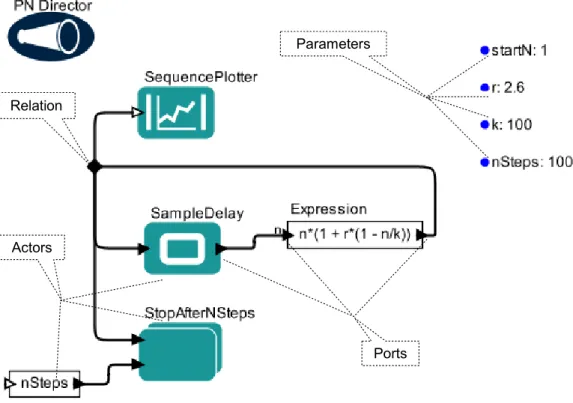
The Kepler scientific workflow system [35] is applied in many areas includ-ing bioinformatics, ecology, oceanography and geology. It is based on the Ptolemy II [17] system, which is a modeling and simulation environment, and extends it with new features and components for COSW design and for efficient workflow execution. Similarly as in Taverna (see 1.2.1) COSWs are specified as graphs where the nodes, here called actors, have input and out-put ports and represent scientific operations. Ports can be connected with channels to define the flow of data. Additional control flow constructs, as loops and branches, are also present and COSWs can be nested with the use ofnested actors. An example COSW with a legend is presented in Figure 1.2. It is an adapted version of an example provided with the Kepler user docu-mentation. It solves a discrete finite-difference equation, that determines a resource-limited population growth, with a growth factor “r”, and a carrying capacity “k”.
A distinguishing feature of Kepler is its ability to enact one and the same COSW according to different computation models which the COSW author specifies with the so calleddirector. Kepler includes directors that correspond
Ports Actors
Relation
Parameters
Figure 1.2: An example of a COSW in Kepler
to process network, synchronous dataflow, continuous time, discrete event, and finite state machine computation models. In our example, both the top level COSW and the nested COSW StopAtEndN, use the process network director. Together with its restriction — the synchronous dataflow director — they are the most frequently used ones. We will characterize the process network model by explaining how the example from Fig. 1.2 works.
The execution in process network model is driven by input data availabil-ity, i.e., an actor can fire, if some input data tokens are available on all its input ports. On the output ports it produces tokens with the result values, which are immediately transfered to further actors. Yet, there are excep-tions. In the example from Fig. 1.2 a special actor SampleDelay is used to start the loop. Without needing any input data tokens on its single input port, it fires once and produces a token with the value assigned to COSW parameter startN. Later on it behaves as an identity operation, which out-puts the value it consumes. The value produced by the SampleDelay actor
is used as the previous population size “n” by the actor that evaluates the formula. Then, three copies of the newly computed population size are made. The first is provided to the SequencePlotter actor that updates a diagram with the computed results. The second is provided to the SampleDelay ac-tor to continue the loop. Finally, the third is provided to a nested COSW StopAfterNSteps, which contains a Counter actor that has an internal state and counts the number of times it is executed. When that value reaches the parameter nSteps, which is endlessly provided to the nested COSW by a Constant actor nSteps, the StopAfterNSteps nested COSW uses another actor it contains, namely Stop actor, to finish the computation. If a Stop actor was not used explicitly, then the COSW would continue indefinitely since the nSteps constant actor would not stop producing tokens and the loop would continue.
In Kepler polymorphic COSWs can be defined, as discussed in [37]. The definition of polymorphic COSWs is based on a technique that is similar to that of the implicit iteration in Taverna, where an actor that expects input of a certain type can also operate on collections of other types by automatically identifying nested values of the right type and operating on them. This type of polymorphic actor is referred to by the authors of [37] as collection-aware actors. A difference with Taverna is that the user can specify in more detail how such nested values are identified and how they are iterated over, where in Taverna this is completely transparent. Another difference with Taverna is that Kepler features an elaborate and refined type system which explicitly allows heterogeneous values and this type system is used in the specification of the aforementioned collection-aware actors.
Thanks to the inclusion of different computational models that can be combined in one COSW, the availability of loops and the presence of special actors like theCounter actor, which has an internal state, or theSampleDelay actor, which does not need input tokens to fire for the first time, Kepler is very expressive as compared to other COSW systems. By expressive we mean here that difficult problems can be solved in Kepler with COSWs of small size. The trade off is that Kepler COSWs are hard to analyze with formal methods and difficult to understand by users with small programming experience.
1.2.3
BioKleisli
BioKleisli [14] is a system allowing querying and transforming complex data from heterogeneous sources, including ones available through a network,
which was developed for and used in the Human Genome Project [62]. It is not a COSW system per se. It provides neither graphical notation nor deals with control flow issues, but is very interesting because of the way how complex collections of data can be processed and because of its theoretical background. It is based on a query language called Collection Program-ing Language (CPL) [71], which is amenable to optimizations and which on nested relational data has the expressive power of nested relational alge-bra [70]. The design of CPL is based on nested relational calculus (NRC) [9] (see 3.2.1) — a calculus version of the nested relational algebra, which is a well studied formalism for querying nested data collections and for which many optimization results are available. It is worth pointing out that in separate research [21, 22] we also studied the usefulness of NRC for COSW specification and analysis. NRC and CPL follow a new approach to query languages inspired by structural recursion [58] and the category theory no-tion of a monad [68, 39]. They are also type orthogonal [14], which means that the design of the language is structured around its type system.
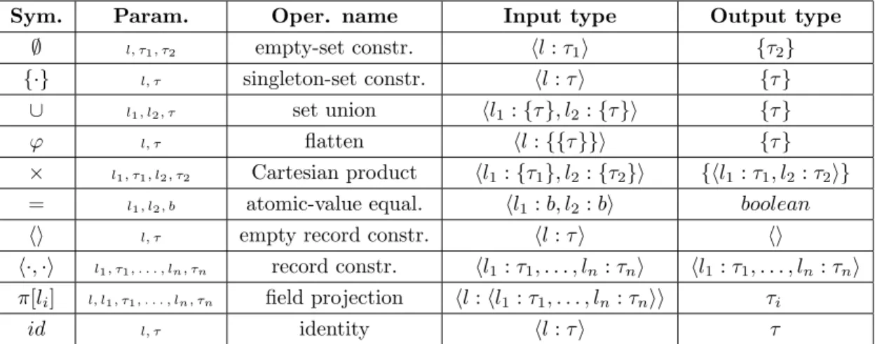
The type system of CPL is given by:
τ ::= bool|int|string |. . .| {τ} | {|τ|} | {||τ||} |
[l1 :τ1, . . . , ln:τn]| hl1 :τ1, . . . , ln :τni
where bool, int, string, . . ., are the base types, {τ}, {|τ|} and {||τ||} are re-spectively set, bag and list types from the typeτ, and [l1 :τ1, . . . , ln :τn] and hl1 :τ1, . . . , ln:τni are respectively record and variant record types with
ele-ment types τ1, . . . , τnand field labels l1, . . . , ln. The semantics of those types
is defined as usual.
The operations of CPL are based on NRC yet the syntax follows Wadler’s work [68] in order to make it more user friendly. CPL is also more robust, for example it is equipped with pattern matching and allows for function definition within the language. We will not give here a complete definition, but limit ourselves to a few simple queries on a database containing a set of COSW system descriptions of type:
Systems ={[name:string, domains:{string}, authors:{string}]}
An example fragment of data conforming to this type is: DB ={[name= “BioKleisli”,
domains={“bioinformatics”},
authors={“S. Davidson”,“C. Overton”,“V. Tannen”,“L. Wong”}
], . . .}
In the query:
{[name=s.name, domains=s.domains]| \s <−DB}
on the right-hand side of | the variable\s traverses the set DB. The result set is constructed on the left-hand side of | by projecting the records to fields name and domains. In the case of bag construction the duplicates would be kept and for lists the order of traversal would be maintained.
In the next query:
{[domains=d]|[name= “BioKleisli”, domains=\d, . . .]<−DB}
only the records with name = “BioKleisli” contribute to the result. As we can see the ellipsis “. . . ” can be used to match the remaining record fields.
A normalization of the data on names and domains can be achieved with the query:
{[name=n, domain=d]
|[name=\n, domains=\dd, . . .]<−DB,\d <−dd}
which results in a set of string pairs with a COSW system name and one of its domains. Note, that this and the next query would not be possible in the flat relational calculus.
Finally, the query:
{[domain=d, names ={x.name| \x <−DB, d <−x.domains}]
| \y <−DB,\d <−y.domains}
restructures the records so that for each domain a set of COSW system names is stored as opposed to a set of domains for each COSW system name.
1.2.4
Other systems
Some other COSW systems include:
• DiscoveryNet [54] — from the domains of bioinformatics and chemistry;
• Triana [36] — from the domain of astronomy;
• Pegasus [15] — from the domains of astronomy and bioinformatics;
• SCIRun [32] — general usage, applied in biomedicine and bioelectric field modeling;
• JOpera [48] — general usage web service composition tool, applied in bioinformatics.
The newest systems can be tracked with help of on-line survey sites as [55, 24], that are maintained by the scientific community. Also business workflow tools can be used to define and enact scientific workflows, yet they are usually control flow oriented, i.e., lack the ability to manipulate complex collections of data, and an additional work is required to integrate services from scientific domains.
1.3
Problems that will be addressed
We start with studying and formalizing the semantics of the process model of the Taverna workbench, which is one of the most popular COSW systems used in bioinformatics. Our goal is to precisely and comprehensively describe all its features, especially those that distinguish it from other workflow sys-tems, examine their usefulness and discuss alternatives. Although we strive for an elegant formal model, we make only a minimal number of compro-mises in order to describe the current Taverna implementation as faithfully as possible. This way when later a clean core model of Taverna is devised it is possible to asses its fidelity.
Because the formalization of Taverna turns out to be very involved, the question rises whether it is possible to design a simpler language with an easier to understand formal semantics that can describe COSWs. For this purpose we investigate if and how existing results on databases and classical workflow modeling can be applied in the COSW research. There exist simple,
clean and well studied formal models of workflows which deal only with con-trol flow and ignore processing of nested collections of data, e.g., Petri nets (see 3.2.2). Similarly, simple, clean and well studied formal models exist for dealing with nested collections of data, but ignore the specification of control flow, e.g., NRC (see 3.2.1). In the remainder of the thesis we are concerned with the creation of a new hybrid formal model for specification of COSWs from first principles, that combines both the control flow and data manipula-tion aspects. Our aim is to structure the new model as close as possible to the existing models from both domains, such that the reuse of results available for them is possible. We also study if and how such a hybrid formal model can be useful in practice, i.e., in real life scientific workflow experiments. For that we construct a new COSW system and test it on real-life experiments adapted from Taverna workbench.
1.4
Structure of the thesis
In Chapter 2 we have investigated and formalized the semantics of Scufl — the COSW specification language of Taverna workbench. Then we use the semantics to prove some basic properties of all COSWs defined in Scufl.
In Chapter 3 we formally define DFL (as in DataFlow Language) — a new language for specifying COSWs which is a combination of Petri nets and NRC. In Section 3.7 we present that certain results for its components can also be applied for DFL. Then, in Section 3.8, we present a tool that allows one to design, enact and analyze DFL COSWs.
Finally, in Chapter 4, we summarize our results and indicate interesting areas and problems for further research that are motivated by the results covered in this thesis.
Chapter 2
Scufl
In this chapter we investigate and formalize the semantics of Scufl, study its distinguishing features, examine their usefulness and discuss alternatives. The formal definitions which we give not only allow to precisely understand what is really being done in a given experiment. They are also the first step toward automatic correctness verification and allow the creation of auxiliary tools that would detect potential errors and suggest possible solutions to COSW creators, the same way as Integrated Development Environments aid modern programmers. The creation of formal semantics is also essential for work on enactment optimization and in designing the means to effectively query COSW repositories.
2.1
Motivation of formal semantics for Scufl
Scufl includes high level features and mechanisms, like implicit iteration, that make the construction of real life COSWs simpler and allow the programmer to focus on the problem being solved. At the same time the COSWs look less complex and can be used in research papers to convey the main idea of anin silicoexperiment that was conducted. Yet, distributed data-processing experiments are complex in nature and a highly expressive definition language that hides much of the complexity of the COSW behind implicit semantics is not the silver bullet. When problems appear, e.g., while debugging, it is important to exactly understand what computation is being done. And even when the specification of the COSW is successfully finished, it’s merit has to be effectively and objectively assessed by reviewers. For this a precise andformal semantics is needed.
It’s also obvious that thein silico experiments that are being conducted become more and more complex and sooner or later automatic verification procedures, similar to those used for verifying complex business transactions, will have to be developed. For such verification the existence of formal se-mantics is a necessary first step as well as for the creation of auxiliary tools that would detect potential errors and suggest possible solutions to COSW creators, the same way as Integrated Development Environments aid modern programmers.
Another domain for which a formal semantics is fundamental is enactment optimization. As with database queries the programmer could only specify what has to be done and the determination of the most effective execution strategy would be left to the COSW engine. In addition, with COSWs being applied more and more frequently, and being shared in Internet reposito-ries [23], their querying is becoming an interesting scientific problem [10, 5]. A successful COSW query language should take into account the semantics and not just the syntax, i.e., compare what the COSWs do and not only how they are defined.
Finally, we argue that the very act of formulating a formal semantics is useful because it forces us to do a complete and thorough analysis of the behavior of Taverna. The formulation of an elegant and natural formal se-mantics is a good litmus test for checking if the current behavior is consistent and well chosen. Such a test is not unimportant for large, complex and rela-tively rapidly evolving systems such as Taverna. In addition, as is shown in this thesis later on, it may provide inspiration for other interesting alterna-tive semantics. Therefore the formulation of a formal semantics can help in the future design and development of Taverna.
2.2
Scufl type system
As the Taverna authors notice “the problem of data typing in life sciences is simply too hard to attack”. There is only one basic type that describes binary data with an attached MIME annotation and we will denote this basic type as M. The MIME annotation is used to determine how a basic type data value is going to be presented to the user, e.g., whether a text, a picture, or its binary representation is going to be displayed. The set of MIME values is denoted asVM. For our examples we will usually assume it contains at least
the natural numbers and strings.
In Taverna we meet in practice only one collection type, namely, ordered lists, even though the documentation suggests that Scufl was designed to support other collection types such as partial orders, trees, bags and sets. Although the user documentation mentions only homogeneous lists, the work-bench does not prevent the use of heterogeneous lists, i.e., lists containing elements of different types such as [1,[2],3,[[4]]]. Heterogeneous lists can be obtained from homogeneous ones during the computation. For example, it is possible to specify in a Taverna COSW that an input is computed from different outputs of different processors by combining them into a single list. Therefore we define the set of complex values such that it includes heteroge-neous lists.
The set of complex values, denoted as Vtav, is defined as the smallest set
such that (1) VM⊆ Vtav and (2) ifx1, . . . , xn ∈ Vtav, then the list [x1, . . . , xn]
is in Vtav. The values of these list types will be denoted as [1,2,3] and [[1,2],[3,4],5], the empty list is denoted as [], and the concatenation of lists is denoted with +, so [1,2] + [1,5] + [] = [1,2,1,5]. Note, that this notion of complex value does not include tuples or records.
Although heterogeneous lists can appear in Taverna, they usually cause processors to fail and otherwise are not always processed coherently, e.g., applying the flatten operation to the list [[x],[[y]]], where x and y are some basic values, results in [[x],[y]] while flattening of [[[x]],[y]] results in [[x], y]. It is however quite possible to give an intuitive semantics for Scufl that allows heterogeneous values everywhere and deals with them consistently. There-fore, we will in the formal part of this chapter, for the sake of simplicity and consistency, assume that heterogeneous values are allowed everywhere. If het-erogeneous values never appear, then the semantics defined in this chapter corresponds to the observed behavior of Taverna.
The consistent behavior for the heterogeneous values is owed to the co-herent generalization of semantics of product strategies expressions (see Sec-tion 2.5.4) and implicit iteraSec-tion mechanism (see SecSec-tion 2.5.2). Despite this we usually limit the presentation to homogeneous values only and discuss in Section 2.7 the strategies for adapting the semantics such that the heteroge-neous values are consistently avoided.
Although Taverna does as little typing as possible it still has a notion of complex type, which is defined by the following syntax:
Examples of such types are M, [M], [[M]],et cetera. The set of all complex types is denoted as Ttav. The semantics of these types are defined with
induction on their syntactic structure such that:
• [[M]] = VM, and
• [[[τ]]] = [[τ]]∪ L([[τ]]) where L(V) denotes the set of finite lists over V. Note, that the given type semantics is more liberal than usual and explicitly allow heterogeneous lists. So not only [[1],[2]] ∈ [[[[M]]]] but also [1,[2]] ∈
[[[[M]]]] since 1 ∈ [[M]] ⇒1 ∈ [[[M]]]. Effectively the type only restricts the maximum nesting depth of the complex values in its semantics.
Further motivation for the liberal list type semantics is given by the fact that if the nesting depth of a certain value is lower than expected there is always an intuitive interpretation of that value as a more deeply nested one, namely by nesting it in singleton lists. For example, if a certain processor expects on a certain input port a list of protein identifiers and it receives a value that is an unnested single protein identifier, then it can interpret this as a singleton list containing this protein. This principle can be applied to every type, i.e., a value of type τ can always be interpreted as a value of type [τ] by assuming it is packed in a singleton list. This is reflected in the type semantics by the fact that [[τ]] ⊆ [[[τ]]]. The idea that types are given a semantics that is related to a coercion mechanism can be found in other work such as [4].
Consistently with the given type semantics and the described type coer-cion we define a subtyping relation, denoted by v, over complex types such thatτ vσiff the nesting depth ofτ is less than or equal to the nesting depth ofσ, i.e., eitherτ =M, orτ = [τ0] andσ = [σ0], whereτ0 vσ0. For example,
M v [M], and [M] v [[[M]]], but [[M]] 6v [M]. Clearly, this notion of subtyping is consistent with the given semantics, i.e., for all complex typesτ and σ it holds thatτ vσ iff [[τ]]⊆[[σ]].
Since there is only one basic type, viz. M, it is not hard to see that v
defines a linear order over the complex types. So we can define a function
max :P(Ttav)→ Ttav, such thatmax(T) is the least common upper bound of
T, i.e., the smallest complex typeσ such that for all typesτ ∈T it holds that τ vσ. This means, for example, that max(∅) = M, max({M,[M]}) = [M], and max({[M],[[[M]]]}) = [[[M]]].
2.3
Scufl global components
Here we list the Scufl components that are common to all COSW. We postu-late a countably infinite setP Lofport labelsthat contains all names that can be given to input and output ports of processors as well as to workflow inputs and outputs. The Taverna workbench comes with a huge library of built-in bioinformatics operations, which are mainly external service intermediaries, i.e., programs that call external services. We call this extensible collection of operations theTaverna servicesand model it by a set of service names called T S which can contain an arbitrary number of names.
The interface of a service is defined by tuple types that give the input type and the output type. These tuple types are defined as partial functions σ : P L → Ttav that map a finite subset dom(σ) ⊆ P L, called the domain
of σ, to complex types. We will denote tuple types {(l1, τ1), . . . ,(ln, τn)} as hl1 :τ1, . . . , ln:τni. The set of all tuple types is denoted as Ttup and the set
of all tuple values asVtup. The semantics of a tuple type σ =hl1 :τ1, . . . , ln:
τni, denoted as [[σ]], is defined as the set all functions t : dom(σ) → Vtav
such that for each li ∈ dom(σ) it holds that t(li) ∈ [[τi]]. Such a function {(l1, x1), . . . ,(ln, xn)}will be denoted ashl1 =x1, . . . , ln =xni. For later use
we define a notation for the projection of a tuple type σ on a set of labels L as σ|L such that σ|L = {(l, τ) ∈ σ | l ∈ L} and its counterpart for tuple values as t|L ={(l, v)∈t|l∈L}.
To define the interface of the Taverna services we postulate the func-tions typei : T S → Ttup and typeo : T S → Ttup that give the input type
and output type, respectively, of each service as a tuple type. In addition we define the functions I : T S → P(P L) and O : T S → P(P L) such that for every service name s ∈ T S I(s) gives the set of input port la-bels and O(s) the set of output port labels, i.e., I(s) = dom(typei(s)) and
O(s) = dom(typeo(s)). For example, the interface for the string
concate-nation operation “Concatenate two strings”∈ T S is defined as follows (we abbreviate “Concatenate two strings” to “c t s”):
I(“c t s”) = {string1, string2}
typei(“c t s”) = hstring1 :M, string2 :M i
O(“c t s”) = {output}
typeo(“c t s”) = houtput:M i
maps a tuple of the input type of the service to one of possibly many tuples of the output type. There are several reasons why the result might not be func-tionally dependent on the input. One of them is that the services can have an internal state which influences its result. Also the service can use ran-domized approximation algorithms, which is often the case in bioinformatics. Finally, the service can be based on a database which is constantly updated. So it seems inappropriate to model services with deterministic functions in the description of Taverna’s semantics. Therefore we associate with each la-bel s∈T S a relationF[s]⊆[[typei(s)]]×[[typeo(s)]] such that for each tuple
t ∈[[typei(s)]] there is at least one tuplet0 ∈[[typeo(s)]] such that (t, t0)∈ F[s].
It should be noted at this point that the current implementation of Taverna does not check if a service call returns a tuple with fields of the correct type, but we chose not to model this in the presented formal semantics.
2.4
Scufl syntax
A brief and informal introduction to Scufl has already been given in Sec-tion 1.2.1. Here we follow with addiSec-tional example and formal definiSec-tions.
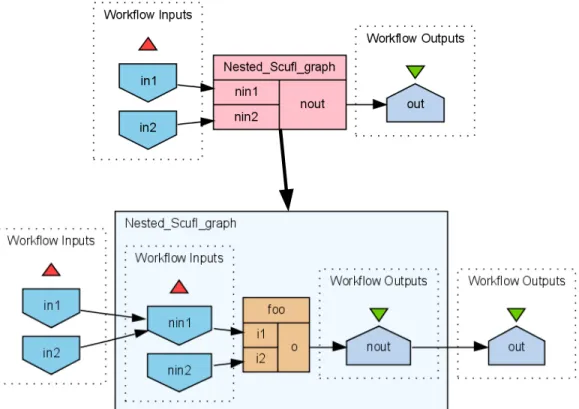
The new example is presented in Fig. 2.1. We start with the analysis of the top Scufl COSW graph which may seem incomplete because thenin2 has no incoming data edges. For that port a default value is specified, but that is not visible in the graphical representation.
Another thing that the diagram does not show are the product strategies associated with all processors. Such strategies are needed because of the implicit iteration semantics of Scufl that was illustrated by the first processor in Fig. 1.1 (a). In general the implicit iteration strategy states that if a processor receives a value that is nested deeper than expected, it will iterate over subvalues of the expected nesting depth and combine the results again in a list. For example, if a processor that computes a function f : [[ha:M i]]→
[[hb :M i]] receives on its port labeled a the value [“foo”,“bar”], then it will compute the list [f(ha= “foo”i), f(ha = “bar”i)]. If a processor computes a function that expects many inputs such asg : [[ha:M, b :M i]]→[[hc:M i]] and is presented with lists of mime values, then a product strategy such as cross product or dot product is required to indicate how the input lists are combined into a single list of tuples that represent the combination of complex values to which the function is applied during the iteration. If the list on port a is [“foo”,“bar”] and the list on port b is [“x”,“y”,“z”] then the
Figure 2.1: An example of a nested Scufl COSW graph
cross product combines them into [[ha = “foo”, b = “x”i,ha = “foo”, b = “y”i,ha = “foo”, b = “z”i],[ha = “bar”, b = “x”i,ha = “bar”, b = “y”i,ha = “bar”, b = “z”i]] and the dot product combines them into [ha = “foo”, b = “x”i,ha = “bar”, b= “y”i]. For an arbitrary number of input ports a product
strategy is defined by an expression in the following syntax: ps ::= ε|P L|(ps⊗ps)|(psps)
in which each label inP Lappears at most once. In this expressionε denotes the empty product strategy, a port label product strategy transforms values into tuples,⊗represents the cross product1andrepresents the dot product.
The set of all product strategies is denoted as P S and the set of port labels used in product strategy ps is denoted as L(ps), i.e., it is defined such that
1For lists the cross product L
1⊗L2 is not equivalent with L2⊗L1 because the order
of the resulting tuples is not the same, but in Taverna there is also a difference in how the result is nested, as will be explained later on.
L(ε) =∅, L(a) = {a} and L(ps1⊗ps2) = L(ps1 ps2) = L(ps1)∪ L(ps2).
The result of a product strategy ps is always a possibly nested list of tuples with fieldsL(ps), e.g., ifps= (a⊗b)c, then this results in a possibly nested list of tuples of the form ha=x, b=y, c=zi.
A product strategy could be relevant for our example if the processor that represents a nested Scufl COSW graph had a merge strategy specified for its nin1 input port, but expected only a single value and not a list. A further explanation of the default value mapping, the incoming-links strategy and the product strategy is provided in Sections 2.5.3 and 2.5.4 respectively.
The final feature presented by the example in Fig. 2.1 is that Scufl COSW graphs are allowed to be recursively nested. The nested Scufl COSW graph is represented by a processor “Nested Scufl graph” and its workflow inputs and outputs match the input ports and output ports of the processor. Nesting a part of a Scufl COSW graph into a processor changes its semantics in two ways. The first is that the nested COSW is not executed until all input ports are ready, and the second is that it will apply the implicit iteration strategy during its execution.
The informal discussion until now was illustrated with a notation that is only one of the ways to represent Scufl COSW graphs and more elaborate representations are available in Taverna, although none of them shows all relevant aspects for understanding the complete semantics of the defined COSW. We follow with a comprehensive formal definition of Scufl COSW graphs — Scufl graphs for short. Since these can be recursively nested it will be an inductive definition. For this definition we postulate a countably infinite set P that contains all possible processor identifiers that we can use in Scufl graphs.
Definition 2.4.1 (Scufl graph). The set of Scufl graphs G is defined as the smallest set such that every Scufl graph composed of Scufl graphs inG is also inG, where such a Scufl graph is defined as a tuple (I, O, P, πi, πo, Ed, Ec, λ, ils,
ps, dv) such that
• I ⊆P L is a finite set of labels representing the workflow inputs,
• O ⊆P L is a finite set of labels representing the workflow outputs,
• P ⊆P is a finite set of processors disjoint withI and O,
• πo ⊆P ×P La finite set representing processor output ports, • Ed⊆(I×πi)∪(πo×πi)∪(πo×O) is a set of data edges, • Ec⊆P ×P is a set of control edges,
• λ:P →(T S∪ G) is the processor labeling function, that maps proces-sors to either a service label in T S or a nested Scufl graph such that for every processor p ∈P it holds that I(λ(p)) = {l | (p, l)∈ πi} and
O(λ(p)) ={l |(p, l)∈πo},
• ils: (πi∪O)→ {first,merge}gives the incoming-links strategy for every
input port of a processor and the workflow outputs,
• ps:P →P Sgives the product strategy for every processor p∈P such that L(ps(p)) ={l |(p, l)∈πi},
• dv :πi → Vtav∪ {⊥} gives a default value2 for each input port, where
⊥ represents the lack of default value and is only allowed if the port has at least one incoming data edge, i.e., if dv((p, l)) = ⊥, then there is a data edge (x,(p, l))∈Ed for some x,
• there are no cycles in the dependency graph which is defined as a directed graph over P such that there is an edge (p1, p2) iff there
is a control edge (p1, p2) ∈ Ec or there is a data edge of the form
((p1, l1),(p2, l2))∈Ed,
where the I andO functions for labels inT S are generalized for Scufl graphs such that for a Scufl graph g we let I(g) and O(g) denote the I and O component of g, respectively.
The restriction that a default value must be specified for input ports that have no arriving data edges is more strict than in the real Taverna 1.7.1, where basic processors are allowed to have input ports with neither an incoming data edge nor a data value. This is an often used feature since basic processors can wrap a service with many optional arguments and flags. However, for the sake of simplicity of presentation we will assume that this is represented in the formal syntax by a basic processor that has exactly the
2In Taverna 1.7.1, the version that was investigated for this thesis, only strings were
set of input ports that are provided and has the semantics that the real basic processor has for that particular set of input ports.
Next to generalizingI we also extend the function typei to Scufl graphs,
i.e., typei : (T S ∪ G) → Ttup. The main purpose of this type is to allow a
processor, that is labeled by λ with a Scufl graph, to determine what type it actually expects, and use that to see if for a given complex value it will do an implicit iteration or pass it on to the nested graph. Recall that if a processor receives a value that is nested deeper than expected, then it will identify the subvalues of the expected nesting depth and iterate over those, i.e., pass them on one by one to the nested Scufl graphs.
Informally, the input type of each workflow input is computed by taking the maximum of the types of processor input ports in the nested Scufl graph to which it is connected. So, for example, if the workflow input is connected to two processor input ports that expect [[M]] and [M], then the Scufl graph is assumed to expect the type [[M]] on this input port. The justification for taking the maximum is that this way the processor that contains the nested Scufl graph only starts implicit iteration if it is really necessary, i.e., none of the nested processors to which the value is passed on can deal with it without iteration. For example, assume that the workflow input is connected to a service with input typehgenes: [M]ithat expects a list of genes encoded as DNA strands and selects the shortest one. Also assume that another service with input typehgen:M iis also connected to this workflow input. Then, if the Scufl graph is given a list of genes, the implicit iteration is only needed for the second service and not the whole Scufl graph. This way the first service can find the shortest gene in the whole input list and not in every singleton list resulting from implicit iteration on the workflow input.
Formally, following the induction of G, the input type of a Scufl graph g = (I, O, P, πi, πo, Ed, Ec, λ, ils, ps, dv) with I = {l1, . . . , ln}, is defined as
typei(g) =hl1 : τ1, . . . , ln : τni, where τi =max({σ(l0)| (li,(p, l0))∈ Ed, σ =
typei(λ(p))}). Note, that this is well defined since the domain of typei(λ(p))
isI(λ(p)), which by the definition of Scufl graph is equal to{l0 |(p, l0)∈πi}.
2.4.1
Hierarchically nested Scufl graphs
The Scufl graph definition is an inductive definition that builds larger Scufl graphs by using smaller ones as labels of its processors, i.e., as nested Scufl graphs. It allows us to define notions and prove theorems with induction on the structure of a Scufl graph. Over the set of all Scufl graphs G we can
define the nesting graph that indicates which Scufl graph is nested in which Scufl graph as follows.
Definition 2.4.2 (The nesting graph). The nesting graph is the directed edge-labeled graph N = (G, E) where G is the set of nodes and the set of edges E ⊆ G ×P× G is defined such that (g, p, g0) ∈ E iff λ(p) = g0 with λ the labeling function of g and pa processor in g.
It is easy to see that, since G is required in its definition to be minimal, there are no directed cycles in N. The set of subgraphs of a Scufl graph g, denoted asGg, is defined as the set of nodes reachable inN fromg, including
g itself. The nesting graph for a particular Scufl graph g is denoted as Ng
and defined as subgraph of N induced byGg.
It is allowed that the same Scufl graph is reused as a label of more than one processor in a certain Scufl graph definition, either within the same subgraph or in different subgraphs. However, the definition of a state of a Scufl graph can be simplified if such reuse is not allowed and therefore we introduce the notion of hierarchically nested Scufl graphs.
Definition 2.4.3 (Hierarchically nested Scufl graphs). A Scufl graph g is said to be hierarchically nested iff Ng is a tree.
Observe that if g is a hierarchically nested Scufl graph then all Scufl graphs in Gg are also necessarily hierarchically nested.
If a Scufl graph is not hierarchical then it can be made so by replacing each occurrence of a certain Scufl graph with a different but isomorphic Scufl graph. For example, if processors p1 and p2 are both labeled with a Scufl
graph g, i.e., λ1(p1) = λ2(p2), where λ1 and λ2 are the processor labeling
function of the subgraphs in which p1 and p2 appear respectively, then we
redefine λ1 and λ2 such that λ1(p1) = g1 and λ2(p2) = g2, where g1 and
g2 are different but isomorphic copies of g that do not appear as subgraphs
themselves. If we start with a certain Scufl graph and repeat this for every two different processors in subgraphs that are labeled with the same Scufl graph, then we will obtain an equivalent hierarchically nested Scufl graph.
In the remainder of this chapter, where we describe the semantics of Scufl graphs, we will do this only for hierarchically nested Scufl graphs, and there-fore, when we refer to a Scufl graph, we always mean a hierarchically nested Scufl graph. The semantics of other Scufl graphs is then defined as the se-mantics of the corresponding hierarchically nested Scufl graphs. The reason
for this is that in a hierarchically nested Scufl graph we can describe the total state as a mapping of each Scufl graph that it contains to its particular state. The exponential blow-up that can be caused by making a Scufl graph hierarchical, is in some sense unavoidable, because it is linked to the poten-tially exponential number of Scufl graph instances for which a state has to be described.
2.5
Processor execution
2.5.1
An overview of processor execution
A successful execution of a processor is a complex event best explained by dividing it in several steps. We give here an informal overview of those steps and discuss the first two of them in the rest of this section in further detail by defining the functions that compute them. Then, in Section 2.6, using those functions and additional prerequisites defined in Section 2.5.2, we discuss the execution of a Scufl graph as a whole, look into all the steps together, and explore all possible scenarios including the possibility of processor failure.
We now proceed with the informal description of the steps of a successful execution of a processor:
Computing the values in the input ports
In the first step an input value for each input port is computed from the values that were sent to it through the incoming data edges. This is done by combin-ing these values into a scombin-ingle complex value accordcombin-ing to the incomcombin-ing-links strategy. The select-first strategy simply takes the first value that arrives and ignores the others, and the merge strategy creates a list containing all the arrived values.
Combining the input port values into the processor input value
A processor input value is computed, which is a single tuple that can be processed by the service that the processor represents, or a possibly nested nested list of such tuples. If for every input port of the processor the value computed in the previous step is of the type expected by the processor, i.e., is not overly nested, then the processor input value is a tuple labeled by input port labels and holding the input port values. For example, if the input
ports are labeled a and b and their computed input port values va and vb
are of the expected type, then the processor input value is ha : va, b : vbi.
If any of the values computed in the preceding steps is too deeply nested, then the values of the different input ports must be combined into a single nested value, i.e., a list of tuples over which the processor can iterate. For example, assume that va is a list of mime values andvb is a list of lists, while
the processor expects types M and [M], respectively. The computation of the processor input value can then be thought of as consisting of two steps. First, the values that were computed for the input ports are transformed into values where the subvalues of the type that is expected are identified by packing them in singleton tuples. Continuing the last example, the value for the input port labeled a would be transformed to a list of tuples of type
ha:M iand the value for the input port labeled bwould be transformed to a list of tuples of typehb: [M]i. Second, the product strategy of the processor describes which combinations of the identified tuples are taken and how they are nested in the result. For example, a strategy consisting of a single cross product will combine all tuples in the first value with all tuples in the second, resulting in a doubly nested list of tuples of type ha :M, b: [M]i.
Performing the execution or the iteration
If the value computed in the preceding step is a tuple, the processor is exe-cuted once, producing one result tuple with values for every output port. If the processor input value is a list, it is iterated over by executing the pro-cessor for each tuple in it. The result for each output port contains a list of values from result tuples of subsequent iteration steps that is structured accordingly to the nesting structure of the processor input list. Following the previous example, if the processor has two output ports labeled candd, and is associated with a Taverna service with output type hc: [M], d:M i, then the iteration will produce a list of lists with elements of type [M] for port labeled c, and a list of lists with elements of type Mfor port labeled d.
Copying the computed output port values
When the normal execution or iteration has finished the values computed in the processor output ports are copied to all processor input ports and workflow outputs to which they are connected.
2.5.2
Extended complex value construction and
decon-struction
As explained in the informal description of the semantics of processor execu-tion in Secexecu-tion 2.5.1, we can describe the execuexecu-tion of a processor after the processor input value has been computed as a process that takes a possibly nested list of tuples, iterates over all tuples by executing the processor and while doing so constructs for each output port a value by inserting, at the position of the original tuple, the value that was computed for that output port by the iteration step.
Since Vtup includes tuples, but not lists of tuples, we define an extended
complex value set Vext as the smallest set such that (1) Vtup ⊆ Vext and (2)
if x1, . . . , xn∈ Vext then the list [x1, . . . , xn] is in Vext.
In order to identify the position of tuples and other subvalues in an ex-tended complex value we introduce the notion of subvalue index. By a sub-value of an extended complex value v we mean v itself, any element of v, any element of element of v, and so on, up to the tuples. For example, if v = [[a, b],[c]], where a, b and c are tuples, then all subvalues of v are: v, [a, b], [c],a,b and c.
Definition 2.5.1 (Subvalue index). A subvalue index, or simply index, is a list of positive natural numbers. Such indices are denoted by a list of numbers separated by slashes, e.g., 2/3/8 and 1/1, and the empty list is denoted as . The set of all complex value indices is denoted as I.
The numbers in an index are listed from most significant on the left, to the least significant on the right. Following the last example, the subsequent indexes of the mentioned subvalues of v are: , 1, 2, 1/1, 1/2 and 2/1.
Formally, the subvalue indicated by an index is defined by the function
get:Vext×I →(Vext∪⊥) such thatget(v, ) = v, andget(v, i/α) = get(vi, α)
ifv = [v1, . . . , vn] and 1≤i≤n, andget(v, i/α) =⊥otherwise. For example,
if v = [[a, b],[c]], thenget(v,2/1) = cand get(v,2/2) = ⊥.
We assume that complex value indices are ordered according to the lex-icographical ordering, i.e., the smallest binary relation over I such that for every i, j ∈ N and α, β ∈ I it holds that (1) α, (2) if i ≤ j, then i/α j/β and (3) if α β, then i/α i/β. As usual this defines a linear order over I.
In order to be able to iterate over all tuples in an extended complex value we define a function that retrieves the index of the first tuple and a function to
jump to the index of the next tuple. The first function isfirst :Vext→(I ∪⊥)
which is defined such thatfirst(v) =αwhereαis the smallest index such that
get(v, α) ∈ Vtup, and first(v) =⊥ if there is no such α. The second function
isnext:Vext× I → (I ∪ ⊥) and is defined such thatnext(v, α) =β if β is the
smallest index larger than α such that get(v, β) ∈ Vtup, and next(v, α) = ⊥
if such a β does not exist.
Finally, we define a function put(v, α, w) that inserts into the complex value v at position α the complex value w, which can be used to construct complex values. For example, put([x,[y]],2/1, z) = [x,[z]] and put([], , z) = z. If the position α does not yet exist in v then it is extended minimally with empty lists to create it. For example, put([],1/1/1, x) = [[[x]]] and
put([],2/1, x) = [[],[x]]. Formally, this function put :Vtav× I × Vtav → Vtav
is defined such that (1) put(v, , w) = w, (2) put(v, i/α, w) = put([], i/α, w) if v ∈ VM, (3) put([],1/α, w) = [put([], α, w)], (4) put([v] + v0,1/α, w) =
[put(v, α, w)] +v0, (5) put([], i/α, w) = [[]] +put([],(i−1)/α, w) if i > 1, (6)
put([v] +v0, i/α, w) = [v] +put(v0,(i−1)/α, w) if i >1.
2.5.3
Incoming-links strategy semantics
Here we define the semantics of incoming-links strategy expressions which are used to indicate how to compute the value for a processor input port or workflow output by composing it from values provided from multiple incom-ing data edges. The computation is done incrementally, that is, a temporary result is extended each time a new value arrives from one of the data edges that did not already supply a value. The lack of a previous temporary value at the start of the process is represented by ⊥.
The select-first incoming-links strategy picks the first value to arrive and ignores all the other. This is the default behavior of processor input ports and workflow outputs. The function [[first]] : ((Vtav∪ {⊥})× Vtav) → Vtav
takes as the first argument the current temporary result and as the second the value provided by the next data edge. As a result the new temporary result is returned. Formally:
[[first]](t, v) =
(
v if t=⊥
t otherwise
The merge incoming-links strategy combines all incoming values as ele-ments of a list. It was added to Taverna 1.3.1 to prevent the need for creation
of user defined n-argument processors that compose their arguments into a list. As with select-first, the merge function [[merge]] : ((Vtav\[[M]]∪ {⊥})×
Vtav) → Vtav has two arguments, yet now the temporary value is never of
type Msince it is a list of values provided so far. Formally: [[merge]](t, v) =
(
[v] if t =⊥
t+ [v] otherwise
Strictly speaking this is not a merge, but we adhere to the Taverna termi-nology.
2.5.4
Product strategy semantics
Here we define the semantics of product strategy expressions ps∈P S. The product strategy expressions are used to transform values from Vtav, that
are provided on individual input ports of a given processor p, to extended complex values that contain tuples of type typei(λ(p)), i.e., lists of tuples
ready to be iterated upon by p.
The values provided on a processors’ input ports have to be combined into a processor input value that is either a single tuple which can be processed by the service that the processor represents or a nested list of such tuples. This is done in two steps. The first step transforms each of the values provided on every input port into a single unary tuple or a list of unary tuples. The tuples’ field is labeled with the same label as the respective input port and they contain values of the type that is expected on that port. The second step combines such preprocessed values for processors with multiple input ports into a single n-ary tuple or a nested list of those.
We now describe the first step in more detail. Its purpose is to identify the subvalues that are of a nesting depth acceptable by the processor. For example, if the value on the input port with label a is [[1,2],[],[3]] and the processor expects a value of type [M] on it, then the value is transformed to [ha = [1,2]i,ha = []i,ha = [3]i]. If this is the only input port, then the processor will iterate over the three values [1,2], [] and [3]. If, on the other hand, value of type Mis expected, then it is transformed to [[ha= 1i,ha= 2i],[],[ha = 3i]] and the processor will iterate over the three values 1, 2 and 3. This is formalized by the packing function packl:τ :Vtav → Vext that
Formally, it is defined as follows:
packl:τ(x) =
(
hl=xi if x∈[[τ]]
[packl:τ(x1), . . . ,packl:τ(xn)] if x= [x1, . . . , xn]6∈[[τ]]
This function is well defined for every x ∈ Vtav, which can be shown with induction on the structure ofx and using the fact thatVM ⊆[[τ]] for any τ ∈ Ttav. It is possible that a value of typeτ contains a nested value that is also
of type τ. For example, if τ = [[M]] and x= [[[1]]], then there are in xthree nested values of type τ, namely 1, [1] and [[1]]. In that case the nested value with the largest nesting depth is chosen and so packa:τ(x) = [ha = [[1]]i]. For a more elaborate example consider:
packa:[M]([[1],[[2],3],4])
= [packa:[M]([1]),packa:[M]([[2],3]),packa:[M](4)] = [ha= [1]i,[packa:[M]([2]),packa:[M](3)],ha= 4i]
= [ha= [1]i,[ha= [2]i,ha = 3i],ha= 4i] Note, that the values 3 and 4 are in [[[M]]] and therefore also packed in a tuple.
We now proceed to the second step where we deal with the case of proces-sors with multiple input ports. There the extended complex values computed by the packing function have to be combined. For this the cross and dot prod-uct strategy expressions are used to represent the × — cross and · — dot product functions3. An intuition of how they work on flat lists has already
been given in Section 2.4.
For higher level lists the dot product used in Taverna fully flattens its arguments, operates on the flat lists and structures the result according to the structure of the argument with the highest nesting depth. For example, if a, b, c, d and e are tuples, then [a, b]·[[c],[d, e]] = [[a∪c],[b ∪d]], where the union of tuple values is a well defined tuple since in product strategy expressions each label from P L appears at most once. In the case where both arguments have the same nesting depth the structuring occurs with respect to the left one. For the formal definition of the dot product we define three auxiliary notions.
3The functions ×and · should not be confused with ⊗ and , which are the
The first is the function flat∗ that flattens values in Vext, i.e., recursively
nested lists of tuples, to lists of tuples, e.g, if x1, x2 and x3 are tuples, then
flat∗([[[x1]],[[x2],[x3]]]) = [x1, x2, x3]. Formally, it is defined such that:
flat∗(x) = [] if x= [] [x] if x∈ Vtup flat∗(x1) +. . .+flat∗(xn) if x= [x1, . . . , xn]
The second notion is that ofthe tuple nesting depth of a value x in Vext, denoted astnd(x), which can be informally described as the maximum nesting depth of tuples in x. It is formally defined such that (1) tnd(x) = 0 for
x∈ Vtup, (2) tnd([]) = 1, and (3)tnd([x1, . . . , xn]) = 1 +max1≤i≤n(tnd(xi)).
Finally, a replace : Vext× Vext → Vext partial function is defined which
replaces all the subsequent tuple subvalues in the complex value provided as the first argument with the subsequent elements of the tuple list provided as the second argument. For example, assuming that every zi and ti is a
tuple, replace([[z1, z2],[z3]],[t1, t2, t3]) = [[t1, t2],[t3]]. Additionally, if the first
argument has more tuples than the second, the extra ones are ignored, e.g.,
replace([[z1],[z2, z3],[z4]],[t1, t2]) = [[t1],[t2]]. Similarly, we also ignore its
sub-values containing no tuples at all, e.g., replace([[z1, z2],[z3],[]],[t1, t2, t3]) =
[[t1, t2],[t3]], but only if it does not change the positions of the other
sub-values, e.g., replace([[[z1],[z2]],[[]],[[z3, z4]]],[t1, t2, t3]) = [[[t1],[t2]],[],[[t3]]].
Formally, if z is a complex value such that flat∗(z) = [z1, . . . , zm] and t =
[t1, . . . , tn] where m ≥n, then replace(z, t) = r where r is the smallest
com-plex value such thatflat∗(r) = [r1, . . . , rn] andget(r, αi) = rifor alli= 1. . . n
and α1, . . . , αn being the respective indexes of z1, . . . , zn in z. The ordering
of the complex values that we refer to in this definition is given such that: (1) if a and b are tuples, then a ≤b iff a =b, and (2) [a1, . . . , an]≤ [b1, . . . , bm]
iff n ≤ m and for each i= 1, . . . , n it is true that ai ≤ bi. It is easy to see,
that this indeed defines a partial order.
With these notions we can now define the dot product. Let x and y be complex values such that flat∗(x) = [x1, . . . , xn] and flat∗(y) = [y1, . . . , ym].
The dot product function · : Vext× Vext → Vext is defined such that x·y =
replace(zx,y, tx,y) wheretx,y = [x1∪y1, . . . , xmin(n,m)∪ymin(n,m)] and zx,y =y
if tnd(x)<tnd(y) and zx,y =x otherwise. It is easy to see that tx,y and zx,y
are well defined, and because n ≥min(n, m)≤m so is the dot product. Note that the pruning of the nested lists with no tuples by the replace
it holds in Taverna that [[[]],[[a, b]]]·[c, d, e] = [[],[[a∪c],[b∪d]]]. Also note that because of how zx,y is defined in the dot product function definition it
is the tuple nesting depth of the arguments that decides which of the two arguments will determine the nesting structure of the result, as indeed is the case in Taverna. An interesting alternative might be to always let the left argument determine the nesting structure. That way the user can control this by simply changing the order in the product strategy expression.
The generalization of the dot product in Taverna is not the only possible generalization and may sometimes lead to unexpected results. To illustrate this we propose here an alternative where the dot product is generalized recursively. For example, if x = [x1, x2] and y = [y1, y2, y3], then x·r y =
[x1·ry1, x2·ry2]. If x= [x1, x2] andy is a tuple, then x·ry= [x1·ry], and if
bothxandy are tuples, thenx·ry=x∪y. Formally, we define the recursive
dot product function ·r :Vext× Vext→ Vext as follows:
k·rl = [] if flat∗(k) = [] orflat∗(l) = [] [k1·rl] if k = [k1, . . . , kn] and l ∈ Vtup [k·rl1] if k ∈ Vtup and l= [l1, . . . , lm]
[k1·rl1, . . . , kmin(n,m)·rlmin(n,m)] if k = [k1, . . . , kn] and l = [l1, . . . , lm]
k∪l if k ∈ Vtup and l∈ Vtup
To motivate the alternative definition let us analyze a simple example from
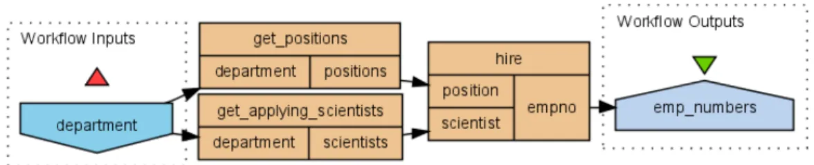
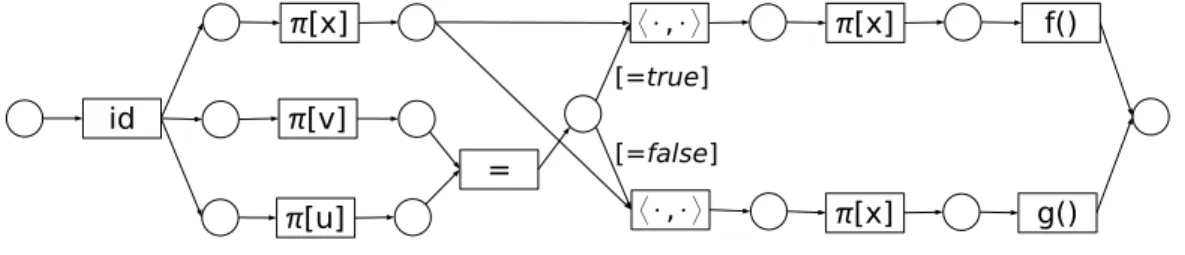
Figure 2.2: Recursive dot product motivation example
Fig. 2.2 where the initial value with an university department identifier, e.g., “informatics”, is used by two services, of which one produces a list of posi-tions available in this department and other a list of scientists applying for work there. The list of positions is sorted by their appeal and the scientists are sorted according to their achievements. A third service is used to hire a scientist for a position. To deal with the values of higher types it uses the
dot product strategy. This way the best positions are assigned to the best scientists and the hiring occurs while both positions and scientists are still available. Observe now that if this Scufl graph is executed with a list of de-partments identifiers, e.g., [“physics”,“bioinformatics”,“informatics”] and the implicit iteration over “get positions” and “get applying scientists” returned p = [[pp1, pp2],[pb1, pb2, pb3],[pi1, pi2]] and s = [[sp1, sp2, sp3],[sb1],[si1, si2]]
respectively, then the dot product of Taverna intermixes position and scien-tists from different departments, i.e., the worst physicist sp3 will be hired
on the best bioinformatics position pb1 and the best informatician si1 will
be hired on the worst bioinformatics position pb3. Even if it is the case
that informaticians and especially physicists do well as bioinformaticians, the informatics department becomes undermanned and does not get the best people. Clearly our recursive definition of dot product does not intermix the values, so scientists will only be hired by the departments they applied to and the departments will be able to hire all the scientists that applied to them as long as they have enough positions.
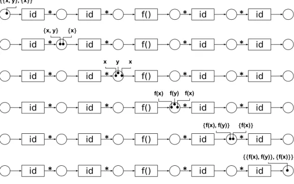
c£[[d;e];[f]] b£[[d;e];[f]] a£[[d;e];[f]] a[d
x
a b c d e f a[f a[e b[d b[e b[f c[d c[e c[fy
x
£
y
Figure 2.3: Cross product for higher list types
To understand the cross product of Taverna for higher list types it is convenient to think of the nested lists as ordered trees with the leaves labeled with tuple values. A tree interpretation of values x = [a, b, c] and y = [[d, e],[f]], where a, b, c, d, e and f are tuples, is given in Fig. 2.3. The cross product ofx and yis then obtained by replacing each of the leaf tuples tx in
xby a copy of theytree