EARN~GS AND EXPECTED RETURNS
Owen Lament
NBER Working Paper 5671
NATIONAL BUREAU OF ECONOMIC RESEARCH 1050 Massachusetts Avenue
Cambridge, MA 02138 July 1996
I thank Olivier Jean Blanchard, Kent Daniel, Eugene Fama, David Gross, Charles M. Jones, Steven Kaplan, Mark Mitchell, Jestis Sa6-Requejo, Robert Vishny, Paul Zarowin, Luigi Zingales, participants at the University of Chicago Finance Workshop, and especially John Cochrane for helpful comments, and Amy C. Ko for research assistance. I thank Roger Ibbotson for data. This work was supported by the FMC Faculty Research Fund at the Graduate School of Business, University of Chicago. This paper is part of NBER’s research program in Asset Pricing. Any opinions expressed are those of the author and not those of the National Bureau of Economic Research.
O 1996 by Owen Lament. All rights reserved. Short sections of text, not to exceed two paragraphs, may be quoted without explicit permission provided that full credit, including O notice, is given to the source.
July 1996
EARNINGS AND EXPECTED RETURNS
ABSTRACT
The aggregate dividend payout ratio forecasts aggregate excess returns on both stocks and corporate bonds in post-war US data. Both high corporate profits and high stock prices forecast low excess returns on equities. When the payout ratio is high, expected returns are high, The payout ratio’s correlation with business conditions gives it predictive power for returns; it contains information about future stock and bond returns that is not captured by other variables, The payout ratio is useful because it captures the temporary components of earnings. The dynamic relationship between dividends, earnings and stock prices shows that a positive innovation in earnings lowers expected returns in the near future, but raises them thereafter.
Owen Lament
Graduate School of Business University of Chicago 1101 East 58th Street Chicago, IL 60637 and NBER
As of May 1996, the dividend yield (D/p) on the Standard & Poor’s Composite Index about 2.2 %, which is remarkably low. This is remarkable because it implies negative
was
expected excess dividend yield.
stock returns, based on simple univariate forecasting regressions using the The price/earnings ratio (P/E) was about 19, which is not atypically high, and implies positive expected returns based on similar regressions. Which is right?
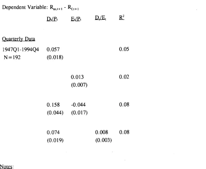
Shiner (1984) and Fama and French (1988) estimate regressions of returns on either lagged D/P or E/P, and find that both have explanatory power, but that D/P has more. Table 1 replicates the basic dividend yield and earnings yield regressions, using quarterly data on excess returns, dividends, and earnings from the Standtid & Poor’s Composite Index,
1947-1994. The first two rows show that the dividend yield does indeed produce better forecasts of future returns, compared to the earnings yield. The coefficient on the dividend yield is
significant and has more than twice the explanatory power of earnings yield. Fama and French (1988) explain these results: “Earnings are more variable than dividends.. .If this higher
variab i]ity is unrelated to the variation in expected returns, E/P is a noisier measure of expected returns than D/P. ”
Another way to compare the forecasting power of E/P and D/P is to put both in the same regression. 1 The third row in Table 1 shows that if one includes both E/P and D/P, the results appear unexpected: the dividend yield is still positive and significant, but now the earnings yield is negative and significant. What explains these results? The explanation must be that the higher variability of earnings mentioned by Fama and French (1988) is actually
‘ Campbell and Shiner (1988b) run annual excess return regressions with both E/P and D/P, 1871-1987, but only using a 30-year average of E (Table 2. B).
related to expected returns.
Thetworegressors are obviously related, since D/P = E/P *D/E. D/Eis the dividend payout ratio. Thethirdrow of Table 1 says that conditional onthe dividend yield, the
earnings yield is negatively correlated with future returns. One way of restating this fact is that conditional on the dividend yield, the dividend payout ratio is positively correlated with future returns. This restatement is shown in the last row of Table 1.
I proceed as follows. Section 1 documents that the payout ratio, conditional on the dividend yield, forecasts excess returns on equities. In Section 2, I consider why the payout ratio forecasts returns. In Section 3, I show that the payout ratio forecasts future dividends. I examine in Section 4 whether the payout ratio also forecasts excess returns on the bond market. Sect ion 5 looks at the payout ratio in relation to business conditions, and shows evidence cons istent with the idea that the payout ratio and the dividend yield are measures of two different determinants of expected returns: a “price” effect, which measures how high current stock prices are relative to some long-term average, and a “profit” effect, which
measures how high current profits are relative to some long-term average. Section 6 traces out the dynamic imp]ications of changes in earnings and dividends on prices. Section 7 examines the performance of dividend-free measures of the “price” and “profit” effects both in post-war quarterly data and in annual data 1871-1987. Section 8 provides evidence on the effects of repurchases on dividends in more recent years,
The main explanation for the payout ratio’s predictive ability is that the payout ratio is a good measure of current business conditions. Since expected returns vary over the business cycle, the payout ratio forecasts future returns.
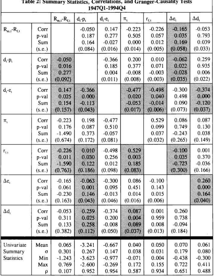
Table 2 shows (in the bottom row) basic summary statistics for the main series studied in this paper, and also presents (in the upper rows) bivariate Granger-causality tests and correlations across series. Here and for the rest of this paper, I use the natural log of the payout ratio and of the dividend yield (ln(D/E) = d-e, and ln(D/P) = d-p). Both the payout ratio and the dividend yield are based on quarterly data compiled by Standard and Poor’s, using the previous four quarter’s total earnings and dividends for the companies in the S&P Composite Index (additional information on these and other variables is given in the
Appendix). These two series are shown in Figure 1.
I focus on excess returns, the total (continuous y compounded) returns including reinvested dividends on the S&P
month treasury bills. Hereafter,
Composite Index minus the return on a portfolio of one-the word “return” means excess return over one-the riskless rate. 1’annualize returns so that the regression coefficients are comparable across different horizons .Z Table 2 also shows the three-month t-bill yield, the annualized CPI inflation rate, and growth rates of earnings and dividends as reported by S&P.
The main focus of this paper is on post-war data, since there are convincing reasons to believe dividend policy was very different in previous years. Section 7 discusses the issue of sample period in greater detail.
The shaded cells in Table 2 show when the series listed in the row Granger-cause the
a So that ~ = N * (ln(CSTIND,+~)-ln(CSTINDJ) where CSTIND is an index of total return as of the last day of month t. N= 12 for monthly data, 4 for quarterly data, and 1 for annual data.
interpreting the regressions presented later on. For now, it’s worth noting the payout ratio appears to be a very promising variable, in that it Granger-causes all the other variables (except Ae) and is Granger-caused by none.3
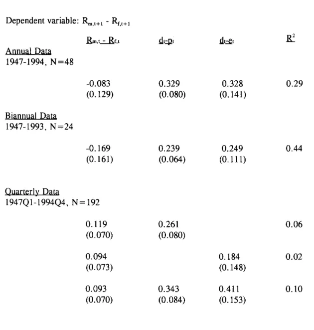
Table 3 shows quarterly, annual, and biannual regression of returns on dividend yield and dividend payout. I regress this period’s stock returns against last period’s payout ratio and dividend yield, and find that both the payout ratio and the dividend yield are helpful in
forecasting returns. The first two rows show the annual results and biannual results using non-overlapping observations; again, both the dividend yield and the payout ratio are significant explanatory of future returns, even with only 48 annual and 24 biannual observations. Inclusion of the payout ratio typically causes R2 to rise by about half again compared to a regression with only lagged returns and the dividend yield.4
The last three rows show quarterly results. I focus on quarterly results throughout this paper, since that is the frequency at dividends and earnings are reported. In regressions by themselves, both the dividend yield and the payout ratio are positively correlated with future returns, although the payout ratio is insignificant] y different from zero. The last row shows
5 Here and in Table 4, some caution should be used in interpreting regressions of Ae or Ad on its own lagged value and lagged e. In a regression of Ad on lagged Ad and lagged d-e, the inclusion of lagged d-e is equivalent to including twice lagged d-e and Ae lagged once. Interpretation is further affected by the fact that the quarterly observations on E and D are overlapping four-quarter moving averages, so naturally (as can been seen in Table 2) Ae and Ad are positively autocorrelated.
4 As a benchmark for the amount of explanatory power added by included the payout ratio, the biannual regressions with only lagged returns and the dividend yield has an R2 of 0.30 compared to 0.44 in Table 3.
the basic regression of this paper. When included in the same regression, the coefficients on both the dividend yield and the payout ratio rise; consequently, both are now positive and significant. Perhaps the fact (row 2) that the payout ratio is not a particularly impressive univariate predictor of returns (unlike the dividend yield) explains its hitherto obscure role in empirical asset pricing.
What does it mean that the payout ratio is not significant by itself, but only in the presence of the dividend yield? As shown in Table 2, d-e and d-p have a correlation of -0.37 during this period (the annual correlation is -0.41 ).5 Therefore, if both d-e and d-p “belong” on the right-hand side of the forecasting equation, it’s no surprise that omitting one variable causes the remaining variable to have a smaller estimated coefficient, due to omitted variable bias.’
In summary, both the payout ratio and the dividend yield appear to be positively and significantly correlated with future stock returns. The payout ratio is slightly less robust than the dividend yield, since it does poorly by itself. The Appendix studies the robustness of the
~The negative correlation of d-e and d-p implies that the temporary components (that is, the parts not explained by the cointegrating relationships) of p and e are negatively
correlated. For an individual firm, unexpected changes in earnings and stock prices are generally thought to be positively correlated. See, for example, Kormendi and Lipe (1987).
Table 2 shows that Ae and excess returns have a quarterly contemporaneous correlation of -O,17. The negative correlation holds both pre- and post-1970, although the negative correlation is much more intense in the latter period. Thus it is not solely a phenomena of the high inflation 1970’s. Real earnings growth and excess returns are also negatively correlated. I will return to this issue in section 6.
G Since R2 rises substantial y when d-e is included, it does not appear that collinearity between d-e and d-p is a serious problem. As further evidence on whether d-e and d-p measure the same thing, the R2 in a regression on one on the other is 0.13.
qu~terl y results, and finds that the results do not change much if one changes the sample period, changes the method of measuring the payout ratio, or excludes outliers.
2. Why Does The Payout Ratio Forecast Returns?
There appear to be four possible explanations of why the payout ratio forecasts returns. (1) The payout ratio forecasts returns not because it measures expected returns but because it measures future dividend growth, and thus “cleans up” the dividend yield as a measure of expected returns. (2) The payout ratio forecasts future returns because it is correlated with expected returns. (3) The payout ratio forecas~ future returns because it is correlated with fads, irrationality, or over-reaction by investors.7 (4) The payout ratio significantly forecast returns because it is one of the 5 % of irrelevant variables which have been found by academic data-dredging.
I attack these issues as follows. First 1 study the relationship between the payout ratio and future dividends and earnings. I consider whether the payout ratio is proxying for future dividend growth and not expected returns as in (1). I next test whether bond returns are forecasted by the payout ratio, since if (2) is true, one would expect the payout ratio to predict bond returns. I next consider whether the payout ratio is a business cycle variable that is likely correlated with discount rates, as in (2). I test whether the payout ratio contains information about future returns that is not present in other variables. In considering the business cycle and dynamic behavior of returns, I comment briefly on (3). I also examine whether one really needs dividends at all in order to capture the information present in both the payout ratio and
7 This might be the case if the payout ratio varies systematical y with the causes of fads (for example, over-optimism in good times, or over-reaction to current earnings).
the dividend yield.
As to point (4), I can say only that previous research and a long pre-scientific tradition have identified P/E and D/P as important variables predicting stock returns. If one believes that P/E and D/P measure expected returns, then it is important to understand their interaction.
3. The Payout Ratio, Dividends, and Earnings
A useful starting point is the simple Gordon (1962) model of stock prices:
P=~
r –g
where g is the growth rate of dividends and r is the discount rate, and both are fixed constants. Manipulation of the Gordon equation shows that D/P = r - g, so that D/P is a measure of both the discount rate and of future dividend growth. Campbell and Shiner (1988a) have a
dynamic, stochastic Gordon model:
where K is an unimportant constant. In the static Gordon model r =D/P + g, and in the
equal the required rate of return. The dividend yield is a good measure of one-period expected returns, but not a perfect measure, since it may be correlated with future returns and future dividend growth.
Using the Gordon model, it is easy to see that d-p is an noisy measure of E[rJ. It is plausible that d-e is correlated with the measurement error in d-p, since the measurement error in d-p depends on future dividend growth. If d-e were positively correlated with future
dividend growth but had zero correlation with expected returns, we would expect that d-e would spuriously appear with a positive and significant coefficient (since it is “cleaning up” the measurement error in d-p). 8
Is d-e positivel y correlated dividends follow a random walk.9
with future dividend growth? Some researchers find that If this
coefficient on d-e could not be caused by find that dividend growth is explained by
were the case, then the positive and significant its correlation with future dividend growth. Others lagged returns, lagged yields, and lagged earnings. 10
8 If this were the case, d-e would still be a useful variable for forecasting returns, but it would not reveal anything about stochastic discount rates.
g Froot and Obstfeld (1991), using S&P data 1900-1988, find that dividends follow a random walk; Adl is not explained by lagged Adt or by the lagged dividend yield. Cochrane (1994) uses annual CRSP data from 1927-1988 and finds dividends follow “nearl y“ a random walk and are not forecast by lagged dividends or yields.
‘0Marsh and Merton (1987) find that using annual CRSP data 1926-1980, Ad, is explained by lagged returns. Campbell and Shiner (1987, 1988b) find that Adt is explained by lagged dividend yields, lagged dividend growth, and a long average of the earnings price ratio using annual real S&P dividends 1871-1986. See also Kormendi and Zarowin (1994) for a cross-sectional anal ysis.
Table 2 shows that d-e Granger-causes Ad, using quarter] y data. However, the correlation of the dividend payout ratio and future dividend growth is negative: when the dividend payout ratio is low, dividends rise. 11 Thus the correlation of d-e and future dividend growth goes in the opposite direction needed for the simple “spurious” explanation of the ability of the payout ratio to forecast returns. 12
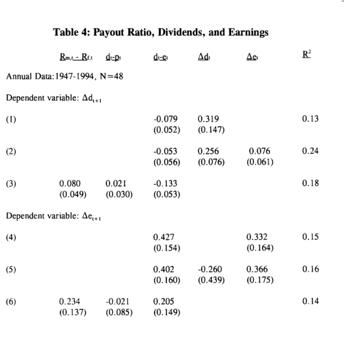
Table 4 shows that in annual data the payout ratio is negatively correlated with future dividends and positively correlated with future earnings, so that there is a simple error-correction model inherent in the relationship between these variables. Rows 1-3 certainly do not suggest that future dividends are completely unpredictable given current information. The correlation between d-e and future Ad appears somewhat weaker in Table 4 than in Table 2. Rows 4-5 suggest that the payout ratio is useful in forecasting future Ae, although the relationship again appears somewhat muddled in row 6 and in Table 2.
I conclude from the annual results in Table 4 and from the quarterly results in Table 2 that the payout ratio is possibly useful in forecasting future dividends and earnings.
As an alternate approach to the “cleaning up” issue, Kothari and Shanken (1992) regress current returns on realized future dividend growth and realized future returns, and on the lagged dividend yield. Kothari and Shanken find that the coefficient on D/P approximate] y doubles when one includes future dividend growth and future returns. Table 5 repeats this
‘‘ However, Blanchard (1993) finds the opposite result (p. 92).
‘z Of course, the negative relationship between d-e and future dividends in Table 4 is at the annual frequency. It could be that d-e is still positively correlated with future dividends at more long-term horizons.
exercise but includes the dividend payout ratio as well. Inclusion of either future dividends and returns, or future earnings and returns, does not appear to greatly affect the coefficients on the payout ratio and the dividend yield from Table 3. I conclude that the payout ratio does not appear to on]y reflect information about future dividends or earnings, but also information about future returns.
4. Interest Rate Spreads and Returns on Bonds and Stocks
If the payout ratio is correlated with time-varying discount rates, one would expect it to forecast returns on all risky assets, including assets not paying dividends.
Table 6 explores the ability of the dividend payout ratio to forecast returns on corporate bonds. Both the dividend yield and the payout ratio appear to be useful variables in
forecasting future bond returns. Both are positively correlated with future returns with coefficients ofs imilar magnitude; both are more than two standard errors from zero for the lower quality bonds.
Table 6 also shows the effect of two interest rate variables studied by Fama and French ( 1989). TERM, the term premium, is the difference between the AAA Corporate bond rate and the 1-month treasury bill rate. DEFAULT, the default premium, is the difference between the rate on a portfolio of “All” corporate bonds and the AAA Corporate bond rate. Table 6 also shows these interest rate variables in relation to excess returns on the S&P Composite Index and on a portfolio of small stocks.
Like Fama and French (1989), I find that TERM appears to be positive] y and
not vary much across assets. Like them, I also find that the dividend price ratio is positively and significant] y related to future returns on both stocks and bonds, with slope coefficients that increase with riskiness of the assets. I find that DEFAULT appears to contain no information (in addition to that already contained by d-e, d-p, and TERM) about future returns.’3
Like the dividend yield, the dividend payout ratio has a coefficient which generally increases with the riskiness of the asset. This suggests that the two variables play similar roles: both measure the required rate of return on risky assets. 14 The inclusion of DEFAULT and TERM generally reduces the coefficient on d-e somewhat. 15 For low-grade bonds and for the S&P Composite index, however, the payout ratio is still more than two standard errors from zero. I conclude that the payout ratio contains information about discount factors for risky assets that is not present in interest rate variables,
Fama and French (1989) interpret their interest rate spread results to mean that expected re[urns on stocks and bonds are lower when business conditions are strong. I next turn to examining whether the payout ratio predicts future returns for the same reason. The results of the next two sections suggest that the payout ratio is also a cyclical variable.
13Although the coefficient on DEFAULT increases with the riskiness of bonds, it has the wrong sign for stocks.
14The coefficient on the payout ratio is smaller for small stocks than for the S&P Composite index, although it is imprecise] y estimated. Removing TERM and DEFAULT from the small stocks equation results in a rise of the coefficient on d-e to about 0.300, although the standard error is stil I large so the coefficient is insignificant.
5. The Payout Ratio and Business Conditions
Both evidence and theory suggest that expected returns vary over the business cycle. ‘b While dividends are smooth, earnings are highly cyclical (the smoothness of dividends relative to earnings can be seen in Table 2, where dividend growth has half the variation of earnings growth). Lintner (1956) documents that managers engage in dividend smoothing, while Lucas (1977) lists as one of the seven main features of business cycles that “business profits show high conformity and much greater amplitude than other series. ” This means the payout ratio is a measure of business conditions. The payout ratio should be low when
earnings are strong and high when earnings are weak. This explains why the payout ratio has forecasting power for expected returns.
If this explanation is correct, then what matters for forecasting returns is not really the payout ratio per se, but rather the transitory component of earnings. Since the payout ratio happens to be an excellent measure of the business cycle and of the transitory component of earnings, it contains information about future returns.
The fact that both the dividend yield and the dividend payout ratio forecast returns
suggests that there are two components of expected returns. 17 When profits (measured by the payout ratio) and prices (measured by the dividend yield) are high, expected returns are low. call this latter effect a “price” effect rather than a “discount rate” effect to emphasize that it remains unclear whether the temporary components of stock prices can be rationalized by any
16For recent evidence, see Chen, Roll, and Ross Lucas (1978) and Campbell and Cochrane (1994).
17Fama and French (1989) and Cochrane (1991)
(1986), Chen (1991); for theory, see
make similar points.
remonable time-varying discount rate. In contrast, the “profit” effect appears to be readily understandable and fits in nicely with the desirable properties that a discount rate should have, since it is correlated with transitory components of income and presumably consumption.
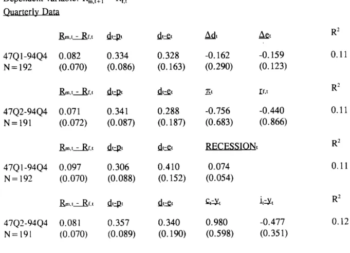
Table 7 investigates whether the payout ratio contains information that is not present in other variables that move over the business cycle.
First, Table 7 examines changes in earnings and dividends themselves. Adding
quarterly changes in dividends and earnings does not change much in the regression. Second, Table 7 examines short-term nominal interest rates and inflation. Figure 1 shows that the payout ratio was low in the 1970’s, when interest rates and inflation were high, and Table 2 shows that d-e is negatively correlated with interest rates and inflation. Bodie, Kane, and Marcus (1996) explain that the low P/E ratio’s in the 1970’s reflected “the market’s assessment that earnings in these periods are of ‘lower quality,’ artificial] y distorted by inflation, and warranting lower P/E ratios. ”
As shown in Table 7, inclusion of lagged inflation and lagged t-bill rates results in a decrease in the coefficient of the payout ratio. While neither the interest rate nor inflation variables are close to significant,
value of O.12. The payout ratio, p-value of 0.02. It is also useful
the coefficient on the payout ratio falls so that it has a p-inflation, and short-term rate are all jointly significant with a to recall from Table 2 that the payout ratio is helpful in forecasting future inflation and interest rates.
Third, Table 7 includes as a dummy variable equal to one if the quarter contains a month between business cycle peak and trough, as defined by the National Bureau of Economic Research, This variable, RECESSION, has little effect on the results. Fourth,
Table ‘7includes two ratios which move over the business cycle: the log of the consumption GDP ratio, and the log of the investment to GDP ratio. la Again, including these variables
to
lowered the coefficient and raised the standard error on the payout ratio, so that d-e now has a p-value of 0.08. Again, the payout ratio, the investment ratio, and the consumption ratio are all jointly significant with a p-value of 0.02.
I conclude from Table 7 that there is some evidence that the payout ratio reflects the same information already present in other business cycle variables, namely inflation, interest rates, consumption, and investment. Inclusion of these variables primarily raise the standard error of the estimated effect of the payout ratio, as the coefficient stays around .3. While the payout ratio is not as robust as the dividend yield, it still appears to be useful information.
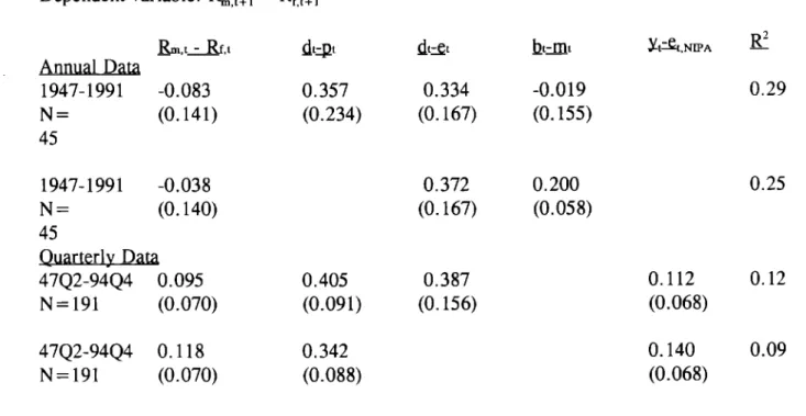
Next, here and in section 7, I test the conjecture that profit and price (as opposed to dividends) matter by dispensing with the dividend yield or the payout ratio and attempting to find other variables that capture the fact that dividends are simply a slowly-moving average adjusting to changes in future earnings. Table 8 shows the results.
First, using annual data, I include the ratio of the book value of the S&P Index to the market value. 19 As the first regression shows, the market-to-book ratio appears to contain no information that it is not already present in the dividend yield .20 Dropping the dividend yield,
‘8The consumption to GDP ratio is the same variable used in Cochrane (1994); the investment to GDP ratio is similar but not identical to the variable in Cochrane (1991).
19This market to book is based on the S&P Industrial Index, which has a longer time-series for book value than the Composite Index.
20This is not surprising for postwar data, given the evidence in Kothari and Shanken—
I find that the market-to-book ratio does a tolerable job of capturing the effect of high stock prices on future returns.
Next, using quarterly data, I replace the payout ratio with a GDP-based measure of whether current profits are “high” relative to some more SIOWIy moving benchmark. I use the ratio of profits after tax reported by the corporate sector to the gross domestic product of the corporate sector. Alongside the payout ratio, this variable is insignificantly different from zero. Dropping the payout ratio, this variable does a fair job replicating the effect of the payout ratio.
The lesson from Table 8 is that there appear to be two separate determinants of time-varying expected returns. The first variable measures how high current prices are relative to slowly-moving measures of value like dividends and book value. This is the component of stock market predictability that has received the most attention (e. g., from Shiner (1984), and Fama and
reflect the relative to
French (1988)). The mean-reverting properties of stock prices presumably also presence of this effect. The second variable measures how high current profits are some slowly moving average like dividends or corporate product, In that profits are a cyclical variable, the “profit effect” has been documented by Fama
(1991), and others.
If this pattern were due to over-reaction of prices to earnings,
and French (1989), Chen
we ‘d expect to see
positive contemporaneous correlation of Ae and returns, which we do not observe in the data. 2’
2’ What we obsene is a negative correlation that is sometimes statistically significant (if measured as a simple univariate correlation or in Table 5), but insignificantly different from zero in the VAR estimated in the next section.
So it is not obvious how a simple overreaction story the price effect is still an open question. The payout
fits in with the profit effect. Of course, ratio (along with interest rate variables) purges the dividend yield of its cyclical variation. So the dividend yield represents the discount rate changes that are not explained by changes in risk aversion induced by the business cycle. Thus, there must be changes to the covariance of marginal utility and returns which remain mysterious in origin.
6. Dynamics of Dividends, Earnings, and Prices
One way to summarize the data and its implications is by estimating a vector
autoregression (VAR). Impulse response functions from a VAR show the dynamic effect of an innovation in one variable on the other variables in the system.
This section relies heavily on Cochrane (1994). He studies a bivariate system consisting of dividends, prices, and a cointegrating vector (d-p). The inclusion of an error correction term, d-p, forces dividends and prices to move together in the long-term. ‘z
In the present paper, there are three variables of interest and two long-term
relationships. I therefore study a system consisting of three variables, dividends, earnings, and prices, and two cointegrated vectors (d-p and d-e). This system with two restrictions is
equivalent to an unrestricted VAR in three variables: returns (~-R~), dividend yield (d-p), and the payout ratio (d-e). 23
I estimate this unrestricted VAR, using quarterly data from 1947Q1 to 1994Q4, and
22And is predicated on the “ Cochrane (1994) p. 262.
assumption that the dividend yield is a stationary variable. These procedures are equivalent up to a lag length restriction, and under the assumption that d-p and d-e are stationary.
using four quarters of lags. Figure 2 shows the estimated effect of the three types of
innovations innovations to returns, to the dividend yield, and to the dividend payout ratio -on cumulated excess returns. Figure 2 shows the standard impulse response function of excess returns to these three variables, but summing the estimated response over time. Following Cochrane (1994), these responses can be thought of as the response of (de-trended) stock prices to the different shocks.
In Figure 2, I have ordered the data (d-e, d-p, ~-R~) so that changes in the payout ratio can have a contemporaneous effect on prices, and I have arranged the figure so that it shows shocks corresponding to an increase in prices, dividends, and emnings. w The figure shows that the effects of dividend and price shocks on stock prices are quite similar to the ones Cochrane estimated (using annual data 1927-1988).
prices. But this increase in prices is self-correcting;
A price shock obviously the price level gradually
initially increases returns to the level iLwas forecasted to reach before the price shock occurred (it takes about five years for the innovation to die out). In this sense, price shocks are transitory. A dividend shock also increases prices. But this increase in prices appears to be permanent; a rise in stock prices that is accompanied by a rise in dividends never reverses itself.25
“ An “earnings shock” is a shock to d-e; a shock to earnings that is not accompanied by a change in dividends.
‘5 Some VAR systems are highly sensitive to the ordering (the orthogonalization assumption) of the variables in the system. Fortunate] y, this one is not. Therefore, consider the following ordering of the variables: (d-p, ~-R~, d-e). Placing d-p first is equivalent to placing the contemporaneous dividend yield in the equation for excess returns.
Consider a change in the price of stocks. If this change is not accompanied by a change in dividends, then this price change results in an innovation in the dividend yield. Following Cochrane, call this type of shock a “price shock. ” A price shock is a change in the
In terms of their impulse response function, earnings shocks appear to occupy a middle ground between dividend shocks and price shocks. Like price shocks, earnings shocks are not permanent, and complete] y die out after about five years. Unlike price shocks, earnings shocks initially grow (over the course of six quarters) instead of gradual] y decaying.
Stock prices fall when an earnings shock arrives (this contemporaneous decline in stock prices is less than two standard errors from zero). Stock prices continue to fall (relative to trend) for the next year or two. The decline in stock prices in the quarters immediately following the innovation in earnings is more than two standard errors away from zero, using standard Monte Carlo methods to calculate standard error bands. These results from the VAR are consistent with the evidence in Tables 2 and 3.
The time pattern of the response of returns to earnings shocks - initially falling in response to an increase in earnings, then rising - corresponds to business cycle variation in expected returns. An innovation in earnings means good times. The discount rate is thus below average. Since there is some short-term persistence of business conditions, prosperity continues on for six to eight quarters, but then starts to fade. As the business cycle turns sour, times are no longer good. Therefore, expected returns rise, since the discount rate is now above average. Eventually stock prices return to the level at which they were originally forecast before the innovation in earnings. After four or five years, the net effect of the
dividend price ratio. Now consider the second variable in the system, excess returns. Since putting d-p first in the ordering is equivalent to putting the current yield in the returns
equation, an innovation in returns is a change in price which is not accompanied by a change in the yield. In other words, it’s a change in price that is accompanied by a change in dividends, So call this type of a shock a “dividend” shock. A dividend shock is a change in returns that is not caused by changes in the dividend yield.
innovation in earnings has died out. Since discount rates vary with the business cycle, they vary at business cycle frequencies, which is exactly what Figure 2 shows.
So much for the reaction of future prices to an innovation in current earnings. What about the contemporaneously negative correlation of earnings and returns? Although this correlation is not statistically robust, it is interesting to see if it can be explained using existing models. It can be.
According to the Campbell-Shiller (1988a) dynamic Gordon equation, an unexpected positive innovation in earnings will have two effects. First, the Lintner model (and Tables 2 and 4) says a rise in earnings means that dividends are likely to rise in the future, so stock prices should rise. The second effect of an innovation in earnings is to change the expected path of future returns.
fall. So the net effect
If expected discount rates rise enough in the future, stock prices will on stock prices is ambiguous.
Let AE be the revision in expectations induced by the innovation in earnings. Suppose that the innovation in earnings causes an downward revision in expected discount rates from now unt i1date N, and an upward revision in expected discount rates thereafter. If:
N
then current stock prices will fall in response to an unexpected increase in earnings.
7. Dividend-free
Measures of Prices and Profits
The main focus of this paper is the predictability of quarterly asset returns using the dividend payout ratio in postwar US data. We know how dividends are set empirically (at least for the postwar period). As Lintner (1956) documented in a series of classic interviews, most managers have a target level of dividends equal to a fraction of some “permanent” level of earnings. When the “permanent” level of earnings changes, managers S1OWIy adjust their dividends toward the new target level. But we do not know why dividends are set this way, although we have some good ideas. As Modigliani and Miller (Modigliani and Miller (1958), Miller and Modigliani (1961)) show, there are good reasons to believe dividend policy could be set in any arbitrary fashion without serious consequence.
Since (a) dividends are a smoothed, (partially) forward-looking measure of the future earnings of the firm, and (b) the market value of the firm is the discounted value of the future earnings of the firm, it is no surprise that (as shown in the previous section) a change in
aggregate dividends is typical Iy accompanied by a permanent change in the market value of the aggregate stock market. This paper documents that the discount rate used to calculate the discounted value of future earnings in (b) is actually affected by the current level of earnings.
However, (a) is not a law of nature, theorem, axiom, or definition. It is merely an empirical regularity with ill-understood origins. Therefore it might change in the future and might not have been true in the past. Black (1976) asks “Why do corporations pay dividends? Why do investors pay attention to dividends?” Widely-agreed upon answers to these questions still do not exist.
In the next section, I discuss evidence that in fact dividend policy has not changed much in the past decade (although corporate distribution of cash to shareholders has). However, it would still be useful to have measures of expected returns that do not rely too much on dividends, since it is conceivable that dividends are a historical y transitory
phenomenon.zs There are reasons to believe that changes in tax policy and the institutions of corporate governance can cause dividend policy to change. Managers might stop smoothing dividends, or might smooth them so much that they contain little information. In this case, the payout ratio would become less useful.
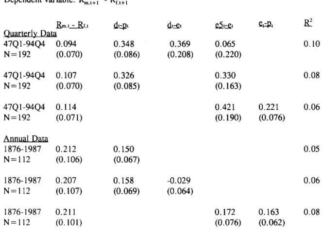
The finding of this paper is that high prices and high profits are associated with low future returns. If these results are based on fundamental principles of human nature, then they should hold in all periods, not just in postwar data, In postwar data, both the price effect and the profit effect can be well measured using dividends in the numerator. There are reasons to think that dividends will be unreliable in prewar data.
In Table 9, I therefore construct measures of prices and profits that are dividend-free. To replace the numerator in the payout ratio, I construct a backward-moving average of quarterly earnings, using the average of (arbitrarilyy) the past five years of earnings. To replace the dividend yield term, I use the earnings yield. The third line of the table shows the
‘GFor example, the Microsoft Corporation has never in its history paid a dividend, and needn’ t pay one for the next 100 years. If all publicly traded companies follow Microsoft’s example, the dividend price ratio and the dividend payout ratio will have zero mean and zero variance (at least in small samples), and the log of these variables would be negative infinity. This would render less relevant several decades of research, including the theory and evidence of Gordon (1962), Shiner (1984), Fama and French (1988), Campbell and Shiner (1988a,
In terms of explanatory power, this regression does worse than regressions which include dividends, since the past five years of earnings is evidently an inferior measure of the permanent component of earnings. Nonetheless, the regressions confirm the basic point: high P and high E are both negatively correlated with future returns.
I focus on post-war data in this paper for two reasons. First, previous research has found a substantial change in dividend-smoothing by firms over time.27 Second, the
Undistributed Profits Tax of 1936-1937, which taxed retained earnings and thus raised firms’ incentive to pay dividends, undoubted] y had an effect on the dividend payout rate. 2s The dividend price ratio rose from 3.4 % at the end of 1935 to over 7% at the end of 1937. The tax-induced distortions surely affect empirical attempts to explain dividend price ratios and returns in this period.
A full investigation of the prewar evidence is beyond the scope of this paper. Table 9 contains exploratory results, and uses annual data 1871-1987 from Shiner (1989) to test both whether the price and profit effects are present in the entire sample, and whether these effects
27Using annual CRSP data, Fama and French (1988) find that the variability of A4
falls more between 1926-56 and 1957-86 than the variability of returns and AeL. They also find that the speed of adjustment of E to D falls in the latter period. boking at annual S&P data, Barsky and De bng (1989) reject the hypothesis that the volatility of dividend growth was constant between 1880-1939 and 1940-1981.
26See Calomiris and Hubbard (1995) for details on this episode, which is also mentioned in Lintner (1956).
are well captured by the dividend yield and the dividend payout ratio. ‘g
effects are long-term phenomena,
does Table 9 shows that the dividend payout ratio performs abysmally during the 1871-1987 sample period, having an estimated effect of about zero. The dividend-free specification much better, and explains more of the variation in returns than the specification using dividends.
Table 9 suggests that the price and profit effects are fairly stable over time. Throwing away dividend information is not a terrible idea for the past century of dam.
the price and profit
8. Repurchases
I conclude that
Bagwell and Shoven (1989) document that repurchases greatly increased in the mid-1980’s.3(’ Repurchases might affect the results in two ways. First, if stock repurchases replace dividends, then the past history of dividend yields and dividend payout ratios will be a
mislead ing guide to future stock returns. Second, if repurchases were an important phenomena in the sample period, they might be affecting the dividend yield and dividend payout ratio results .31
‘9These regressions are not exactly analogous to the previous ones because the
available data does not permit calculation of total return including reinvested dividends within the year.
30Aside from repurchases, another recent phenomenon may also be affecting dividend payout ratios. Hines (1996) documents that the payout ratio increases with the foreign income of US firms.
3’ For example, if managers repurchase stock instead of paying dividends when they know that the stock market is undervalued, then both the dividend yield and the dividend payout ratio would be negatively correlated with future stock returns.
Figure 1 does not suggest that repurchases lowered the dividend payout ratio in the mid-1980’s. If anything, the payout ratio rises around the mid-1980’s. Allen and Michaely (1995), citing evidence from Dunsby (1995), conclude that repurchases do not appear to significantly substitute for dividends; instead, repurchases represent an increase in the total cash payout to stockholders.
Using aggregate data on repurchases, I tested whether the repurchases to earnings ratio, rp-e, was affecting the results on d-e or d-p.32 First, I note that the correlation between rp-e and d-e is positive (O.24 from 1973-1994), so it does not appear that dividends are crowded out by repurchases. Second, repeating the basic annual regression from Table 3 using data
1973-1994, the inclusion of rp-e has little effect on the coefficients on d-e or d-p, and rp-e is itself small and statistically insignificant.33 I conclude that repurchases are not driving the results, have not in the past been useful in forecasting aggregate returns, and so do not need to be taken into account when constructing forecasts of future returns .34
3ZI measured rp-e using the Dunsby (1995) Compustat-based data reported in Allen and Michael y (1995) for 1973-1991 and additional 1992-1994 data based on aggregate estimates from Poterba and Samwick (1995). These measures of rp-e are based on a different sample of companies than the S&P 500.
33Adding rp-e to the annual regression 1971-1994 causes the coefficient on d-e to fall from 0.42 to 0.36. The standard error on the coefficient is 0.26. The coefficient on rp-e is 0.03 with a standard error of 0.04.
34In addition to the data on repurchases, the evidence from Tables 8 and 9 suggests that one can more or less measure the price and profit components of expected returns without resort to dividends, so it cannot be changes in the distribution of earnings that are
9. Summary and Conclusion
The payout ratio predicts expected returns on both stocks and bonds. It is probably the payout ratio’s correlation with time-varying discount factors that gives it predictive power for returns. The dividend yield and the dividend payout ratio measure two different time-varying components of expected returns. The first component is that when prices are high, expected returns are low. Second is that when profits ue high, expected returns are low.
The evidence presented here does not pose a challenge to existing theory. The resulk do have practical implications, however. In particular, I have presented evidence that the following statements are false. (1) As of 1996, dividend yields are not a good indicator of future stock returns because repurchases have replaced dividends. (2) The best way to use earnings information to forecast stock returns is to discard current earnings and average past earnings over long periods of time. (3) If one has D/P, one does not need E/P to forecast stock returns, since E/P is simply a more noisy measure of same thing D/P measures. (4) The very low forecasts of expected returns based on D/P as of early 1996 should be moderated by the fact that E/P is not very low. (5) Aggregate stock prices rise in response to an increase in aggregate earnings.
In general, there is no good reason to expect the time-series and cross-section evidence to be precisely analogous, since the profit effect is probably caused by aggregate attitudes toward risk. Nonetheless, it is interesting to note that some researchers examining cross-sectional expected returns have found that earnings are sometimes negatively correlated with
future returns at the level of an individual firm .35
Earnings are a useful variable.3b We almost certain] y have better measures of corporate accounting earnings than we have of aggregate consumption, especially for the 19th century. So at a minimum, earnings can serve as a convenient measure of business conditions and therefore of expected returns.
I conclude from the evidence that dividends are neither necessary nor (in pre-war data) sufficient to document the price and profit effects. In postwar data however, aggregate
dividends appear to be the most useful and forward-looking measure of the long-run components in both stock prices and corporate earnings.
35Lakonishok, Shleifer, and Vishny (1994) find that stocks with both a high price and high recent rate of growth - “glamour stocks” - have low future returns. In their terms, periods when the aggregate stock market has both a high price and high earnings might be called “glamour periods. ” As previously discussed, the negative correlation of prices and earnings makes the “glamour” interpretation difficult for time-series. Jaffe, Keim, and Westerfield (1989) find that, “surprisingly,” US firms with negative earnings have higher expected returns. After looking at the time series evidence presented here, these results are still surprising (since presumably much of the variation in earnings across firms is
idiosyncratic) but at least more familiar. Looking at the cross-section of Japanese stock returns, Chan, Hamao and Lakonishok (1991) report results eerily similar to the ones presented in Table 1:
“If earnings yield is considered in isolation . . .it indeed has apositive and
significant impact on returns. If the book to market ratio is added to the model, however, the coefficient becomes insignificant y different from zero. In the context of the full model, earnings yield even has a negative impact on stock returns, and is in some cases reliably negative. ”
36I agree with Campbell and Shiner (1988b) that “many studies of financial time series have avoided the use of earnings data and have thus omitted relevant information about
Appendix: Data, and Robustness of the Quarter]y Results
DataAll data on stock, bond, and bill returns come from Ibbotson Associates. The basic earnings and dividends data are from the Securi~ Price ltiex Record published by Standard & Poor’s Statistical Service. Earnings per share is 4-quarter total, Adjusted to Index, Composite. Dividends per share is 12-months moving total, Adjusted to Index, Composite.
Examining regressions of various variables on seasonally dummies, there is no evidence that the d, e, Ae, Ad, d-p, or d-e series have a seasonal component.
Other measures of the payout ratio
In Table A, I replicate the quarterly results of Table 3 using four different, alternative measures of lagged dividend payout. All of these measures have slightly different time aggregation properties.
First, I use the quarterly corporate dividend and after-tax profit figures reported in the National Income and Product Accounts to construct dtF~lPA-e,,mA.These accounts are designed to reflect seasonally-adjusted economic transactions for the entire corporate sector within the quarter, and so in principle are different from the moving average of the last four quarters for just the S&P companies. Second, I use the “actual quarterly” earnings reported by S&P,
E~,~~~,instead of the four-quarter total. 37 I did not attempt to seasonally adjust this variable. The third and fourth variables attempt to correct for timing issues in the release of the S&P
quarterly figures. quarter until well
Companies (and therefore S&P) do not announce their earnings for a given into the next quarter. Thus the exact value of E, is not in the information set of agenw at time t. 3s I therefore tried using d-e lagged an additional quarter. Last, I used “real-time” D/P and E/P information reported by S&P concurrent] y, d~,RT-e~,RTand di,RT-pL,RT. extracted this information from Citibase. 39
I
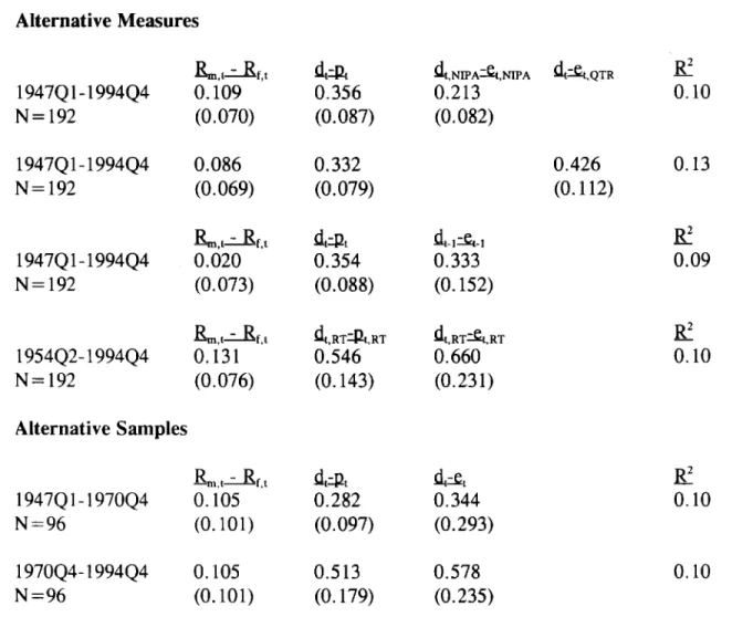
As can be seen in Table A, these different measures of the lagged payout ratio had little effect on the qualitative conclusions about yields, payouts, and returns.@ Notice that using E,,~~R,the “noisy“ measure of current earnings, actually causes both the coefficient on the payout ratio and the explanatory power of the regression to rise, This finding echoes results elsewhere in this paper: changes to the payout ratio are temporary changes in earnings, which explains why they forecast returns, Since Et,~TRis an even better measure than Et of transitory shocks to earnings, it is not surprising it does a good job of explaining variations in expected returns.
Subsamples
Cutting the quarterly sample in half, as shown in Table A, does not appear to result in
38This is a feature of all studies that use earnings data, not just this one. For example, the extremely useful data series contained in Shiner (1989) are also contaminated in this fashion.
39Unfortunate y, Citibase reports month]y averages of weekly indices, so the
constructed payout ratio is a noisy measure of the actual end-of-quarter payout ratio known at time t. The weekly P/E series is also only available from S&P starting in 1954.
@The higher coefficients on d,,RT-eL,~Tand d,,RT-pL,RTare due entirely to the different sample period; using the same sample period and regularly defined d-e and d-p yields very similar results.
dramatic differences in the relationship between the payout ratio and returns. Although the estimated coefficient is statistically insignificant in the first half of the sample, the size of the coefficient is about the same as in the full sample. I conclude that the relationship between payout and return is probably not an artifact of the inflation of the 1970’s, the 1987 crash, or the repurchases of the 1980’s and 1990’s .41
Outliers
Folk wisdom appears to associate low dividend yields not onl y with low returns, but also with negatively skewed returns. For example, in considering the early 1996 dividend yield (a record low), it is natural to draw apocalyptic parallels to the last time the dividend yield was very low: the period immediately preceding the 1987 crash. Is the statistical relationship between dividend yields, payouts, and future returns caused primarily by a few ou(1iers Iike October 1987? The answer is no. Removing return observations that are two standard deviations away from the mean results in little change in benchmark quarterly results of Table 3 .J: Both the univariate regressions and bivariate regressions of returns on e and d-p look about the same in terms of coefficients and (surd-prisingly) R’. The one difference is that d-e is now significantly different from zero by itself, with a coefficient of 0.244 and a standard error of O.122. I conclude therefore that skewness in returns is not responsible for gross!y distorting the linear regressions.
41I also discuss these issues elsewhere in the paper.
42There were seven such quarters in the sample period, five of which were price declines.
Miscellaneous Robustness
Table 3 shows simple OLS regressions and standard errors. Using Newey-West errors with one lag does not change the conclusions from Table 3 (the standard error on d-e rises somewhat to O.172). Using real returns or nominal returns instead of excess returns also results in little change.
References
Allen, Franklin, and Roni Michael y, “Dividend Policy, ” in Finance, edited by R.A, Jarrow, V. Maksimovic, and W.T. Ziemba, Amsterdam: Elsevier, 1995.
Bagwell, Laurie Simon and John B. Shoven, “Cash Distribution to Shareholders, ” Journal of Econonzic Perspectives, Summer 1989, Vol 3 No 3 pp. 129-140.
Barsky, Robert B., and J. Bradford De Long, “Why Does the Stock Market Fluctuate, ” Quarterly Journal of Economics, May 1989, Vol CVIII, Issue 2, pp. 291-312.
Black, Fischer, “The Dividend Puzzle, ” Journal of Po&olio Management, vol. 2, Winter 1976, pp. 5-8.
Blanchard, Olivier J., “Movements in the Equity Premium, ” Brookings Papers on Economic Activi~, 1993:2, 75-138.
Bodie, Zvi, Alex Kane, and Alan J. Marcus, Investments, Chicago: Irwin, 1996.
Calomiris, Charles W., and R. Glenn Hubbard, “Internal Finance and Investment: Evidence from the Undistributed Profits Tax of 1936-7, ” Journal of Business, October 1995, Vol 68 No 4 pp.443-482.
Campbell, John Y., “A Variance Decomposition for Stock Returns, ” Economic Journal, March 1991, 101:157-179.
Campbell. John Y. and John H. Cochrane, “By Force of Habit: A Consumption-based Explanation of Aggregate Stock Market Behavior, ” CRSP WP 412, December 1994.
Campbell, John Y. and Robert J. Shiner, “Cointegration and Tests of Present Value Models, ” Journal of Political Economy, 1987, 95, pp. 1062-1088,
Campbell, John Y. and Robert J. Shiner, “The Dividend-Price Ratio and Expectations of Future Dividends and Discount Factors, ” Review of Financial Studies, 1988a, Vol 1, No 3 pp.
195-228.
Campbell, John Y. and Robert J, Shiner, “Stock Prices, Earnings, and Expected Dividends, ” Journal of Finance, 1988b, 43, pp. 661-676.
Chan, Louis K. C., Yasushi Hamao, and Josef Lakonishok, “Fundamentals and Stock Returns in Japan, ” Journal of Finance, 1991, Vol XLVI, No. 5, 1739-1764.
Finance, June 1991, Vol. XLVI, No. 2, pp. 529-554,
Chen, Nai-Fu, Richard Roll, and Stephen A. Ross, “Economic Forces and the Stock Market, ” Journal of Business, 1986, Vol. 59, No.3, pp. 383-403.
Cochrane, John H., “Production-Based Asset Pricing and the Link Between Stock Returns and Economic Fluctuations, ” Journal of Finance, 1991, VOI. XLVI, N0. l,pp. 209-237.
Cochrane, JohnH., “Explainingt heVariance of Price-Dividend Ratios,’’ Review ofFinancial Studies, 1992, Vol. 5, No.2, pp. 243-280.
Cochrane, John H., “Permanent and Transitory Components of GNP and Stock Prices, ” Quarterly Journal of Economics, February 1994, Vol. CIX Issue 1, pp. 241-266.
Dunsby, Adam, “Share Repurchases, Dividends, and Corporate Distribution Policy, ” University of Pennsylvania Ph.D. dissertation, 1995.
Fama, Eugene F. and Kenneth R. French, “Dividend Yields and Expected Stock Returns, ” Journal of Financial Economics, 1988, 22, pp. 3-25.
Fama, Eugene F. and Kenneth R. French, “Business Conditions and Expected Returns on Stocks and Bonds, ” Journal of Financial Economics, 1989, 25, pp. 23-49.
Froot, Kenneth A. and Maurice Obstfeld, “Intrinsic Bubbles: The Case of Stock Prices, ” American Economic Review, December 1991, Vol 81 No 5, pp. 1189-1214.
Gordon, M. J., me Investment, Financing, and Valuation of the Corporation, Irwin, Homewood, Ill. 1962.
Hines, James R. Jr., “Dividends and Profits: Some Unsubtle Foreign Influences, ” Journal of Finance, 1996, 51, 661-689.
Jaffe, Jeffrey, Donald Keim and Randolph Westerfield, “Earnings yields, market values and stock returns, ” Journal of Finance, 1989, 44, 135-148.
Kormendi, Roger, and Robert Lipe, “Earnings Innovations, Earnings Persistence, and Stock Returns, ” Journal of Business, 1987, Vol. 60 No. 3, pp. 323-345.
Kormendi, Roger, and Paul Zarowin, “The Permanent Income Hypothesis of Corporate Dividend Policy: Empirical Tests, ” June 1994 NYU working paper.
Kothari, S. P. and Jay Shanken, “Stock return variation and expected dividends: A time-series and cross-sectional anal ysis, ” Journal of Financial Economics, 1992, 31, pp. 117-210
Kothari, S.P. and Jay Shanken, “Book-to-market, Dividend Yield, and Expected Market Returns: A Time Series Analysis, ” August 1995 working paper.
Lakonishok, Joseph, Andrei Shleifer, and Robert W. Vishny, “Contrarian Investment, Extrapolation, and Risk” Journal of Finance, 1994, Vol XLIX, No. 5, 1541-1578. Lintner, John, “Distribution of Incomes of Corporations Among Dividends, Retained Earnings, and Taxes, ” American Economic Review, May 1956, 46:97-113.
Lucas, Robert E., Jr, “Understanding Business Cycles, “ in Stabilization of the Domestic and International Economy, Carnergie-Rochester Series on Public Policy vol. 5, eds. Karl Brunner and AlIan H. Meltzer, Amsterdam: North-Holland Publishing Compnay, 1977, pp. 7029. Lucas, Robert E., Jr, “Asset Prices in an Exchange Economy, ” Economettica, 1978, 46, pp.
1429-1445.
Marsh, Terry A. and Robert C. Merton, “Dividend Behavior for the Aggregate Stock Market, ” Journal of Business, 1987, Vol. 60 no. 1, pp. 1-40.
Miller, Merton H. and Franco Modigliani, “Dividend Policy, Growth, and the Valuation of Shares”, Journal of Business, October 1961, 34, pp. 411-33.
Modigliani, Franco and Merton H. Miller, “The Cost of Capital, Corporation Finance and the Theory of Investment”, American Economic Review, June 1958, p. 261-97.
Poterba, James M. and Andrew A. Samwick, “Stock Ownership Patterns, Stock Market Fluctuations, and Consumption, ” Brookings Papers on Economic ActiviQ, 1995:2, 295-372. Shiner, Robert J., “Stock Prices and Social Dynamics, ” Brookings Papers on Economic ActiviQ, 1984:2, 457-498.
Table 1: Excess Return vs. Dividend Yield, Earnings Yield, and Payout
Q
uarterlv Dau 1947Q1-1994Q4 0.057 0.05 N=192 (0.018) 0.013 (0.007) 0.02 0.158 -0.044 0.08 (0.044) (0.017) 0.074 0.008 0.08 (0.019) (0.003) Notes: %,[+1 - Rf,l+l = 4 * (ln(CSTIND~+l)-ln(CSTINDJ)-4*(ln( USTINDL+1)-ln(USTIND)) inquarterly data, where CSTIND is an index of total return (including reinvested dividends) on the S&P Composite Index and USTIND is an index of total return on one-month T-bills, as of the last day of quarter t. D, E, and P are the quarterly dividends, earnings, and end-of-period stock price levels reported by Standard and Poor’s Statistical Service. Earnings and dividends are 4-quarter totals, paid out in the four quarters including quarter t. All regression in this and other tables include a constant term, not shown.
Table 2: Summary Statistics, Correlations, and Granger-Causality Tests 1947Q1-1994Q4 Tt, Corr -0.223 0.198 p-val 0.176 0.087 Sum -1.490 0.373 (se.) (0.674) (O.172) Univariate Mean 0.065 -3.241 Summary o 0.301 0.267 Statistics Min -1.243 -3.623 Max 0.769 -2.600 P 0.107 0.952 0.147 0.277 -0.027 (0.016) -0.366 0.185 0.004 (0.011) -0.477 0.510 -0.057 (0.081) -0.498 0.256 0.012 (0,098) -0.300 0.095 -0.013 (0.046) -0.374 0.200 -0.008 (0.050) -0.667 0.147 -0.977 -0.269 0.954 nt -0.223 0.505 (o”o~ 0.529 0.086 0.087 0.099 0.749 0.130 0.037 -0.243 0.038 (0.032) (0.265) (0. 149) ,,,,..,.,... :.:.:.:::-,,.:::.:.:::-::-::.{;:’.,::fi::,. .,.,,,...,,,,,.,..,.... 0.001 0.260 0.959 0.738 0.008 -0.094 (0.013) (O.184) 0.050 0.070 0.061 0.031 0.179 0.080 0.004 -0.438 -0.300 0.155 0.722 0.411 0.934 0.651 0.488
Notes to Table 2: “Corr” is the correlation coefficient between the two variables. “P-val” is the p-value from a Granger causality test for whether the variable in the row G-causes the variable in the column. This is a test of whether four lagged quarters of the row variables can be excluded from a linear regression where the dependent variable is the column variable and the independent variables are four lags of the column and row variables. “Sum” is the sum of the four quarter] y coefficients on the lagged row variable in this regression. “s. e.” is the standard error of the estimate of this sum. u is the standard deviation of the column variable and p is its first-order autocorrelation coefficient.
r~,fis the three-month t-bill rate at end of quarter t, whereas R~~is the ex-post return on a portfolio of one-month t-bills, rolled over in the course of three months of quarter t. n, is the annualized quarterly inflation rate, using the difference in log of the CPI index provided by Ibbotson Associates. Aet and Ad, are the annualized change in the log of the four quarter total of earnings per share and dividends per share, between quarter t-1 and quarter t, as reported by Standard and Poor’s.
The shaded cells of the table signify that the p-value (from a Granger causality tests for whether the variable in the row G-causes the variable in the column) is below 0.05.
Table 3: Excess Returns and the Payout Ratio
Dependent variable: K,,+l - Rf,t+I&,taf,t dtqt dtat Annual Dm 1947-1994, N=48 -0.083 (0.129) Biannual DaQ 1947-1993, N=24 -0.169 (O.161) Ouarterly Da~ 1947Q1-1994Q4, N=192 0.119 (0.070) 0.094 (0.073) 0.093 (0.070) 0.329 0.328 (0.080) (0.141) 0.239 0.249 (0.064) (0.111) 0.261 (0.080) 0.184 (O.148) 0.343 0.411 (0.084) (o. 153) 0.29 0.44 0.06 0.02 0.10
Notes: ~,t+l - Rf,t+, is annualized log returns as in Table 1. d = In(D), e =ln(E), and p=ln(P).
Table 4: Payout Ratio, Dividends, and Earnings
h,ta,t dtflt Annual Data:1947-1994, N=48 Dependent variable: Ad,+l (1)
(2)
(3) 0.080 0.021
(0.049) (0.030) Dependent variable: Ae,+l
(4) (5) (6) 0.234 -0.021 (o. 137) (0.085) dt%t -0.079 (0.052) -0.053 (0.056) -0.133 (0.053) 0.427 (o. 154) 0.402 (O.160) 0.205 (o. 149) 0.319 0.13 (o. 147) 0.256 0.076 0.24 (0.076) (0.061) 0.18 0.332 0.15 (O.164) -0.260 0.366 0.16 (0.439) (o. 175) 0.14
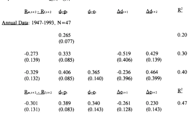
Table 5: Future Dividends, Future Earnings, and Returns
Dependent variable: ~,,+l-R~,l+l b.t+z af,t+2 dt~t dl%t Mt+l Mt+z g Annual Da@:1947-1993, N=47 0.265 0.20 (0.077) -0.273 0.333 -0.519 0.429 0.30 (o. 139) (0.085) (0.406) (0.139) -0.329 0.406 0.365 -0.236 0.464 0.40 (O.132) (0.085) (o. 140) (0.396) (0.399)_R,t+2af,t+2 dlqt dt%t &t+l &t+2 p
-0.301 0.389 0.340 -0.261 0.230 0.47
Table 6: Payout Ratio and Excess Returns on Corporate Bonds
Dependent variable: R~,,+,- R~,,~b,t~,t dt~t dl~, -t DE FAULTL g
QuarterlyData 47Q1 -92Q4, N= 184
AAA COWOate Bowr
-0.014 0.090 (0.074) (0.046) -0.142 0,097 (0.083) (0.058) AA Co@orateBona -0.013 0.088 (0.074) (0.045) -0.153 0.082 (0.083) (0.057)
A Co@o ater Bonds
0.004 0.090 (0.074) (0.046) -0.146 0.084 (0.084) (0.058) BAACOWOatr e Bonds 0.090 0.101 (0,074) (0.047) -0,087 0.085 (0.084) (0.058)
Low Grade CorDorateBonds
0.059 0.167 (0.073) (0.052) -0.033 0.128 (0.077) (0.066) 0.154 (0.082) 0.109 (0.085) 0.155 (0.081) 0.100 (0.083) 0.168 (0.083) 0.112 (0.085) 0.161 (0.084) 0.093 (0.085) 0.283 (0.095) 0.208 (0.097) 0.033 (0.010) 0.035 (0.010) 0.037 (0.011) 0.043 (0.011) 0.035 (0.011) -0.05 (0.054) 0.013 (0.053) 0.018 (0.054) 0.028 (0.054) 0.066 (0.061) 0.03 0,08 0.03 0.09 0.03 0.10 0.05 0.13 0.08 0.14 Quarterly DaM 47 Q1-93Q1, N= 185
s&P Compo site
0.080 0.361 0.327 0.047 -0.020 0.13
(0.071) (0.112) (0.164) (0.018) (o. 104)
Sma11stock
-0.022 0.367 0.193 0.059 -0.032 0.06
(0.073) (0.173) (0.254) (0.027) (0.161)
Notes: TERM is thedifference beLween the AAA Corporatebond rate md the l-month treasurybill rate.
Table 7: Expected Stock Returns and Business Conditions
Dependent variable: ~,,+1 -R~,t Quarterly D~ &,ta,t dt~l 47Q1-94Q4 0.082 0.334 N=192 (0.070) (0.086) k,taf.t dt~t 47Q2-94Q4 0.071 0.341 N=191 (0.072) (0.087) &,taf,t ~t~l 47Q 1-94Q4 0.097 0.306 N=192 (0.070) (0.088) ~,,~f,[ dt~t 47 Q2-94Q4 0.081 0.357 N=191 (0.070) (0.089) Notes: dt+t 0.328 (0. 163) dt+t 0.288 (O.187) di+l 0.410 (O.152) dtat 0.340 (o. 190) M, &t -0.162 -0.159 (0.290) (O.123) ~1 ~f,t -0.756 -0.440 (0.683) (0.866) ~t 0.074 (0.054) Gtit ltflt 0.980 -0,477 (0.598) (0.351) ~z 0.11 R2 0.11 R2 0.11 R2 0.12n, is the annualized CPI inflation rate during quarter t and rf.Lis the three-month t-bill rate at the end of quarter t. RECESSION is a dummy variable equal to one in quarters which are between a business cycle peak and trough, as defined by the National Bureau of Economic Research. cl-y, and it-y, are the (natural logs 00 the consumption to GDP and investment to GDP rat ios, where consumption is real nondurable and services consumption, and investment is real gross fixed private investment.
Table 8: Different Measures of Stock Prices and Corporate Profits
Dependent variable: ~,~+1 - R~,~+l Rmt-Rfl d,~t dtat btflt yt%,,N~A g —)— ! Annua1 Da~ 1947-1991 -0.083 0.357 0.334 -0.019 0.29 N= (0.141) (0.234) (O.167) (o. 155) 45 1947-1991 -0.038 0.372 0.200 0.25 N= (o. 140) (O.167) (0.058) 45 Quar terlv Dm 47Q2-94Q4 0.095 0.405 0.387 N=191 (0.070) (0.091) (0.156) 0.112 0.12 (0.068) 47Q2-94Q4 0.118 0.342 N=191 (0.070) (0.088) 0.140 0.09 (0.068)Notes: bl-m, is the log of the ratio of the book value of the S&P Industrials Index and the price level of the Industrial Index. For quarterly data, B is the level at the end of the previous year, and M is the level at the end of the previous year times the change in the total return index. Y,‘et,NIpA is the log of the ratio of gross domestic product by corporate business to corporate
Table 9: Earnings and Expected Returns, 1947-1994 and 1871-1987
Dependent variable: %,~+1 - Rf,t+l &,t+,t N=192 (0.070) 47Q1-94Q4 0.107 N=192 (0.070) 47Q1-94Q4 0.114 N=192 (0.071) Annual Dau 1876-1987 0.212 N=112 (O.106) 1876-1987 0.207 N=112 (o. 107) 1876-1987 0.211 N=112 (0.101) dt$t 0.348 (0.086) 0.326 (0.085) 0.150 (0.067) 0.158 (0.069) 0.369 0.065 (0.208) (0.220) 0.330 (0.163) 0.421 (o. 190) -0.029 (0.064) 0.172 (0.076) 0.08 0.221 0.06 (0.076) 0.05 0.06 0.163 0.08 (0.062)Notes: e5, is the average of the current and four years past earnings per share. The quarterly data are the same as in Table 3. All annual data from this table are from the data series printed in Shiner (1989). Total return in year t is calculated as ~,~= ln(P~+l+ D~-ln(P~, where Pi is the price level in January of year t+ 1 and D, is dividends paid in year t. The risk-free rate, Rf,,, is constructed using 6-month commercial paper is described in Shiner (1989). The data start in 1871; the sample starts in 1876 to allow lags for computing e5.
Table A: Alternate Measures and Samples
Dependent variable: ~,t+l -Rf,L+l Alternative Measures 1947Q 1-1994Q4 N=192 1947Q1- 1994Q4 N=192 1947Q1- 1994Q4 N=192 1954Q2-1994Q4 N=192 L,(-f,t 0.109 (0.070) 0.086 (0.069) &t-Rfl,— , 0.020 (0.073) L,(af,, 0.131 (0.076) Alternative Samples &,(af,L 1947Q 1-1970Q4 0.105 N=96 (0.101) 1970Q4- 1994Q4 0.105 N=96 (0.101)km
0.356 (0.087) 0.332 (0.079) 4s, 0.354 (0.088) &,RT%,RT 0.546 (0.143) dtal 0.282 (0.097) 0.513 (o. 179) &,NmA&,mA 0.213 (0.082) &.,s.l 0.333 (O.152) ~t.RT&.RT 0.660 (0.231) d+, 0.344 (0.293) 0.578 (0.235) 0.426 0.13 (0.112)0,10
Notes: d-p is the log of the dividend-price ratio of the S&P Composite Index. d,,mA-e,,mA is the log of the ratio of Dividend and Profit After Tax reported in the Department of
Commerce’s National Income and Product Accounts. dt-et,~TRis the log of the ratio of the four-quarter total of dividends reported by S&P to (four times the) single quarter earnings reported by S&P. The single quarter earnings are not seasonal] y adjusted. dt,RT-e~,RTis the “real-time” log dividend payout ratio, constructed by taking using price-earnings and dividend yield observations calculated in real time. d,,R~-eL,~Tis the urea]-time” log dividend yield.
n
-.
—
al L = a)0
.0
C.f)0
0
Ll-r
0
a)0
l-f) 00
m
0
0
> ~ ,. -/ - --.—. _ -, . _—— ---_—— -— --<--’ _-— --- - ---—___ ---—___ - _. _-_= - =-___ _ —----— --- -_-_--_— -_-_- _-_—_— _____ _ _ —-_ - --- ~- ---—-—-—_—_—_ -. ---> -- --L<3_-::::~’”
---‘
:–’~
--- --
,
---- .
--- .-_-” -—-_-—— —--- - -->. --- —-_ _ --l-f) h
0
I I I I IOmou)o
mmu)wr00000
0
3/a
I I I I I 1 I I I i I I I / I / / \ / 1 I \ 1 I \ I I \
,“
\ ,’ \ \,’
\,,’
,i
,j / \ / / \ / \ / \ / / \ / / ) / \ \/’
I I [ f I / I \ I I I I I Im
—
t L L —mm
00
qo
INotes on Figure 2.
The figure shows impulse response functions from a standard vector autoregression on the vector (d-e, d-p, ~-R~), with four quarterly lags, using