On Combination of SMOTE and Particle Swarm Optimization Based
Radial Basis Function Classifier for Imbalanced Problems
Ming Gao, Xia Hong, Sheng Chen and Chris J. Harris
Abstract—The combination of the synthetic minority over-sampling technique (SMOTE) and the radial basis function (RBF) classifier is proposed to deal with classification for imbalanced two-class data. In order to enhance the significance of the small and specific region belonging to the positive class in the decision region, the SMOTE is applied to generate synthetic instances for the positive class to balance the training data set. Based on the over-sampled training data, the RBF classifier is constructed by applying the orthogonal forward selection procedure, in which the classifier structure and the parameters of RBF kernels are determined using a particle swarm opti-mization algorithm based on the criterion of minimizing the leave-one-out misclassification rate. The experimental results on both simulated and real imbalanced data sets are presented to demonstrate the effectiveness of our proposed algorithm.
I. INTRODUCTION
Generally speaking, an imbalanced problem occurs when the instances in one or several classes (the majority classes) outnumber the instances of the other classes (the minority classes), which usually are the more important classes. Such an imbalance in the data represents the so-called between-class imbalance [1], in contrast to the related issue of within-class imbalance [2][3]. Imbalanced problems widely exist in the field of medical diagnosis, such as surveillance of nosocomial infection [4], cardiac care [5] and elucidating protein-protein interactions [6]) as well as in many other fields, such as fraud detection [7][8], network intrusion detection [9], telecommunication management [10], and so on. In the study of two-class imbalanced problem, the instances in the majority class are referred to as negative, while in its counterpart, the minority class, the instances are referred to as positive. Since in practice the minority class is more important, one should be more concerned with the positive instances. Imbalanced data learning has been widely researched [11]-[16]. Typically, the approaches to solving the imbalanced problem can be divided into two categories: re-sampling methods and imbalanced learning algorithms.
The re-sampling approach is actually a re-balancing pro-cess to balance the given imbalanced data set. The studies [17][18] on class distribution have shown that balanced data sets provide better learning performance than imbalanced ones, though some other studies [1][19] argue that imbal-anced data sets are not necessarily responsible for the poor performance of some classifiers. Re-sampling techniques are M. Gao and X. Hong are with the School of Systems Engi-neering, University of Reading, Reading RG6 6AY, UK (E-mails: [email protected]; [email protected]).
S. Chen and C.J. Harris are with the School of Electronics and Computer Science, University of Southampton, Southampton SO17 1BJ, UK (E-mails: [email protected]; [email protected]).
This work was supported by UK EPSRC.
attractive under most imbalanced circumstances. This is be-cause re-sampling adjusts only the original training data set, instead of modifying the learning algorithm. Thus, this ap-proach is external and transportable [18][20], and it provides a convenient and effective way to deal with imbalanced learn-ing problems uslearn-ing standard classifiers. Specifically, the re-sampling methods include the random over-re-sampling, which randomly appends replicated instances to the positive class, and the random under-sampling, which randomly removes instances from the majority class. Alternatively, there exist the guided over-sampling and under-sampling, respectively, of which the choices to replace or to eliminate are informed rather than random. In addition, the synthetic minority over-sampling technique (SMOTE) [21] is a well acknowledged over-sampling method. In the SMOTE, instead of mere data oriented duplicating, the positive class is over-sampled by creating synthetic instances in the feature space formed by the instance and itsK-nearest neighbors.
The second category, the imbalanced learning algorithms, can be regarded as a process to modify or improve the existing learning algorithms so that they can deal with imbalanced problems effectively. The imbalanced learning algorithms include the cost-sensitive method [22]-[25], the discrimination-based and recognition-based approaches [3]. Noticeably, kernel-based learning, such as support vector ma-chine (SVM) and radial basis function (RBF), is the state-of-the-arts approach for solving imbalanced learning problems. The study [1] shows that kernel-based methods provide a relatively robust classification to imbalanced problems. Nev-ertheless, the detrimental effects of an imbalanced data set can be sufficiently serious to prevent kernel-based classifiers from achieving the optimal classifier’s performance.
In order to achieve better classification performance, an effective approach is to integrate kernel-based classifiers with re-sampling methods. The previous studies [26]-[28] mainly focused on SVMs. Specifically, the method [26] combined the SMOTE with different costs to bias SVMs by assigning different classes with different costs so as to shift the decision boundary away from the positive instances and to define a better boundary. The work [27] proposed ensemble systems by re-sampling data sets to form the input to the standard SVM classifier, while the method [28] introduced asymmetric misclassification costs in SVMs so as to improve classification performance. Another integration of SVM with under-sampling method used the combination of the granular support vector machine (GSVM) [29] and repetitive under-sampling (RU) to form the GSVM-RU algorithm [30]. An alternative approach is to adapt kernel-based classifiers to imbalanced data sets by modifying the kernel construction Proceedings of International Joint Conference on Neural Networks, San Jose, California, USA, July 31 – August 5, 2011
and model selection procedure. A representative work of this approach [31] proposed a regularized orthogonal weighted least square (ROWLS) kernel estimator using the orthogonal forward selection (OFS) based on the model selection crite-rion of maximizing the leave-one-out area under the curve (LOO-AUC) of receiver operating characteristics (ROC).
For balanced data sets, the prevalent approach for con-structing the RBF and other sparse kernel classifiers is to assign a fixed common variance for every kernel and to select input data as the candidate centers for RBF kernels by minimizing the leave-one-out (LOO) misclassification rate in the efficient OFS procedure [32]. This approach has its root in regression application [33]-[36]. There are two limitations with this “fixed” RBF kernel approach. Firstly, kernels cannot be flexibly tuned, as the position of each kernel is restricted to the input data and the shape of each kernel is fixed rather than determined by the model learning procedure. Secondly, the common kernel variance has to be determined via cross validation, which inevitably increases the computational cost. The previous studies [37]-[39] constructed the tunable RBF classifier based on the OFS procedure using a global search optimization algorithm [40] to optimize the RBF kernels one by one. This tunable RBF kernel approach was observed to produce sparser classifiers with better performance but higher computational complexity in classifier construction, in com-parison with the standard fixed kernel approach. Recently, the particle swarm optimization (PSO) algorithm [41] was adopted to minimize the LOO misclassification rate in the OFS construction of tunable RBF classifier [42][43]. PSO [41] is an efficient population-based stochastic optimization technique inspired by social behaviour of bird flocks or fish schools, and it has been successfully applied to wide-ranging optimization applications [44]-[48]. Owing to the efficiency of PSO, the tunable RBF modeling approach advocated in [42][43] offers significant advantages in terms of better generalization performance and smaller classifier size as well as lower complexity in learning process, compared with the standard fixed kernel approach. This PSO aided tunable RBF classifier, therefore, offers the state-of-the-art for balanced data sets. When dealing with highly imbalanced problems, however, its performance may degrade.
Against this background, our novel contribution is to combine the SMOTE algorithm and the PSO aided RBF classifier to deal with two-class imbalanced classification problems effectively. The SMOTE is first applied to generate synthetic instances in the positive class to balance the training data set. Using the resulting balanced data set, the tunable RBF classifier is then constructed by applying the PSO to minimize the LOO misclassification rate in the computation-ally efficient OFS procedure. Experimental results obtained demonstrate that the proposed method is competitive to other existing state-of-the-arts methods for two-class imbalanced problems. The rest of the paper is organized as follows. Section II introduces the tunable RBF model for two-class classification and the OFS procedure based on the LOO misclassification rate, while Section III presents the PSO
algorithm for tuning the RBF kernels by minimizing the LOO misclassification rate. Section IV introduces the SMOTE method and presents the proposed combined SMOTE and PSO based RBF algorithm. The effectiveness of our approach is demonstrated by numerical examples in Section V, and our conclusions are given in Section VI.
II. TUNABLERBFMODELING FOR CLASSIFICATION Consider the two-class data setDN ={xk, yk}Nk=1, where
yk = {±1} denotes the class label for the feature vector xk ∈ m, while there are N
+ positive instances and N−
negative instances, withN =N++N−. We use the data set
DN to construct the RBF classifier of the form: ˆ yk(M)=M i=1wigi xk=gT M(k)wM ˜ yk(M)=sgnyˆk(M) (1)
whereM is the number of RBF kernels,yˆ(kM) is the output of the M-term classifier with theM kernels,gi(•)for1≤ i≤M, andy˜(kM) denotes the corresponding estimated class label forxk, while wM =
w1 w2· · ·wM T is the weight vector and gMT(k) = g1(xk) g2(xk)· · ·gM(xk) . In this study, we use the Gaussian kernel function
gi(x) = exp −(x−ci)TΣ−1 i (x−ci) (2) whereci∈ mis the center vector of theith RBF kernel and Σi =diag{σi,21, σ2i,2,· · ·, σ2i,m} is the diagonal covariance matrix of theith kernel. Hence, the position of each kernel, ci, and coverage of each kernel, Σi, are both considered as
the parameters to be determined in kernel modeling. From (1), the RBF classifier over DN can be written in
the matrix form as
y=GMwM +e(M) (3) where e(M) = e(M)
1 e(2M)· · ·e(NM)
T
is the error vector with the M-term modeling error e(kM) = yk − yˆ(kM), y = y1 y2· · ·yNT is the desired class label vector, and the kernel matrix GM =
g1 g2· · ·gM with gl =
gl(x1)gl(x2)· · ·gl(xN)
T
for1≤l≤M. Note thatgl is
thelth column ofGM whilegMT(k)is thekth row ofGM.
Consider the orthogonal decompositionGM =PMAM,
where AM = ⎡ ⎢ ⎢ ⎢ ⎢ ⎣ 1 a1,2 · · · a1,M 0 1 . .. ... .. . . .. ... aM−1,M 0 · · · 0 1 ⎤ ⎥ ⎥ ⎥ ⎥ ⎦ (4) PM =p1 p2· · ·pM (5) and the columns in (5) satisfypTi pj = 0fori=j. The RBF
classifier (3) can alternatively be represented as:
y=PMθM +e(M) (6)
whereθM =
θ1 θ2· · ·θMTsatisfies θM =AMwM. The
space spanned by the original model basesgi,1≤i≤M,
The OFS procedure constructs the RBF kernels one by one by minimizing the LOO misclassification rate [42][43]. Specifically, at thenth stage, thenth RBF kernel (pnandθn)
is determined. Define the LOO-model output of then-term RBF model constructed from the LOO data setDN\(xk, yk),
calculated at xk, as yˆ(kn,−k). Further define the associated
LOO decision variable as
sk(n,−k)=sgn(yk)ˆyk(n,−k)=ykyˆk(n,−k) (7)
Then the LOO misclassification rate is defined by [32]
JLOO(n) = 1 N N k=1 Id s(kn,−k) (8) in which the indicator functionId(s)is defined as
Id(s) =
1
, s≤0
0, s >0 (9)
By making use of Sherman-Morrison-Woodbury theorem [49] as well as the orthogonal property, the LOO de-cision variable can be efficiently calculated according to [32][42][43]
s(kn,−k)= ψ
(n)
k
ηk(n) (10)
in whichψk(n)andη(kn) can be computed recursively by:
ψ(kn)=ψk(n−1)+ykθnpn(k)− p2n(k) pT npn+λ (11) ηk(n)=η(kn−1)− p 2 n(k) pT npn+λ (12) wherepn(k)is thekth element ofpn andλ≥0 is a small
regularization parameter.
At the nth stage of the OFS procedure, the nth RBF kernel, namely, its center vectorcn and diagonal covariance
matrix Σn, are determined by minimizing JLOO(n) . The
con-struction terminates at the size ofM whenJLOO(M+1)≥JLOO(M)
[32][42][43].
III. PSOFOR OPTIMIZINGRBFPARAMETERS Let μ= [μ(1) μ(2)· · ·μ(2m)]T be the 2m-dimensional vector that contains cn and Σn. Then, as defined in the
previous section, the problem of determining the nth RBF kernel’s parameters at the nth OFS stage is to solve the following optimization problem
ˆ
μ= arg min
μ∈ΓJ (n)
LOO (13)
where Γ defines the 2m-dimensional search space for the parameter vector μ, which is specified by the two val-ues Γmin = Γ1,min Γ2,min· · ·Γ2m,minT and Γmax =
Γ1,max Γ2,max· · ·Γ2m,maxT as follows. The search space forcn=
cn,1cn,2· · ·cn,m
T
is specified by the distribution of the training data xk =
xk,1 xk,2· · ·xk,m
TN k=1, namely,
cn,i∈xmin,i, xmax,iΓi,min, Γi,max,1≤i≤m (14)
with xmin,i = min
1≤k≤Nxk,i andxmax,i = max1≤k≤Nxk,i, while
each element ofΣn is limited in the range σn,i2 ∈ σ2min, σ2max
Γ(i+m),min, Γ(i+m),max, 1≤i≤m (15) When applying a PSO [41] to solve the optimisation (13), a swarm of the candidate particles μ[il]Si=1 are “flying” in the search space Γ in order to find a solution μˆ, where
S is the size of the swarm and l ∈ {0,1,· · ·, L} denotes the lth movement of the swarm. Each particle μ has a
2m-dimensional velocity ν = [ν(1) ν(2)· · ·ν(2m)]T to direct its search, and the velocityν ∈ V with the velocity space defined by V =−Vmax, Vmax, where Vmax =
V1,max V2,max· · ·V2m,maxT= 12Γmax−Γmin.
To start the PSO, the candidate particles μ[0]i Si=1 are initialized randomly withinΓ, and the velocity for each can-didate particle is initialized to zero, namely,ν[0]i =0Si=1. The cognitive information pb[il] and the social information gb[l]record the best position visited by the particleiand the best position visited by the entire swarm, respectively, during the l movements. For notational convenience, we denote the LOO cost calculated on pb[il] as JLOO(n) pb[il] and the LOO cost calculated ongb[l] as JLOO(n) gb[l]. The cognitive information pb[il] and the social information gb[l] are used to update the velocities and positions according to
ν[l+1] i = a·ν [l] i +rand()·b· pb[l] i −μ [l] i +rand()·c·gb[l]−μ[il] (16) μ[l+1] i = μ[ l] i +ν[ l+1] i (17)
where a denotes the inertia weight, rand() is the random number uniformly distributed in [0, 1],b andc are the two acceleration coefficients. Experimental results given in [43] show that a better performance can be achieved by using
a =rand() instead of a constant inertia weight. Adopting the time varying acceleration coefficients (TVAC) [44], in whichb= 2.5−(2.5−0.5)·l/Landc= 0.5 + (2.5−0.5)· l/L, can often enhance the performance of PSO. The search spaceΓand the velocity spaceVare used to confineμ[il+1] andν[il+1] derived from (16) and (17), respectively. Ifν[il+1] becomes too close to0, a random re-initialization is needed, which may take the formν[il+1]=±0.1·rand()·Vmax. The
detailed PSO aided OFS algorithm can be found in [43]. IV. COMBINEDSMOTEANDPSOOPTIMIZEDRBFFOR
IMBALANCED CLASSIFICATION
The SMOTE [21] over-samples the positive class by creat-ing synthetic instances by a specified over-samplcreat-ing ratio of the original minority data size,β%. Based on each minority data sample, denoted by xo, β% synthetic data points are
generated by randomly selecting data points on the lines linkingxowith some of itsKnearest neighbors, whereKis
predetermined. Depending on the required SMOTE amount
β%, one out of theKnearest positive class data samples are randomly selected several times. For example, ifβ% = 600%
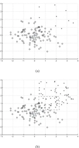
−3 −2 −1 0 1 2 3 4 −3 −2 −1 0 1 2 3 4 (a) −3 −2 −1 0 1 2 3 4 −3 −2 −1 0 1 2 3 4 (b)
Fig. 1. (a) Original training data space, and (b) training data space after SMOTE over-sampling the positive class by 500% of its original size, where x denotes positive class instance while◦denotes negative class instance
and K = 5, then one out of five nearest neighbors of xo
is randomly chosen repeatedly for six times. Each time a randomkth neighbor is selected to create a line linkingxoto
this neighbor, and then a single synthetic instance is created by randomly selecting a point on the line. Thus any synthetic instancexs is given by
xs=xo+δ·x{ot}−xo
(18) where xs denotes one synthetic instance, x{ot} is the tth
nearest neighbors ofxo in the positive class, andδ∈[0, 1]
is a random number. The procedure is repeated for all the positive data points.
A major problem caused by imbalanced data sets is that most classifiers tend to attribute the positive class instances within the decision region to the negative class, due to insufficient positive-class training instances in the decision region. As a result, the trained decision boundary tends to be far away from the negative class and too close to the positive class. The contribution of SMOTE is to enhance the significance of the small and specific region belonging to the positive class in the decision region, which leads to the better generalization for classifiers. Fig. 1(a) shows a simulated imbalanced data set, the details of which are specified in Section V. After the SMOTE over-sampling the positive class by 500% of its original size, the instances from the positive
class become more significant in the decision region (the area specified by dash-dot line), as shown in Fig. 1(b), compared with the original data set. Consequently, the trained decision boundary tends to be further away from the positive class.
We combine this SMOTE with the PSO optimized RBF classifier described in Section III to create a powerful al-gorithm for combating two-class imbalanced problems. This combined SMOTE and PSO aided RBF is detailed below.
1) Algorithm initialization
(a) Specify the balanced degreeβ%and the value ofK. Create the new training data setD˜N by appending the generated positive training data points to the original training data set via the SMOTE.
(b) Specify the search spaceΓ and the velocity space V. Specify the values of LandS.
(c) SetJLOO(0) = 1,ψk(0)= 0, andηk(0)= 1. 2) Construct thenth RBF kernel
(a) PSO initialization: Randomly initialize {μ[0]i }S i=1 inΓ, and set {ν[0]i =0}S
i=1. (b) For 0≤l < L:
(b.i) Construct the candidates g{ni} fromμ[il], for 1≤ i≤S. Then, for 1≤i≤S and1≤j < n, compute:
a{j,ni} = 1 , n= 1 pT jg{ni} pT jpj , n >1 p{i} n = ⎧ ⎪ ⎨ ⎪ ⎩ g{i} n , n= 1 g{i} n − n−1 j=1a {i} j,npj, n >1 θn{i}= p{i} n T y p{ni} T p{ni}+λ
(b.ii) For1≤i≤S and1≤k≤N, compute:
ψ(kn){i}=ψ(kn−1)+y(k)θn{i}p{ni}(k)− p{ni}(k) 2 p{i} n T p{i} n +λ η(kn){i}=ηk(n−1)− p{ni}(k) 2 p{ni} T p{ni}+λ
Then, for 1≤i≤S, calculate the LOO costs:
JLOO(n) {i}= N1 N k=1Id ψk(n){i} ηk(n){i} (b.iii) For1≤i≤S:
If JLOO(n) {i} < JLOO(n) pbi[l]: pb[il] = μ[il] and
JLOO(n) pbi[l]=JLOO(n) {i}
Then find i∗= arg min
1≤i≤SJ (n) LOO pb[l] i
If JLOO(n) pbi[l∗] < JLOO(n) gb[l]: gb[l] = pb[il∗] and
JLOO(n) gb[l]=JLOO(n) pb[il] ∗ (b.iv) For1≤i≤S: ν[l+1] i = a · ν [l] i + rand() · b · pb[l] i − μ [l] i +rand()·c·gb[l]−μ[il] Ifνi[l+1](j) = 0: νi[l+1](j) =±0.1·rand()·Vj,max Ifνi[l+1](j)> Vj,max:νi[l+1](j) =Vj,max Ifνi[l+1](j)<−Vj,max: νi[l+1](j) =−Vj,max Then for1≤i≤S: μ[l+1] i =μ[ l] i +ν[ l+1] i Ifμ[il+1](j)>Γj,max:μ[il+1](j) = Γj,max Ifμ[il+1](j)<Γj,min:μ[il+1](j) = Γj,min
(c) Termination of PSO: gb[L] provides cn and Σn
with the associated LOO costJLOO(n) =JLOO(n) gb[L]. The algorithm also generates aj,n for1≤j < n,pn
andθn as well as ψk(n) andηk(n) for1≤k≤N.
3) OFS termination condition checking:
IfJLOO(n) < JLOO(n−1):n=n+ 1, go to step 2);
Otherwise, M =n−1, terminate the OFS procedure. V. EXPERIMENTAL RESULTS
The effectiveness of the proposed SMOTE+PSO-OFS al-gorithm was investigated using a simulated imbalanced date set and three real imbalanced data sets. The first two real data sets were taken from [50], while the third real data set was from [51]. These three real data sets were chosen in the order of increasing imbalance. For each data set, the positive class was over-sampled at different rates β% of its original size using the SMOTE. For the synthetic data set, a separate test data set was used, while for the three real data sets,P-fold cross validation was used, to indicate the classifier generalization capability based on multiple specifications, including the true positive rate (TP%) and the false positive rate (FP%) [52], as well as the precision (Pr), the F-measure (F-meas) and the G-mean [53]. These criteria are commonly adopted as the performance metrics for eval-uating imbalanced learning classifiers. The regularized least square parameter estimator (KRLS), theK¯-nearest neighbor classifiers withK¯ = 1and3(1−N Nand3−N N), as well as the LOO-AUC+OFS with different weight ρ were cited from [31] as the benchmarks for comparison in the synthetic and first two real data sets. For the third real data set, the weighted SVM with (C+ = 1000, C−=−1000), the cost sensitive SVM (CS-SVM) with(C+ = 1, C−=−0.1), the cost sensitive SUPANOVA with(C+ = 1, C−=−0.1)and the LOO-AUC+OFS with different weight ρ were quoted from [31][51] as comparison.
Simulated imbalanced data set: The simulated data set was generated with the m = 2 features. The mean vector of the negative class was [0 0]T, while the mean vector of the positive class was[2 2]T. The covariance matrices of both the negative-class and positive-class instances were the same 2-dimensional identity matrix. The training data set contained 100 instances from the negative class and 10 instances from the positive class, as depicted in Fig. 1(a). The test data set contained 1000 instances from the negative class, and 100 instances from the positive class. The 5-nearest neighbor method was applied to generate synthetic training data in the SMOTE, with the over-sampling rate β% set to 0%,
100%,500%,1000%,1500%and2000%, respectively. For the SMOTE+PSO-OFS, the swarm size and the number of movements were set toS= 10andL= 20. The test results obtained by the various classifiers are shown in Table I.
It can be seen from the results for the SMOTE+PSO-OFS listed in Table I that, as the over-sampling rateβ%increases, typically TP% increases but FP% inevitably increases as well. A better tradeoff between TP% and FP% was achieved, however, at the over-sampling rate where the better G-mean
TABLE I
TEST CLASSIFICATION PERFORMANCE COMPARISON FOR THE SYNTHETIC DATA SET
Method TP% FP% Pr G-mean F-meas KRLS with all 0.840 0.037 0.694 0.899 0.760 data as centers 1-NN 0.830 0.047 0.638 0.899 0.722 3-NN 0.780 0.022 0.780 0.873 0.780 LOO-AUC+OFS 0.860 0.049 0.637 0.904 0.732 (ρ= 1) LOO-AUC+OFS 0.840 0.028 0.750 0.903 0.792 (ρ= 5) LOO-AUC+OFS 0.90 0.063 0.588 0.918 0.712 (ρ= 10) LOO-AUC+OFS 0.870 0.046 0.654 0.911 0.747 (ρ= 15) LOO-AUC+OFS 0.870 0.049 0.640 0.909 0.737 (ρ= 20) SMOTE+PSO-OFS 0.860 0.044 0.662 0.907 0.748 (β% = 0%) SMOTE+PSO-OFS 0.880 0.055 0.615 0.912 0.724 (β% = 100%) SMOTE+PSO-OFS 0.810 0.023 0.780 0.890 0.794 (β% = 500%) SMOTE+PSO-OFS 0.890 0.053 0.627 0.918 0.736 (β% = 1000%) SMOTE+PSO-OFS 0.930 0.102 0.476 0.914 0.631 (β% = 1500%) SMOTE+PSO-OFS 0.940 0.110 0.461 0.915 0.618 (β% = 2000%)
and F-measure were obtained. Since the imbalance degree of the negative class to the positive class was 10 : 1, the over-sampled positive instances madeD˜N fully balanced at β% = 1000%. From Table I, it can be seen that the best test performance occurred at the over sampling rate around
500%to1000%. The effect of the SMOTE on the decision boundary is shown in Fig. 2, where it can be seen that the decision boundary trained by the more balanced data set was pushed further away from the positive class. Compared with the other benchmark methods, the proposed SMOTE+PSO-OFS showed a competitive performance.
Pima Indians diabetes data set [50]: The data set con-tained 768 instances from the two classes with 500 negative instances and 268 positive instances. The feature space dimension was m = 8. All the eight input features were normalized to the range[0, 1]using the operation
¯ xk,i=
xk,i−xmin,i
xmax,i−xmin,i, 1≤k≤N,1≤i≤m (19)
The 5-nearest neighbor scheme was applied to generate synthetic training data in the SMOTE. The over-sampling rate
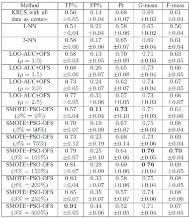
β% was set to 0%, 50%, 75%,100%,150%,200%, 250% and500%, respectively. The swarm size and the number of movements were set to S = 10and L = 20 for the PSO. The 8-fold cross validation was used to investigate the test performance of a classifier. The8-fold cross validation results for the various classifiers are shown in Table II.
For the SMOTE+PSO-OFS, it can be seen that the best TP%, that is, the best detection capability for diabetes, occurred at β% = 500%, while the best FP% occurred at
β% = 0%. But the best TP% was obtained at the expense of the worst FP%, and the best FP% was obtained at the expense of the worst TP%, as indicated by the poor values of the
G-−3 −2 −1 0 1 2 3 4 5 −4 −3 −2 −1 0 1 2 3 4 5 6 (a) −3 −2 −1 0 1 2 3 4 5 −4 −3 −2 −1 0 1 2 3 4 5 6 (b) −3 −2 −1 0 1 2 3 4 5 −4 −3 −2 −1 0 1 2 3 4 5 6 (c) −3 −2 −1 0 1 2 3 4 5 −4 −3 −2 −1 0 1 2 3 4 5 6 (d)
Fig. 2. Decision boundaries obtained by the SMOTE+PSO-OFS with different over-sampling rates: (a)β% = 0%, (b)β% = 100%, (c)β% = 1000%, and (d)β% = 2000%, where x denotes positive-class test instance while◦denotes negative-class test instance.
TABLE II
8-FOLD CROSS VALIDATION CLASSIFICATION PERFORMANCE FORPIMA
INDIANS DIABETES DATA SET
Method TP% FP% Pr G-mean F-meas KRLS with all 0.56 0.14 0.68 0.69 0.61 data as centers ±0.05 ±0.04 ±0.07 ±0.03 ±0.04 1-NN 0.54 0.21 0.58 0.65 0.56 ±0.04 ±0.04 ±0.06 ±0.02 ±0.04 3-NN 0.58 0.17 0.65 0.69 0.61 ±0.06 ±0.06 ±0.07 ±0.04 ±0.04 LOO-AUC+OFS 0.58 0.13 0.70 0.71 0.63 (ρ= 1.0) ±0.03 ±0.05 ±0.09 ±0.03 ±0.05 LOO-AUC+OFS 0.68 0.20 0.65 0.73 0.66 (ρ= 1.5) ±0.06 ±0.07 ±0.08 ±0.04 ±0.05 LOO-AUC+OFS 0.73 0.24 0.62 0.74 0.67 (ρ= 2.0) ±0.05 ±0.07 ±0.07 ±0.04 ±0.05 LOO-AUC+OFS 0.77 0.31 0.57 0.73 0.66 (ρ= 2.5) ±0.05 ±0.06 ±0.05 ±0.03 ±0.07 SMOTE+PSO-OFS 0.57 0.11 0.73 0.71 0.64 (β% = 0%) ±0.04 ±0.04 ±0.10 ±0.03 ±0.06 SMOTE+PSO-OFS 0.70 0.19 0.67 0.75 0.68 (β% = 50%) ±0.07 ±0.09 ±0.07 ±0.03 ±0.04 SMOTE+PSO-OFS 0.73 0.23 0.68 0.73 0.69 (β% = 75%) ±0.12 ±0.19 ±0.14 ±0.06 ±0.04 SMOTE+PSO-OFS 0.79 0.25 0.64 0.76 0.70 (β% = 100%) ±0.07 ±0.10 ±0.06 ±0.05 ±0.04 SMOTE+PSO-OFS 0.81 0.29 0.60 0.76 0.69 (β% = 150%) ±0.07 ±0.09 ±0.06 ±0.04 ±0.05 SMOTE+PSO-OFS 0.83 0.33 0.58 0.75 0.68 (β% = 200%) ±0.04 ±0.07 ±0.06 ±0.04 ±0.05 SMOTE+PSO-OFS 0.85 0.35 0.57 0.74 0.68 (β% = 250%) ±0.07 ±0.07 ±0.07 ±0.06 ±0.06 SMOTE+PSO-OFS 0.91 0.44 0.52 0.71 0.67 (β% = 500%) ±0.05 ±0.06 ±0.05 ±0.04 ±0.05
mean and F-measure. The best tradeoff between TP% and FP% occurred around β% = 100%to = 150%, which en-abled to detect as many positive diabetes patients as possible while ensuring the minimum incorrect diagnose of healthy people. Again, this best over-sampling rate made the enlarged data set fully balanced. The results of Table II also show that the test performance of the proposed SMOTE+PSO-OFS compare favourably with the other classifiers.
Haberman survival data set [50]: The data set contained 306 instances from the two classes with 225 negative in-stances and 81 positive inin-stances. The feature space dimen-sion wasm= 3. All the three input features were normalized to the range[0, 1]using the operation (19). The 5-nearest neighbor method was adopted to generate synthetic training data in the SMOTE. The over-sampling rateβ% was set to
0%,100%,200%,300%and400%, respectively. The swarm size and the number of movements were chosen to beS= 10
andL= 20. The3-fold cross validation was used to calculate test performance, and the results obtained for the various classifiers are shown in Table III. Compared with the other benchmark classifiers, the SMOTE+PSO-OFS demonstrated its competitive performance. For the SMOTE+PSO-OFS, the best tradeoff between TP% and FP% occurred around
β% = 150%, which was again close to the imbalanced degree of the original data set.
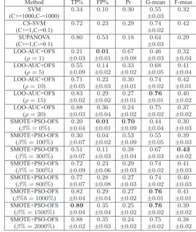
ADI data set: The austempered ductile iron (ADI) material data set was obtained from a study on fatigue cracks from the graphite nodules within the microstructure in an automotive camshaft application [51]. This two-class data set contained
TABLE III
3-FOLD CROSS VALIDATION CLASSIFICATION PERFORMANCE FOR
HABERMAN SURVIVAL DATA SET
Method TP% FP% Pr G-mean F-meas KRLS with all 0.33 0.11 0.63 0.54 0.41 data as centers ±0.05 ±0.01 ±0.07 ±0.04 ±0.05 1-NN 0.32 0.21 0.36 0.50 0.38 ±0.03 ±0.02 ±0.01 ±0.02 ±0.02 3-NN 0.17 0.15 0.30 0.38 0.22 ±0.06 ±0.06 ±0.07 ±0.04 ±0.04 LOO-AUC+OFS 0.21 0.05 0.61 0.45 0.31 (ρ= 1) ±0.02 ±0.01 ±0.05 ±0.02 ±0.03 LOO-AUC+OFS 0.38 0.13 0.51 0.57 0.44 (ρ= 2) ±0.08 ±0.02 ±0.02 ±0.05 ±0.06 LOO-AUC+OFS 0.62 0.27 0.45 0.67 0.52 (ρ= 3) ±0.08 ±0.03 ±0.05 ±0.05 ±0.06 LOO-AUC+OFS 0.67 0.42 0.36 0.62 0.47 (ρ= 4) ±0.02 ±0.08 ±0.03 ±0.03 ±0.02 SMOTE+PSO-OFS 0.23 0.07 0.57 0.44 0.31 (β% = 0%) ±0.04 ±0.06 ±0.01 ±0.05 ±0.05 SMOTE+PSO-OFS 0.44 0.15 0.52 0.61 0.48 (β% = 100%) ±0.09 ±0.06 ±0.09 ±0.07 ±0.09 SMOTE+PSO-OFS 0.63 0.23 0.50 0.69 0.55 (β% = 200%) ±0.06 ±0.06 ±0.07 ±0.08 ±0.09 SMOTE+PSO-OFS 0.80 0.58 0.34 0.57 0.47 (β% = 300%) ±0.09 ±0.07 ±0.05 ±0.09 ±0.05 SMOTE+PSO-OFS 0.84 0.69 0.31 0.51 0.45 (β% = 400%) ±0.08 ±0.08 ±0.04 ±0.08 ±0.05
2923 instances in the feature space of dimension m = 9, with 2807 negative instances and 116 positive instances. As in [31][51], 700 negative-class instances and 90 positive-class instances were randomly selected from the original data set to form the 8-fold cross validation set. Initially, all the nine input features were normalized to within the range [0, 1]
using the operation (19). The SMOTE adopted the5-nearest neighbor scheme to generate synthetic training data. The over-sampling rateβ%was set to0%,100%,300%,500%,
800%,1000%,1500%and2000%, respectively. The swarm size and the number of movements were set toS = 10and
L = 20 for the PSO. The 8-fold cross validation results obtained by the various classifiers are shown in Table IV. For the SMOTE+PSO-OFS, the best overall test performance was achieved at the over sampling rate of β% = 1500%, which is competitive to the performance of the CS-SVM, the SUPANOVA and the best LOO-AUC+OFS(ρ= 15).
VI. CONCLUSIONS
The RBF classifier performs well on balanced or slightly imbalanced data sets, and our previous work has provided an efficient and tunable RBF classifier optimized by the PSO. For highly imbalanced data sets, however, the performance of the tunable RBF classifier may no longer be satisfactory. In order to combat challenging imbalanced classification problems, many approaches have been proposed, which aim to reduce the influence from the underlying imbalanced dis-tribution. In particular, the SMOTE is effective to increase the significance of the positive class in the decision region. In this contribution, we have proposed a powerful and efficient al-gorithm for solving two-class imbalanced problems, referred to as the SMOTE+PSO-RBF, by combining the SMOTE and the PSO optimized RBF classifier. The experimental results presented in this study have demonstrated that the
TABLE IV
8-FOLDCROSSVALIDATIONCLASSIFICATIONPERFORMANCE FORADI
DATA SET
Method TP% FP% Pr G-mean F-meas SVM 0.34 0.10 0.30 0.55 0.32 (C+=1000,C-=1000) ±0.03 CS-SVM 0.72 0.23 0.29 0.74 0.42 (C+=1,C-=0.1) ±0.02 SUPANOVA 0.80 0.53 0.18 0.64 0.29 (C+=1,C-=0.1) ±0.03 LOO-AUC+OFS 0.21 0.01 0.67 0.46 0.32 (ρ= 1) ±0.03 ±0.01 ±0.08 ±0.03 ±0.04 LOO-AUC+OFS 0.55 0.14 0.33 0.68 0.41 (ρ= 5) ±0.09 ±0.02 ±0.02 ±0.05 ±0.04 LOO-AUC+OFS 0.71 0.22 0.30 0.74 0.42 (ρ= 10) ±0.05 ±0.03 ±0.01 ±0.02 ±0.01 LOO-AUC+OFS 0.83 0.29 0.27 0.76 0.40 (ρ= 15) ±0.02 ±0.02 ±0.01 ±0.01 ±0.02 LOO-AUC+OFS 0.88 0.36 0.24 0.75 0.37 (ρ= 20) ±0.03 ±0.04 ±0.02 ±0.02 ±0.02 SMOTE+PSO-OFS 0.20 0.01 0.70 0.44 0.30 (β% = 0%) ±0.04 ±0.01 ±0.09 ±0.04 ±0.03 SMOTE+PSO-OFS 0.30 0.04 0.53 0.55 0.39 (β% = 100%) ±0.07 ±0.02 ±0.09 ±0.05 ±0.03 SMOTE+PSO-OFS 0.51 0.11 0.38 0.67 0.43 (β% = 300%) ±0.07 ±0.03 ±0.04 ±0.03 ±0.02 SMOTE+PSO-OFS 0.72 0.23 0.29 0.74 0.41 (β% = 500%) ±0.09 ±0.06 ±0.03 ±0.02 ±0.03 SMOTE+PSO-OFS 0.77 0.28 0.27 0.74 0.40 (β% = 800%) ±0.07 ±0.08 ±0.03 ±0.02 ±0.03 SMOTE+PSO-OFS 0.82 0.29 0.27 0.76 0.41 (β%b= 1000%) ±0.04 ±0.04 ±0.02 ±0.01 ±0.01 SMOTE+PSO-OFS 0.89 0.35 0.25 0.76 0.39 (β% = 1500%) ±0.04 ±0.04 ±0.02 ±0.02 ±0.02 SMOTE+PSO-OFS 0.88 0.35 0.24 0.75 0.38 (β% = 2000%) ±0.02 ±0.03 ±0.02 ±0.02 ±0.02
proposed SMOTE+PSO-RBF offers a very competitive solu-tion to other existing state-of-the-arts methods for combating imbalanced classification problems.
REFERENCES
[1] N. Japkowicz and S. Stephen, “The class imbalance problem: A systematic study,” Intelligence Data Analysis, vol. 6, no. 5, pp. 429– 449, 2002.
[2] G. M. Weiss, “Mining with rarity: A unifying framework,” ACM SIGKDD Explorations Newsletter, vol. 6, no. 1, pp. 7–19, 2004. [3] N. Japkowicz, “Concept-learning in the presence of between-class
and within-class imbalances,” in Advances in Artificial Intelligence, E. Stroulia and S. Matwin, Eds., vol. 2056, pp. 67–77. Springer-Verlag: Berlin, 2001.
[4] G. Cohen, M. Hilario, H. Sax, S. Hugonnet, and A. Geissbuhler, “Learning from imbalanced data in surveillance of nosocomial infec-tion,” Artificial Intelligence in Medicine, vol. 37, pp. 7–18, 2006. [5] R. B. Rao, S. Krishnan, and R. S. Niculescu, “Data mining for
improved cardiac care,” ACM SIGKDD Explorations Newsletter, vol. 8, no. 1, pp. 3–10, 2006.
[6] C. Yu, L. Chou, and D. Chang, “Predicting protein-protein interactions in unbalanced data using the primary structure of proteins,” BMC Bioinformatics, vol. 11, no. 1, pp. 167–177, 2010.
[7] F. Provost, T. Fawcett, and R. Kohavi, “The case against accuracy estimation for comparing induction algorithms,” in Proc. 15th Int. Conf. Machine Learning(Madison, USA), July 24-27, 1998, pp. 445– 453.
[8] T. Fawcett and F. Provost, “Adaptive fraud detection,” Data Mining and Knowledge Discovery, vol. 1, pp. 291–316, 1997.
[9] D. A. Cieslak, N. V. Chawla, and A. Striegel, “Combating imbalance in network intrusion datasets,” inProc. 2006 IEEE Int. Conf. Granular Computing(Atlanta, USA), May 10-12, 2006, pp. 732–737. [10] G. M. Weiss and H. Hirsh, “Learning to predict rare events in event
squences,” in Proc. 4th Int. Conf. Knowledge Discovery and Data Mining(New York, USA), Aug. 27-31, 1998, pp. 359–363.
[11] F. Provost, “Machine learning from imbalanced data sets 101,” AAAI Workshop on Learning from Imbalanced Data Sets, 2000.
[12] H. He and A. Garcia, “Learning from imbalanced data,”IEEE Trans. Knowledge and Data Engineering, vol. 21, no. 9, pp. 1263–1284, 2009.
[13] R. Barandela, J. S. S´anchez, V. Garc´ıa, and E. Rangel, “Strategies for learning in class imbalance problems,” Pattern Recognition, vol. 36, pp. 849–851, 2003.
[14] V. Garc´ıa, J. S. S´anchez, R. A. Mollineda, R. Alejo, and J. M. Sotoca, “The class imbalance problem in pattern classification and learning,” inII Congreso Espa˜nol de Inform´atica, 2007, pp. 283–291. [15] N. V. Chawla, D. A. Cieslak, L. O. Hall, and A. Joshi, “Automatically
countering imbalance and its empirical relationship to cost,”Data Min. Knowl. Discov., vol. 17, no. 2, pp. 225–252, 2008.
[16] G. M. Weiss, K. McCarthy, and B. Zabar, “Cost-sensitive learning vs. sampling: Which is best for handling unbalanced classes with unequal error costs?,” inProc. 2007 Int. Conf. Data Mining, 2007, pp. 35–41. [17] G. M. Weiss and F. Provost, “Learning when training data are costly: The effect of class distribution on tree induction,”Artificial Intelligence Research, vol. 19, pp. 315–354, 2003.
[18] A. Estabrooks, T. Jo, and N. Japkowicz, “A multiple resampling method for learning from imbalanced data sets,” J. Chemical Infor-mation and Modeling, vol. 20, no. 1, pp. 18–36, 2004.
[19] G. E. A. P. A. Batista, R. C. Prati, and M. C. Monard, “A study of the behavior of several methods for balancing machine learning training data,”SIGKDD Exploration Newsletter, vol. 6, no. 1, pp. 20–29, 2004. [20] C. Drummond and R. C. Holte, “C4.5, class imbalance, and cost sensitivity: Why under-sampling beats over-sampling,” in2003 Int. Conf. Machine Learning – Workshop Learning from Imbalanced Datasets II(Washington DC, USA), Aug. 21, 2003, pp. 1–8. [21] N. V. Chawla, K. W. Bowyer, and L. O. Hall, “Smote: Synthetic
minority over-sampling technique,” J. Artificial Intelligence Research, vol. 16, pp. 321–357, 2002.
[22] C. Elkan, “The foundations of cost-sensitive learning,” inProc. 17th Int. Joint Conf. Artificial Intelligence(Seattle, USA), Aug. 4-10, 2001, pp. 973–978.
[23] K. M. Ting, “An instance-weighting method to induce cost-sensitive trees,”IEEE Trans. Knowledge and Data Engineering, vol. 14, no. 3, pp. 659–665, 2002.
[24] M. A. Maloof, “Learning when data sets are imbalanced and when costs are unequal and unknown,” in2003 Int. Conf. Machine Learning – Workshop Learning from Imbalanced Datasets II(Washington DC, USA), Aug. 21, 2003, pp. 1–8.
[25] K. McCarthy, B. Zabar, and G. Weiss, “Does cost-sensitive learning beat sampling for classifying rare classes?” inProc. 1st Int. Workshop Utility-Based Data Mining(Chicago, USA), Aug. 21, 2005, pp. 69–77. [26] R. Akbani, S. Kwek, and N. Japkowicz, “Applying support vector machines to imbalanced datasets,” in Proc. 15th European Conf. Machine Learning(Pisa, Italy), Sept. 20-24, 2004, pp. 39–50. [27] P. Kang and S. Cho, “Eus svms: Ensemble of under-sampled svms for
data imbalance problems,” inProc. 13th Int. Conf. Neural Information Processing(Hong Kong, China), Oct. 3-6, 2006, pp. 837–846. [28] B. X. Wang and N. Japkowicz, “Boosting support vector machines
for imbalanced data sets,” inProc. 17th Int. Conf. Foundations of Intelligent Systems(Toronto, Canada), May 20-23, 2008, pp. 38–47. [29] Y. Tang, Y.-Q. Zhang, Z. Huang, and X. Hu, “Granular svm-rfe
gene selection algorithm for reliable prostate cancer classification on microarray expression data,” inProc. 5th IEEE Symp. Bioinformatics and Bioengineering (Minneapolis, USA), Oct. 19-21, 2005, pp. 290– 293.
[30] Y. Tang and Y.-Q. Zhang, “Granular svm with repetitive undersampling for highly imbalanced protein homology prediction,” inProc. 2006 IEEE Int. Conf. Granular Computing (Atlanta, USA), May 10-12, 2006, pp. 457–460.
[31] X. Hong, S. Chen, and C. J. Harris, “A kernel-based two-class classifier for imbalanced data sets,”IEEE Trans. Neural Networks, vol. 18, no. 1, pp. 28–41, 2007.
[32] X. Hong, S. Chen, and C. J. Harris, “A fast linear-in-the-parameters classifier construction algorithm using orthogonal forward selection to minimize leave-one-out misclassification rate,”Int. J. Systems Science, vol. 39, no. 2, pp. 119–25, 2008.
[33] S. Chen, C. F. N. Cowan, and P. M. Grant, “Orthogonal least squares learning algorithm for radial basis function networks,” IEEE Trans. Neural Networks, vol. 2, no. 2, pp. 302–309, 1991.
[34] X. Hong, P. M. Sharkey, and K. Warwick, “Automatic nonlinear predictive model construction using forward regression and the press statistic,” IEE Proc. Control Theory & Appl., vol. 150, no. 3, pp. 245– 254, 2003.
[35] X. Hong, P. M. Sharkey, and K. Warwick, “A robust nonlinear identification algorithm using press statistic and forward regression,” IEEE Trans. Neural Networks, vol. 14, no. 2, pp. 454–458, 2003. [36] S. Chen, X. Hong, C. J. Harris, and P. M. Sharkey, “Sparse
modelling using orthogonal forward regression with PRESS statistic and regularization,” IEEE Trans. Systems, Man and Cybernetics, Part B, vol. 34, no. 2, pp. 898–911, 2004.
[37] S. Chen, X. X. Wang, X. Hong and C. J. Harris, “Kernel classifier construction using orthogonal forward selection and boosting with Fisher ratio class separability measure,”IEEE Trans. Neural Networks, vol. 17, no. 6, pp. 1652–1656, 2006.
[38] S. Chen, X. Hong and C. J. Harris, “Construction of RBF classifiers with tunable units using orthogonal forward selection based on leave-one-out misclassification rate,” inProc. 2006 Int. Joint Conf. Neural Networks(Vancouver, Canada), July 16-21, 2006, pp. 6390–6394. [39] S. Chen, X. Hong, B. L. Luk, and C. J. Harris, “Construction of tunable
radial basis function networks using orthogonal forward selection,” IEEE Trans. Systems, Man, and Cybernetics, Part B, vol. 39, no. 2, pp. 457–466, 2009.
[40] S. Chen, X. X. Wang, and C. J. Harris, “Experiments with repeating weighted boosting search for optimization in signal processing appli-cations,”IEEE Trans. Systems, Man and Cybernetics, Part B, vol. 35, no. 4, pp. 682–693, 2005.
[41] J. Kennedy and R. C. Eberhart, Swarm Intelligence. Morgan Kaufmann, 2001.
[42] S. Chen, X. Hong, and C. J. Harris, “Radial basis function classi-fier construction using particle swarm optimisation aided orthogonal forward regression,” inProc. 2010 Int. Joint Conf. Neural Networks (Barcelona, Spain), July 18-23, 2010, pp. 3418–3423.
[43] S. Chen, X. Hong, and C. J. Harris, “Particle swarm optimization aided orthogonal forward regression for unified data modelling,”IEEE Trans. Evolutionary Computation, vol. 14, no. 4, pp. 477–499, 2010. [44] A. Ratnaweera and S. K. Halgamuge, “Self-organizing hierarchical particle swarm optimizer with time-varying acceleration coefficients,” IEEE Trans. Evolutionary Computation, vol. 8, no. 3, pp. 240–255, 2004.
[45] W.-F. Leong and G. G. Yen, “PSO-based multiobjective optimization with dynamic population size and adaptive local archives,”IEEE Trans. Systems, Man, and Cybernetics, Part B, vol. 38, no. 5, pp. 1270–1293, 2008.
[46] S. Chen, X. Hong, B. L. Luk, and C. J. Harris, “Non-linear system identification using particle swarm optimisation tuned radial basis function models,” Int. J. Bio-Inspired Computation, vol. 1, no. 4, pp. 246–258, 2009.
[47] M. Ramezani, M.-R. Haghifam, C. Singh, H. Seifi, and M. P. Moghad-dam, “Determination of capacity benefit margin in multiarea power systems using particle swarm optimization,”IEEE Trans. Power Sys-tems, vol. 24, no. 2, pp. 631–641, 2009.
[48] S. Chen, W. Yao, H. R. Palally, and L. Hanzo, “Particle swarm optimisation aided MIMO transceiver designs,” in: Y. Tenne and C.-K. Goh, Eds.,Computational Intelligence in Expensive Optimization Problems. Springer-Verlag: Berlin, 2010, pp. 487–511.
[49] R. H. Myers,Classical and Modern Regression with Applications(2nd Edition). PWS-KENT: Boston, 1990.
[50] C. L. Blake and C. J. Merz, “UCI repository of machine learning databases,” Department of Computer Science, University of California, Irvine, CA, 1998.
http://archive.ics.uci.edu/ml/datasets.html [51] K. K. Lee, C. J. Harris, S. R. Gunn, and P. A. S. Reed, “Classification
of imbalanced data with transparent kernel,” inProc. 2001 Int. Joint Conf. Neural Networks (Washington DC, USA), July 15-19, 2001, pp. 2410–2415.
[52] A. P. Bradley, “The use of the area under the roc curve in the evaluation of machine learning algorithms,” Pattern Recognition, vol. 30, pp. 1145–1159, 1997.
[53] C. van Rijsbergen,Information Retrieval, Butterworths: London, U.K., 1979.