When Do Associate Analysts Matter?
Menghai Gao
The George Washington University Yuan Ji
Montana State University Oded Rozenbaum* The George Washington University
October 29, 2018
Abstract
Sell-side equity analysts often work in hierarchical teams. Lead analysts manage a team of associate and junior analysts, who take part in the team’s tasks. We hypothesize a division of labor between lead and associate analysts where lead analysts focus on higher-importance tasks and delegate secondary tasks to their associates. We find that associate analyst fixed effects explain more of the variation in forecast accuracy than lead analyst fixed effects do. In contrast, lead analyst fixed effects explain more of the variation in forecast timeliness and in the stock price reaction to the analyst report. These results suggest that associate analysts have a significant role in forecasting while lead analysts are the main contributors to the qualitative information in the report. In cross-sectional tests, we find that lead analysts are more involved in the coverage of larger firms that likely generate more trading commissions to the brokerage house. We also document that lead analysts are more involved when more information processing is required and associate analysts are more involved as they gain experience. Overall, our study documents the division of labor between lead and associate analysts and the significant role of associate analysts in forecasting.
We thank Dan Amiram, Angela Gore, Trevor Harris, Sok-Hyon Kang, Zheng Liu, Kyle Welch, Kelly Wentland, and Jenny Zha-Giedt for fruitful discussions and suggestions, and seminar participants at The George Washington University, the Hong Kong Polytechnic University, the 2018 Virginia Accounting Research Conference (VARC), and the 2018 AAA Mid-Atlantic meeting. We also thank Sing Ho Law, Yuk Lin Wong, and Conglong Xu for the invaluable assistance in collecting the data.
* Corresponding author. Tel.: +1-202-994-5992. E-mail addresses: [email protected](M. Gao); [email protected] (Y. Ji.); [email protected] (O. Rozenbaum)
1
1. Introduction
Sell-side equity analysts mostly work in hierarchical teams. The team is led by a lead analyst, who bears the overarching responsibility for the team’s performance. The lead analyst, in most cases, is the only team member observed on analyst estimates dissemination platforms such as I/B/E/S. Under the direction of the lead analyst, there is usually an associate analyst and, at times, additional junior analysts. The role of the lead analyst is to lead the team, provide the general guidelines and framework for the modeling, as well as communicate with clients and interact with the management within the brokerage house. Associate analysts are mostly responsible for the technical aspects of modeling, general research, and additional back-office tasks. As they gain experience, associate analysts may also communicate with clients (Bradshaw, Ertimur, and O’Brien 2017). Except for some anecdotal evidence, there is no empirical evidence on the contribution of associate analysts to the performance of the lead analyst and the division of labor between lead and associate analysts. In this study, we examine the relative contribution of lead and associate analysts to multiple forecast characteristics to understand the role of associate analysts in the production of earnings forecasts and analyst reports.
We argue that lead analysts are time-constrained and therefore follow a ‘pecking order’ to prioritize their tasks. Bradshaw (2011) summarizes institutional investor rankings of traits they value in sells-side analysts. Within the ranked traits, industry knowledge persistently comes first, whereas earnings estimates generally come last. Given the low importance of earnings estimates to the most significant group of consumers of analyst outputs, we argue that lead analysts delegate the forecasting of earnings to their associate analysts. Institutional investor surveys also inform that written reports, timeliness, and communication skills are more important traits than earnings forecasts. We therefore hypothesize that lead analysts are more involved in those tasks.
2
Analyst estimates dissemination platforms, such as I/B/E/S, link estimates only to lead analysts. In contrast, analyst reports provide the names of all the authors that contributed to the report in the order of their contribution (see Appendix B for an illustration).1 The lead analyst appears first, followed by the associate analyst and the junior analysts (if they exist, as some analyst reports are sole-authored). We hand-collect the names of the associate analysts from the analyst reports. To make the data collection feasible, we randomly select two bulge bracket brokerage houses (J.P. Morgan and Bear Stearns) and two additional brokerage houses (Oppenheimer and Buckingham). We then download all the analyst reports issued by the four brokerage houses for the period 2004-2014 from Thomson ONE (295,179 reports in total).2 Next, we augment the I/B/E/S database with the names of the associate analysts that contributed to each estimate.
We employ a regression model that includes lead analyst and associate analyst fixed effects, in addition to a vector of control variables. We then decompose and allocate the total R2 to the explanatory variables following Bertrand and Schoar (2003) and Graham, Li, and Qiu (2012). We find that associate analysts explain 50 percent more of the variation in forecast accuracy than lead analysts do. Specifically, lead analyst fixed effects explain 12.96 percent of the total R2 while associate analyst fixed effects explain 19.44 percent of the total R2. Associate analysts’ involvement in EPS forecasting need not necessarily improve forecast accuracy, particularly if they are less skilled than lead analysts. Lead analysts perform a range of tasks. If
1 Analyst reports generally list the names of all those who contributed to the report. However, the lead analyst has discretion over which team members to list on the report. The lead analyst’s discretion can impose a limitation since it is possible that some sole-authored reports benefited from an associate analyst who did not receive recognition. However, only 18 percent of analyst reports in our sample are authored and lead analysts that exclusively sole-author throughout our sample period account for less than 3 percent of our sample, which suggests that this data limitation is not prevalent in our sample.
2 Our hand-collected sample represents 7.67 percent of the I/B/E/S universe for our sample period. While the sample may appear small, the research assistants and we invested a total of approximately 1,500 hours to hand-collect the data.
3
EPS forecasting is not a primary objective of lead analysts, as multiple surveys suggest, lead analysts may allocate forecasting responsibilities to associate analysts so they can focus on higher order tasks while sacrificing forecast accuracy. However, if associate analysts are better than lead analysts at forecasting, then forecast accuracy may improve.3 We find significant variation in associate analyst fixed effects where some associate analysts improve forecast accuracy while others lower it.4
We further examine whether associate analysts contribute to forecast timeliness. Forecast timeliness is an important quality factor for analysts (Clement and Tse 2003; Cooper, Day, and Lewis 2001). We find that lead analyst fixed effects explain 72.20 percent more of the variation in forecast timeliness than associate analyst fixed effects do. Specifically, lead analyst fixed effects explain 24.31 percent of the total R2 and associate analyst fixed effects explain 14.12 percent of the total R2. These results suggest that the decision to write a report is at the discretion of the lead analyst. However, since associate analysts are heavily involved in writing the report and producing the estimates, they have a significant impact on forecast timeliness as well. These results also suggest that the stronger explanatory power of associate analysts compared to lead analysts in explaining the variation in forecast accuracy is not attributed to the larger number of associate analyst fixed effects. If the higher explanatory power of associate analyst fixed effects
3 When analysts cover specialized industries, like pharma and technology, sometimes the lead analyst has a specialized background (e.g., an engineering or M.D. degree) and limited finance or accounting knowledge. To compensate for the lead analyst’s deficiencies in finance and accounting, he may be matched with an associate analyst with finance or accounting background.
4 In untabulated analyses, we remove the associate analyst fixed effects and introduce an indicator variable equal to 1 if the report is co-authored, and zero otherwise. We find that the coefficient estimate on this indicator variable for forecast accuracy is negative (which implies that co-authored reports are more accurate), but statistically insignificant. We also observe statistically insignificant coefficient estimates for the co-authored report dummy variable for timeliness, stock price reaction, and abnormal trading volume. These results suggest that there are moderating factors for the association between the existence of an associate analyst on a report and forecast accuracy (i.e., the level of involvement of the associate analyst and the forecasting skills of the associate analyst relative to those of the lead analyst).
4
we observe for forecast accuracy was attributed to the larger number of associate analyst indicator variables, we would have expected to observe comparable results for timeliness.
In addition to testing lead and associate analysts’ contribution to forecast accuracy and timeliness, we explore their impact on the qualitative information contained in analyst reports. Analyst reports contain qualitative information that, according to surveys, institutional investors value more than earnings estimates and prior studies found to be value relevant (Bradshaw 2011; De Franko, Hope, Vyas, and Zhou 2013; Huang, Zang, and Zheng 2014). We proxy for the qualitative information in analyst reports using the stock price reaction and abnormal trading volume associated with the analyst report and find that, controlling for the information embedded in the earnings estimate, lead analyst fixed effects explain 86.70 percent (190.90 percent) more of the variation in stock price reaction (abnormal trading volume) than associate analysts fixed effects do. These results suggest that lead analysts are more involved in the qualitative aspect of the report. However, we acknowledge that the lead analyst’s recognition and visibility could also explain the higher explanatory power of lead analyst fixed effects for stock price reaction and abnormal trading volume.
We further hypothesize that lead analysts’ involvement in forecasting varies cross-sectionally. A significant component of the revenue generated by sell-side analysts comes from trading commissions, and large stocks typically generate more trades. We therefore expect that lead analysts are more involved in the coverage of large firms. Consistent with our expectation, we find that the explanatory power of lead analyst fixed effects relative to that of associate analyst fixed effects for all our dependent variables (i.e., accuracy, timeliness, stock price reaction, and abnormal trading volume) is higher for large firms relative to small firms.
5
Clement (1999) finds that forecast accuracy improves with the lead analyst’s firm-specific experience, consistent with a learnings curve. Building on this finding, we postulate that lead analysts are more involved in the production of analyst reports at the initiation of coverage, when significant learning and information processing is required. Over time, as the forecasting models improve, we expect the lead analyst to delegate more duties to the associate. We therefore hypothesize that, all else equal, lead analysts’ involvement (relative to associate analysts) declines with their firm-specific experience. We find that the explanatory power of lead analyst fixed effects relative to that of associate analyst fixed effects for all our dependent variables declines with the lead analyst’s firm-specific experience.
Lead analysts serve as mentors to associate analysts. Inexperienced associate analysts are generally tasked with technical assignments and are subject to more oversight by the lead analyst. As the associate analyst gains experience, the lead analyst typically delegates more responsibilities to the associate and reduces the level of oversight (Bradshaw et al. 2017). Therefore, holding all else equal, we expect the relative involvement of the lead analyst to decline with the associate analyst’s experience, and find consistent results.
We also expect the relative contribution of lead and associate analysts to vary between the first and revised forecast in the quarter. The first forecast is defined as the first forecast following the earnings announcement for the previous quarter and the revised forecast is defined as any forecast revision made after the first forecast and before the earnings announcement for the current quarter. Firms use earnings announcements and the subsequent conference call to release new information that requires significant processing (Amiram, Owens, and Rozenbaum 2016). In addition, a significant portion of the annual trading volume and stock price changes occurs around earnings announcements (Beyer, Cohen, Lys, and Walther 2010). Therefore, we expect and find
6
that the involvement of lead analysts in modeling EPS estimates is more pronounced for the first forecast in the quarter, which typically generates more trading volume and requires more information processing.
Our study makes several contributions to the literature. While there are many studies on analyst characteristics, the process in which analysts turn inputs into estimates remains a “black box” (Bradshaw 2011; Ramnath, Rock, and Shame 2008; Brown, Call, Clement, and Sharp 2015). Our study sheds light on one area within that “black box” –associate analysts and the division of labor between lead and associate analysts. Most studies to date examine the performance of the analyst group and attribute it to the lead analyst (the studies by Brown and Hugon 2009; Brightbill 2018; and Fang and Hope 2018 are exceptions). The focus on the lead analyst is not surprising given that information on associate analysts is not readily available.5 Using approximately 300,000 hand-collected analyst reports by all analysts within a random sample of four brokerage houses for the period 2004-2014, we document the significant impact of associate analysts on the performance of lead analysts and provide evidence on some of the circumstances where associate analysts matter more. Our study informs on a major debate in the analyst literature. Despite the extensive research on the determinants of forecast accuracy, it is still unclear whether forecast accuracy is a significant performance factor for analysts. On the one hand, Mikhail, Walther, and Willis (1999) and Hong and Kubik (2003) find that low forecast accuracy is associated with
5 At times, multiple lead analysts collaborate to generate a report. Those instances are identified by I/B/E/S by including the names of more than one lead analyst or adding “et al.” to the first analyst’s name. Brown and Hugon (2009) find that forecast accuracy decreases and timeliness improves when multiple lead analysts collaborate. Our study is materially different from Brown and Hugon’s (2009) study since we define teams differently. We define the analyst team as the hierarchical team managed by a lead analyst whereas they capture collaborations of two or more lead analysts on an ad-hoc basis to write a report. Consequently, their team observations are not common and account for 6 percent of their overall sample. In contrast, our team observations, which capture the organic analyst team lead by a single lead analyst, account for 82 percent of our sample. Brightbill (2018) and Fang and Hope (2018) are recent studies that examine the association between analyst teams and forecast accuracy and find that forecasts produced by an analyst team are more accurate than forecasts that are sole-authored. In our study, we examine the division of labor between lead and associate analysts. However, in all our analyses we include an analyst team control variable.
7
analyst turnover. On the other hand, Groysberg, Healy, and Maber (2011) find that forecast accuracy is not associated with analysts’ compensation and Emery and Li (2009) do not find an association between star status and forecast accuracy. Similarly, surveys of analysts and institutional investors suggest that forecast accuracy is one of the least important objectives of analysts.6 Our study contributes to this debate by documenting that lead analysts delegate EPS forecasting to associate analysts. Therefore, while forecast accuracy may not be a first-order task for lead analysts, our findings suggest that it may be a first-order task for associate analysts.
2. Literature review and hypotheses development
Overview
Sell-side equity analysts have been the focus of extant research in accounting and finance. The vast research on analysts is attributed to two main reasons. First, analysts’ outputs are used extensively in accounting and finance as a proxy for market expectations (e.g., Bagnoli, Beneish, and Watts 1999; Kothari, Shu, and Wysocki 2009; Rozenbaum 2017). The appeal of analyst forecasts comes from their superiority over time-series models (e.g., Brown and Rozeff 1978; Brown, Hagerman, Griffin, and Zmijewski 1987; O’Brien 1988).7 Second, analyst outputs provide one of the few sources of archival data that allow researchers to examine how investors perform valuations of securities (Bradshaw 2004).
Given the importance of analyst forecasts, a stream of literature examines the determinants of forecast accuracy. The determinants of forecast accuracy can be broadly divided into four
6 Bradshaw (2011) summarizes surveys of institutional investors on the value of various sell-side analyst attributes for the years 1998-2005. Earnings estimates consistently appear at the bottom of the ranking. Brown, Call, Clement, and Sharp (2016) find comparable results. Similarly, in a survey of sell-side analysts, Brown et al. (2015) find that forecast accuracy and timeliness have the lowest impact on sell-side analysts’ compensation.
7 As an exception, Bradshaw, Drake, Myers, and Myers (2012) find that time-series models are superior to analyst forecasts over longer horizons and for smaller and younger firms.
8
groups: (1) firm complexity, (2) analyst characteristics, (3) resources, and (4) incentives.8 Bradshaw (2011) notes that among the various determinants of forecast accuracy, the process in which inputs are being processed and turned into EPS estimates remains a ‘black box’. Some studies explore specific components of the ‘black box’. For example, Hugon, Kumar, and Lin (2016) find that forecasts are more accurate when analysts work at brokerages with in-house macroeconomists. Han, Kong, and Liu (2017) document that analysts’ visits to the companies they cover improve their forecast accuracy. Cici, Shane, and Yang (2017) find that sell-side analysts’ connections with buy-side analysts improve forecast accuracy. Another component of ‘black box’ is the analyst team, which is the focus of our study.
Analyst teams
Analysts mostly work in hierarchical teams. The team is led by one lead analyst, who bears the overarching responsibility for the team’s performance. The lead analyst, in most cases, is the only team member observed on analyst estimates dissemination platforms such as I/B/E/S. Under the direction of the lead analyst, there is usually an associate analyst and at times additional junior analysts. The role of the lead analyst is to lead the team, provide the general guidelines and framework for modeling, as well as communicate with clients and interact with the management within the brokerage house. Associate analysts are mostly responsible for the technical aspects of modeling, general research, and additional back-office tasks. With time, associate analysts may also communicate with clients (Bradshaw et al. 2017).
We posit that lead analysts are time-constrained and therefore follow a ‘pecking order’ to delegate tasks to associate analysts. Lead analysts perform tasks that are of higher importance and
9
delegate less important tasks to their associates. Bradshaw (2011) summarizes institutional investor rankings of traits they value in sells-side analysts. Within the ranked traits, industry knowledge persistently comes first, whereas earnings estimates generally come last. Given the low importance of earnings estimates to the most significant group of consumers of analyst outputs, we hypothesize that lead analysts delegate the forecasting of earnings to their associate analysts. Consequently, we posit that associate analysts have a higher impact on forecast accuracy than lead analysts do. Our first hypothesis (stated in null form) is:
Hypothesis 1: Associate analysts do not have a higher impact on forecast accuracy than lead
analysts do.
Institutional investor surveys also inform that written reports, timeliness, and communication skills are more important traits than earnings estimates. We therefore hypothesize that lead analysts are more involved in those tasks. We follow Ertimur, Sunder, and Sunder (2007) to measure timeliness and use the stock price reaction to the analyst report and the abnormal trading volume it generates to proxy for the qualitative information in the analyst report. Our second hypothesis (stated in null form) is:
Hypothesis 2: Associate analysts do not have a higher impact on the qualitative information
in the analyst report and its timeliness than lead analysts do. Cross-sectional predictions
The decision on the level of involvement of the lead analyst and the delegation of duties to the associate analyst lie with the lead analyst. We expect the extent of the delegation of duties to the associate analyst by the lead analyst to vary cross-sectionally. We, therefore, partition the sample in four dimensions to examine settings where lead analysts are expected to delegate more tasks that are related to the analyst report to the associate analyst.
10
Our theory of pecking order of analyst tasks predicts that lead analysts are more involved in tasks that are of higher importance. A major source of revenue for equity research departments at brokerage houses comes from trading commissions that they generate. Larger firms typically generate more trading volume. Therefore, holding all else equal, we predict that the relative involvement of lead analysts is higher for large firms compared to small firms. Our third hypothesis (stated in null form) is:
Hypothesis 3: The involvement of lead analysts relative to associate analysts in generating
analyst reports and earnings estimates is the same for large firms and small firms.
The universe of firms covered by a given analyst changes over time. Analysts seek to identify firms that are undervalued and add them to their portfolio (Irvine 2003). When a firm is added to the portfolio, the analyst team needs to learn about the firm and build a model for forecasting. Over time, the model is tested and updated. We posit that, given the complexity of initiating coverage and producing an earnings model, lead analysts are greatly involved in this process. Over time, as the model improves and the slope of the learning curve declines, we hypothesize that the lead analyst will delegate more responsibilities to the associate analyst. Our fourth hypothesis (stated in null form) is:
Hypothesis 4: The involvement of lead analysts relative to associate analysts in generating
analyst reports and earnings estimates does not change with the lead analyst’s firm-specific experience.
Associate analysts are the mentees of lead analysts. When an associate analyst is paired with a lead analyst, the associate analyst is mostly assigned technical tasks at the guidance and oversight of the lead analyst. Over time, the associate analyst is given more complex tasks and greater freedom (Bradshaw et al. 2017). Consequently, we hypothesize that the involvement of
11
the lead analyst relative to that of the associate analyst declines with the associate analyst’s firm-specific experience. Our fifth hypothesis (stated in null form) is:
Hypothesis 5: The involvement of lead analysts relative to associate analysts in generating
analyst reports and earnings estimates does not change with the associate analyst’s firm-specific experience.
We also expect the relative contribution of lead analysts and associate analysts to vary between the first and revised forecast in the quarter. The first forecast is defined as the first forecast following the earnings announcement for the previous quarter and the revised forecast is defined as any forecast revision made after the first forecast and before the earnings announcement for the current quarter. Earnings announcements and the subsequent conference call contain significant new information that requires processing (Beyer et al. 2010). Furthermore, the information content of the first forecast in the quarter is larger than the information content of the revised forecast in the quarter (Amiram et al. 2016). Therefore, given the increased information processing necessary for generating the first forecast and the higher trading volume it generates, we expect the involvement of the lead analyst in producing the first forecast in the quarter to be more significant than his involvement in producing the revised forecast in the quarter.
Hypothesis 6: The involvement of lead analysts relative to associate analysts in generating
analyst reports and earnings estimates does not change between the first forecast in the quarter and the revised forecast.
3. Research design
Forecast accuracy model
We follow Jacob, Lys, and Neale’s (1999) empirical model to test the relative contribution of lead and associate analysts to forecast accuracy:
12
RankedFEi,k,q,n = β1Horizoni,k,q,n + β2Freqi,k,q + β3LnFirmExperiencei,k,q,n + β4Speci,k,t + β5Compi,t + β6Changei,k,q + β7B-Sizem,t + β8B-Indm,k,t + β9PINm,t + β10POUTm,t + β11N_Associatei,k,q,n + τt + μk + ωm + φi + ψj + εi,k,q,n (1) where i, k, q, and n, uniquely identify each observation as the nth estimate issued by analyst i for firm k’s fiscal quarter q.9 Subscript j denotes the associate analyst that assisted lead analyst i in producing the estimate; subscript m denotes the brokerage house that employed analyst i on the date of the estimate. Finally, subscript t denotes the calendar year of fiscal quarter q.
RankedFEi,k,q.n is the percentile ranking of the absolute forecast error of analyst i’s nth EPS forecast for firm k’s fiscal quarter q.
We employ the controls used by Jacob et al. (1999). Specifically, we control for the forecast horizon (Horizon) and forecast frequency (Freq). We also control for time-varying lead analyst characteristics: the lead analyst’s experience covering firm k (LnFirmExperience), industry specialization (Spec), and the number of firms followed by the lead analyst (Comp).10 Moreover, we include controls for time-varying brokerage house characteristics: an indicator variable that is equal to one if there was a change of the lead analyst covering firm k at brokerage house m in quarter q, and zero otherwise (Change), brokerage house size (B-Size), and the industry specialization of the brokerage house (B-Ind). We also control for the change in the number of lead analysts employed by brokerage house m. We separately calculate the percentage of incoming lead analysts (PIN) and the percentage of lead analysts that leave the brokerage house (POUT) during year t. We further include the number of associate and junior analysts listed on
9 Jacob et al. (1999) restrict their sample to the last forecast by each analyst for a given firm-quarter. We use all forecasts made in the quarter to maintain a constant sample in our tests for all dependent variables (since the studies we follow to construct our timeliness measures employ all forecasts). Results are qualitatively unchanged when we restrict the sample to analysts’ last forecast for a given firm-quarter.
10 Applying controls for time-varying lead analyst characteristics may bias the results in favor of associate analysts since we do not include comparable controls for associate analysts. The bias can arise because the effect of the missing associate analyst controls may be partially absorbed by the associate analyst fixed effects. Inferences are unchanged when we exclude both the lead and associate analyst time-varying controls.
13
the analyst report (N_Associate) to control of the size of the analyst team. Lastly, we include year-quarter fixed effects (τt), firm fixed effects (μk), and brokerage house fixed effects (ωm) to control for other time-invariant, firm-invariant, and brokerage house-invariant factors, respectively. Our primary variables of interest are the lead analyst fixed effects (φi) and associate analyst fixed effects (ψj). We present a detailed description of the variables in Appendix A.
Additional dependent variables
We examine timeliness (Timeliness) as an additional analyst performance metric, defined as the cumulative lead time of a forecast divided by the cumulative follow time (Cooper et al. 2001; Ertimur et al. 2007). We also use the stock price reaction to the analyst report and the abnormal trading volume it generates to proxy for the qualitative information in the report. The stock price reaction (AbsCAR) is the absolute value of the three-day cumulative market-adjusted abnormal returns around the analyst forecast date.11 Similarly, we follow Cooper et al. (2001) and calculate the trading volume reaction (CAV) using the cumulative three-day abnormal stock turnover (trading volume divided by shares outstanding). We use the above performance metrics as the dependent variables in Equation (1) and augment it with two additional control variables: forecast surprise (Surprise) and book-to-market ratio (BTM). All variables are described in Appendix A.
11 In untabulated tables, we use alternative constructs of abnormal returns benchmarked against the NYSE size-adjusted returns or calculated using the capital asset-pricing model (CAPM). The results are qualitatively unchanged with the alternative measures of stock price reaction.
14
R2 decomposition
Our goal is to compare the relative contribution of lead and associate analysts to forecast accuracy, timeliness, stock price reaction, and abnormal trading volume. To do so, we compare the explanatory power of lead analyst fixed effects to that of associate analyst fixed effects. Specifically, we follow Graham et al. (2010) and compare the partial sum of squares attributable to all explanatory variables, including the various fixed effects. We present the calculation method in Equation (2). To simplify the notation, let yi,k,q denote one of the dependent variables (i.e., RankedFEi,k,q, Timelinessi,k,q,n, AbsCARi,k,q,n, or CAVi,k,q,n). Let Xi,k,q denote the vector of all time-varying control variables. τt, μk, and ωm denote year-quarter, firm, and brokerage house fixed effects, respectively; φi and ψj denote lead analyst and associate analyst fixed effects, respectively. By definition, the model R2 can be decomposed as follows:
Following Graham et al. (2010), we interpret the above decomposition of the model R2 as “the relative power of each factor in reducing the residual sum of squares given that all the other factors have been included in the model.” Thus, we report both the covariance values and the percentage of the model sum of squares attributed to the lead and associate analyst fixed effects.
R2= cov yi,k,q,n , yi,k,q,n
var yi,k,q,n =
cov yi,k,q,n , Xi,k,q,nβ + τ̂t + μk + ωm + ϕi + ψj var yi,k,q,n
= cov yi,k,q,n , Xi,k,q,nβ + τ̂t + μk + ωm
var yi,k,q,n +
cov ϕi
var yi,k,q,n +
cov ψj
15 4. Sample selection
Obtainingthe names of associate analysts
The names of analysts who contributed to the report are presented on the analyst report in the order of contribution. We obtain analyst reports from Thomson ONE. Given the labor-intensive nature of downloading the reports and hand-collecting the names of the analysts, we randomly select two bulge bracket brokerage houses (J.P. Morgan and Bear Stearns) and two additional brokerage houses (Oppenheimer and Buckingham). We manually download the 295,179 analyst reports issued by the four brokerage houses between 2004 and 2014 from Thomson ONE. We begin our sample in 2004, after Reg FD and Global Settlement came into effect, and end our sample in 2014 because we started collecting the data in 2015. We then code the first analyst listed on the analyst report as the lead analyst and the second analyst listed on the report as the associate analyst.
Obtaining the set of variables in the main tests
We obtain the majority of our variables from the I/B/E/S detail EPS US file and limit the sample to all one-quarter-ahead EPS forecasts (i.e., fpi = 6) announced between 2004 and 2014. We require the observations to have a forecast announcement date (anndats), forecast value (value), forecast period ending date (fpedats), lead analyst identifier (analys), brokerage house identifier (estimator), company identifier (ticker), actual earnings announcement date (anndats_act), and actual earnings (actual) for both the previous and current firm-quarters.12 To control for the analysts’ information set and potential information leakage, we require that the EPS forecasts are made after the earnings announcement date for the prior quarter and at least
16
three days before the earnings announcement date for the current quarter. Next, we remove all firm-quarters covered by fewer than three analysts since we need multiple analysts to calculate ranked measures of forecast accuracy and timeliness (i.e., RankedFE and Timeliness). We append variables from the Compustat Fundamental Annual file and the CRSP daily stock file to calculate market-based variables (e.g., AbsCAR, CAV, and BTM). To construct industry-based control variables (e.g., Spec and B-Ind), we append SIC codes from Compustat. We delete observations with unidentified industries and firms in the financial or utilities industries. Our initial sample includes 1,085,273 observations, which represent the entire I/B/E/S universe. Upon restricting the sample to our four randomly selected brokerage houses, the sample size reduces to 83,283 EPS observations, representing 7.7 percent of the entire I/B/E/S universe.
Merging the hand-collected sample of analyst names with the I/B/E/S database
We merge the hand-collected dataset of analyst names (lead and associate analysts) with the I/B/E/S EPS detail file by the name of the covered firm, the official trading symbol of the covered firm, the report issuance date, the last name of the lead analyst, and the name of the issuing brokerage house.13 See Appendix B for an example of the matching process. We identify and match 63,175 EPS forecasts, which represent 76 percent of the 83,283 EPS forecasts issued by the four brokerage houses through I/B/E/S. To separate and compare the impact of lead versus associate analysts, we then remove all analyst reports authored by more than one lead analyst or by unique combinations of lead and associate analysts. Our final sample for the main tests contains 52,078 observations. The final sample covers 927 unique analysts. 193 analysts only serve as lead analysts, 170 analysts began as associate analysts and were subsequently promoted
13 The I/B/E/S EPS detail file does not provide analyst and brokerage house names. We obtain lead analyst names from the detailed I/B/E/S recommendation file and brokerage house names from the I/B/E/S translation file.
17
to lead analysts, and 564 analysts only serve as associate analysts. Among all analysts in the final sample, 199 unique lead analysts have instructed multiple associate analysts. Among all EPS forecasts in the final sample, 5,419, 26,946, 12,956 and 6,757 EPS forecasts were issued by Bear Stearns, J.P. Morgan, Oppenheimer, and Buckingham, respectively. All continuous variables are winsorized at the 1 percent level. Appendix C provides details on the sample selection process.
Descriptive statistics
Table 1 Panel A presents the descriptive statistics for the main variables in our analyses. The mean and median of our primary dependent variable—the percentile ranking of the absolute forecast errors, RankedFE—are 49.766 and 50.000, respectively. Since the ranking is conducted for the entire I/B/E/S population, the distribution of RankedFE in our sample suggests that our sample fairly represents the I/B/E/S population. The mean (median) of our second performance measure, EPS forecast timeliness (Timeliness), is 8.169 (1.000). The skewness of the data is similar to Eritmur et al.’s (2007) findings. The mean (median) of the stock price reaction (AbsCAR) suggests that, on average, stock prices change by 5.265 percent (3.484 percent) around analyst forecast dates. The mean of the abnormal trading volume (CAV) is 2.070, indicating that, on average, trading turnover is twice as large during the three-day window around analyst forecast dates. The mean (median) number of associate and junior analysts listed on the analyst report is 1.352 (1.000), suggesting that most analyst reports are authored with the help of one associate analyst. Lead analysts in our sample issue, on average, 1.657 forecasts each firm-quarter (Freq). Table 1 Panel B presents descriptive statistics for the lead and associate analysts in our sample. The sample of lead analysts is larger because some estimates are sole-authored by the lead analyst. The length of general experience is 35.493 quarters for lead analysts and 8.300 quarters for associate analysts. The employment history at the brokerage house is 22.384 quarters
18
for lead analysts (in their role as lead analysts), compared to 7.836 quarters for associate analysts. Lead analysts cover, on average, 19.157 firms, while associate analysts cover, on average, 14.314 firms. These results imply that some lead analysts have multiple associate analysts working simultaneously on different firms.
Table 1 Panel C provides the number of unique lead and associate analysts in our sample by year. For brevity, we narrate the results for the entire period. Our sample includes 363 unique lead analysts and 734 unique associate analysts. The (untabulated) number of unique lead analysts who both work alone and instruct associates is 218. In addition, the (untabulated) number of unique lead analysts that work with multiple associate analysts is 199. The significant proportion of lead analysts that instruct multiple associate analysts and lead analysts that issue both sole-authored and co-sole-authored reports is important for differentiating the lead and associate analyst fixed effects.
Lastly, we present the number of observations by brokerage house and year in Panel D. Bear Stearns is represented in our sample from 2004 until its bankruptcy and subsequent sale to J.P. Morgan Chase in 2008. Note that the number of J.P. Morgan observations did not increase following the acquisition of Bear Stearns since most Bear Stearns analysts either left the brokerage house or were terminated following the acquisition.14 Lastly, the number of observations for Oppenheimer more than doubled after 2007 due to its acquisition of the US operations of CIBC World Markets.15
14 See, for example, http://www.integrity-research.com/bear-stearns%E2%80%99-loss-is-other%E2%80%99s-gain/ and https://seekingalpha.com/article/79747-no-more-bear-stearns-coverage.
19 5. Results
The relative contribution of lead analysts and associate analysts to the variation in forecast accuracy
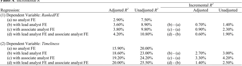
Table 2 reports the results from estimating Eq. (1) to test the relative contribution of lead analysts and associate analysts to the variation in forecast accuracy and timeliness. Panel A lists the changes in R2 with and without lead or associate analyst fixed effects. Panel B presents the coefficient estimates for the control variables. Panel C provides the F-statistics and p-values for the lead analyst and associate analyst fixed effects. Lastly, Panel D shows the partial effect of the lead and associate analyst fixed effects on total R2.
Panel A suggests that associate analyst fixed effects improve the explanatory power of the model for forecast accuracy. The adjusted R2 of the baseline model is 2.90 percent. Associate analyst fixed effects increase the adjusted R2 by 0.90 percent, compared to an increase of 0.70 percent when including lead analyst fixed effects. Including associate analyst fixed effects in addition to lead analyst fixed effects increases the adjusted R2 by 0.60 percent, representing an improvement of 16.67 percent (= 0.60 / 3.60) in the model’s explanatory power. We also examine the statistical significance of associate analyst fixed effects. F-test statistics in Panel C indicate that associate analyst fixed effects are significantly different from zero at the aggregate (F-statistic = 1.393, p-value < 0.001). In summary, the results provide initial support that associate analysts explain a significant amount of the variation in forecast accuracy.
Panel D presents the partial contribution of the lead and associate analyst fixed effects to the total R2. Following Graham et al. (2010), we decompose and allocate total R2to lead and associate analyst fixed effects. The decomposition shows that lead analyst fixed effects explain 1.40 percent of the variation in forecast accuracy (12.96 percent of the total R2); while associate
20
analyst fixed effects explain 2.10 percent of the variation in forecast accuracy (19.44 percent of the total R2). The last row in Panel D compares the explanatory power of lead analyst fixed effects to the explanatory power of associate analyst fixed effects. The value of 0.667 implies that associate analyst fixed effects explain 49.90 percent more of the variation in forecast accuracy than lead analyst fixed effects do (= 1 / 0.667 – 1). This finding is consistent with our prediction that lead analysts delegate the forecasting of earnings to their associate analysts.16
The relative contribution of lead analysts and associate analysts to the variation in forecast timeliness
Regression results of the relative importance of lead analysts and associate analysts to forecast timeliness are reported in column 2 of Table 2. A higher value of Timeliness represents more timely estimates. Panel A shows that the adjusted R2 increases by 3.30 percent when we add associate analyst fixed effects to the baseline model. Adding associate analyst fixed effects to the model with lead analyst fixed effects increases the adjusted R2 by 1.40 percent. F-test statistics in Panel D show that both lead and associate analyst fixed effects are statistically different from zero, with p-values below 0.001. These results suggest that associate analysts contribute to the variation in forecast timeliness.
Panel D presents the total R2 allocation to the lead and associate analyst fixed effects. We find that lead analyst fixed effects explain 6.20 percent of the variation in timeliness (24.31
16 Note that our sample is different from prior studies (e.g., Clement 1999 and Jacob et al. 1999) in that we examine a subset of four brokerage houses and a different sampling period. The coefficient estimate on Freq is significantly positive while Jacob et al. (1999) observe a negative or statistically insignificant coefficient. Our finding is driven by the use of all analyst-firm-quarter observations while Jacob et al. (1999) restrict their sample to the last forecast of a given analyst for a specific firm-quarter. We deviate from Jacob et al.’s (1999) sample restriction to allow for the same sample size across all analyses. It is important for us to maintain a constant sample size across analyses since R2 is significantly impacted by sample size. Notwithstanding, in untabulated analyses we restrict the sample to the last forecast for a given analyst-firm-quarter. All inferences are qualitatively unchanged, and the coefficient estimate on Freq is negative, consistent with the findings of Jacob et al. (1999).
21
percent of total R2)while associate analyst fixed effects explain 3.60 percent of the variation in timeliness (14.12 percent of total R2). The results in the last row show that lead analyst fixed effects explain 1.722 times as much of the variation in forecast timeliness as associate analyst fixed effects do. These results suggest that the decision to issue a forecast is at the discretion of the lead analyst. Furthermore, these findings suggest that the higher explanatory power of associate analyst fixed effects when the dependent variable is forecast accuracy is not attributed to the larger number of associate analyst fixed effects; otherwise we would have observed comparable results for forecast timeliness.
The coefficient estimates are presented in Panel B. The coefficient estimate on forecast horizon (Horizon) is 0.042 (t-statistic = 7.38), implying that forecasts issued earlier in the quarter are more likely to be timelier. Moreover, the results suggest that forecast timeliness also improves with the lead analyst’s firm-specific experience (LnFirmExperience), with a coefficient estimate of 0.823 (t-statistic = 5.25). The frequency of analyst reports (Freq) is negatively associated with timeliness. This result is expected since most analysts in our sample issue one forecast per firm-quarter. Therefore, given the definition of forecast timeliness, a follow-up forecast is compared to the forecasts at the beginning of the quarter, resulting in a lower timeliness value. Lastly, the coefficient estimate on the percentage of analysts joining the brokerage house (PIN) is negative and significant. This findings can be explained by either the new analysts that joined the brokerage house are not able to issue forecasts in proximity to the prior earnings announcements, or by changes to the resource allocation at the brokerage house that affect all analysts at the brokerage house.
22
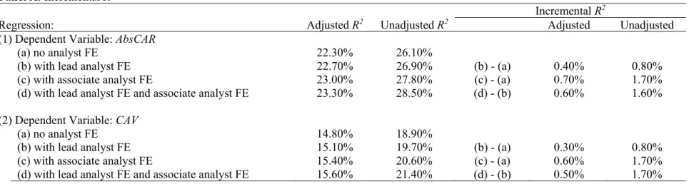
The relative contribution of lead analysts and associate analysts to the variation in stock price reaction and abnormal trading volume
We present the results for the relative contribution of lead analyst and associate analyst fixed effects to the variation in stock price reaction and abnormal trading volume in Table 3. Panel A comparesthe model R2s with and without lead or associate analyst fixed effects. For stock price reaction (abnormal trading volume), adding associate analyst fixed effects to the baseline regression increases the adjusted R2 by 0.70 (0.60) percent. Including associate analyst fixed effects in addition to lead analyst fixed effects increases the adjusted R2 by 0.60 (0.50) percent. Panel C presents the results for the F-tests that examine the statistical significance of the lead and associate analyst fixed effects. The p-values for both the lead analyst fixed effects and associate analyst fixed effects are below 0.001 in both columns, implying that both lead analyst fixed effects and associate analyst fixed effects explain a significant portion of the variation in the stock price reaction and abnormal trading volume.
Panel D shows that for stock price reaction (abnormal trading volume), the total R2 attributed to lead analyst fixed effects is 0.028 (0.032), while the total R2 attributed to associate analyst fixed effects is 0.015 (0.011). The bottom row shows that lead analyst fixed effects explain 86.70 (190.90) percent more of the variation in stock price reaction (abnormal trading volume) than associate analyst fixed effects do. In summary, the results in Table 3 suggest that lead analysts dominate associate analysts in their contribution to the variation in stock price reaction and abnormal trading volume. These results are consistent with our prediction that lead analysts are more involved in the qualitative component of analyst reports, as captured by the stock market variables. However, our results may also be attributed to the lead analyst’s reputation and visibility, which induce more trading volume and a higher price reaction.
23
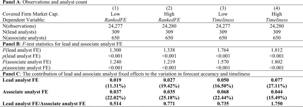
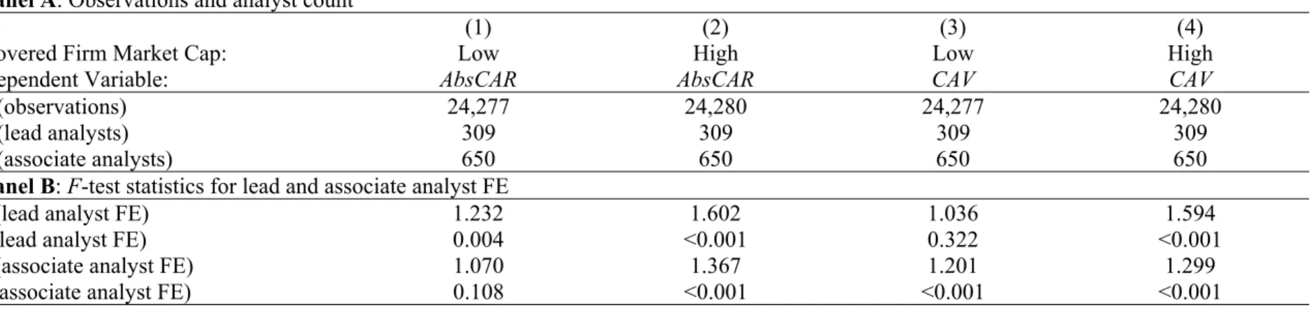
The moderating effect of firm size on the explanatory power of lead and associate analyst fixed effects
Tables 4A and 4B present the results for testing Hypothesis 3 on the moderating effect of firm size on the relative impact of lead and associate analysts on analyst reports. We present the number of observations and the number of lead and associate analysts included in each subsample in Panel A. Results for the F-tests for lead and associate analyst fixed effects are provided in Panel B and the results of the partial effect of lead and associate analyst fixed effects on total R2 are presented in Panel C.
We partition the sample by the median market cap at the previous quarter-end date by lead-associate analyst pair. We use this cutoff instead of the sample median for two reasons. First, analysts may cover only large cap or small cap firms because of industry characteristics or analysts’ expertise. Partitioning by lead-associate analyst pairs ensures comparison of firm sizes within an analyst’s portfolio rather than across different analyst portfolios. Second, subsampling by lead-associate analyst pairs ensures that the same groups of lead and associate analysts are included in both subsamples. Consequently, all the columns in tables 4A and 4B include 309 unique lead analysts and 650 unique associate analysts.
Columns 1 and 2 in Panel C of Table 4A show that, for forecast accuracy, the explanatory power of lead analyst fixed effects is 11.31 percent (19.42 percent) of total R2 for firms with a market cap below (above) the median, respectively. The relative contribution of lead analyst fixed effects (compared to that of associate analyst fixed effects) for forecast accuracy is 50.00 percent larger (= 0.771 / 0.514 – 1) for larger firms. Similarly, for forecast timeliness, columns 3 and 4 show that the explanatory power of lead analyst fixed effects is 16.50 percent (27.11 percent) of total R2 for firms with a market cap below (above) the median, respectively. The relative contribution of lead analyst fixed effects (compared to associate analyst fixed effects) for forecast
24
timeliness is 138.10 percent larger (= 1.750 / 0.735 – 1) for larger firms. Panel C of Table 4B shows that the explanatory power of lead analyst fixed effects for both stock price reaction and abnormal trading volume is higher when the covered firm’s size is larger. Overall, the results in Table 4 suggest that lead analysts are more involved in the coverage of firms that are more significant to revenue generation at the brokerage house.
The moderating effect of lead analysts’ firm-specific experience on the explanatory power of lead and associate analyst fixed effects
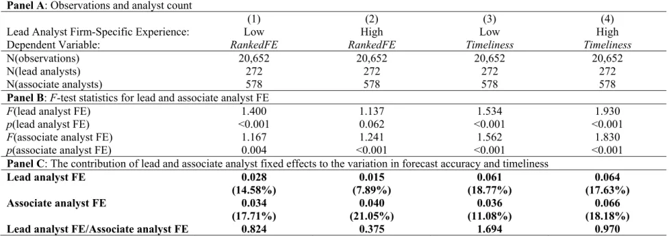
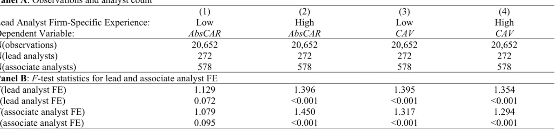
Tables 5A and 5B report the results for testing Hypothesis 4 on the effect of lead analysts’ firm-specific experience on the relative contribution of lead and associate analyst fixed effects. We partition the sample at the median value of the lead analyst’s firm-specific experience by lead-associate analyst pair. Like the partition on firm size, we subsample by lead-lead-associate analyst pair to ensure the same groups of lead and associate analysts appear in both subsamples. Consequently, all the analyses include 272 unique lead analysts and 578 unique associate analysts.
Columns 1 and 2 in Panel C of Table 5A compare the changes in the partial effects of lead and associate analyst fixed effects on the total R2. When lead analysts’ firm-specific experience is low, lead analyst fixed effects explain 17.65 percent less of the variation in forecast accuracy than associate analyst fixed effects do (= 0.028 / 0.034 – 1). However, when lead analysts’ experience is above the median, lead analyst fixed effects explain 62.50 percent less of the variation in forecast accuracy relative to associate analyst fixed effects (= 0.015 / 0.040 – 1). The results in columns 3 and 4 for timeliness and in Table 5B for stock price reaction and abnormal trading volume are qualitatively similar. These results suggest that as lead analysts cover a firm for a longer period of time, they delegate more tasks to their associates. These results suggest that lead analysts are more involved during the initiation a coverage, when significant learning and
25
information processing is required. Over time, as the model improves, lead analysts delegate more tasks to the associate analysts.
The moderating effect of associate analysts’ firm-specific experience on the explanatory power of lead and associate analyst fixed effects
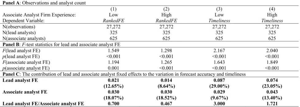
Tables 6A and 6B present the results for testing Hypothesis 5 on the effect of associate analysts’ firm-specific experience on the relative contribution of lead and associate analyst fixed effects. Since associate analysts’ firm-specific experience is only observed for analyst reports authored with associate analysts, we first partition the sample by the median value of the associate analyst’s firm-specific experience by lead-associate analyst pair. We then include sole-authored reports in both partitions of the sample, when available, to ensure robust identification of lead and associate analyst fixed effects. All subsamples in Table 6A and 6B contain 325 unique lead analysts and 625 unique associate analysts.
Columns 1 and 2 in Panel C of Table 6A show a decrease in the partial effects of lead relative to associate analyst fixed effects on the total R2 when associate analysts are more experienced. When associate analysts’ firm-specifc experience is low, lead analyst fixed effects explain 30.00 percent less of the variation in forecast accuracy than associate analyst fixed effects do (= 0.021 / 0.030 – 1). When associate analysts’ firm-specific experience is above the median, lead analyst fixed effects explain 53.33 percent less of the variation in forecast accuracy relative to associate analyst fixed effects (= 0.014 / 0.030 – 1). Columns 3 and 4 indicate that when associate analysts’ firm-specific experience is low, lead analyst fixed effects explain 3 times as much of the variation in forecast timeliness as explained by associate analyst fixed effects. When associate analysts’ experience is above the median, lead analyst fixed effects explain 72.10 percent more of the variation in forecast timeliness than associate analyst fixed effects do. These
26
results are consistent with our conjecture that lead analysts are more involved in forecasting in the early stages of training of associate analysts. We obtain qualitatively similar inferences when we examine stock price reaction and abnormal trading volume in Table 6B.
The moderating effect of forecast timing on the explanatory power of lead and associate analyst fixed effects
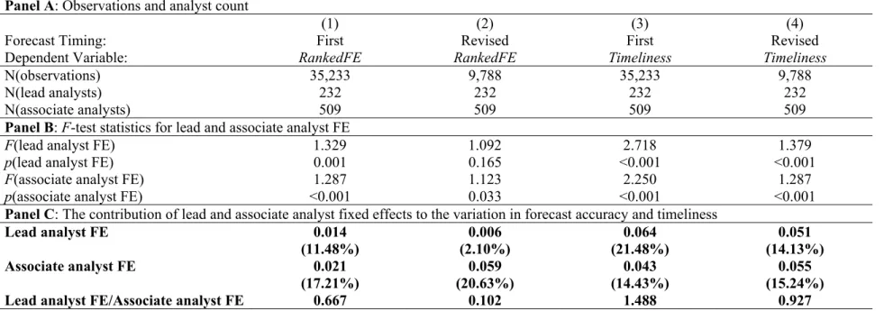
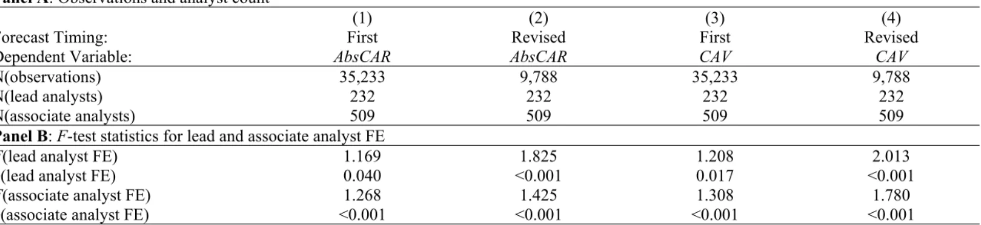
Tables 7A and 7B provide the results for testing Hypothesis 6 on the effect of forecast timing on the relative explanatory power of lead and associate analyst fixed effects. The sample is partitioned by the first and revised forecasts, where the first forecast is defined as the first forecast following the earnings announcement for the previous quarter and the revised forecast is defined as any forecast revision made after the first forecast and before the earnings announcement for the current quarter. Lead-associate pairs who have never issued a revised forecast during our sampling period are removed to ensure the same groups of lead and associate analysts are included in all subsamples. Thus, all subsamples cover 232 unique lead analysts and 509 unique associate analysts.
The results in columns 1 and 2 in Panel C of Table 7A show that the relative contribution of lead analyst fixed effects (compared to associate analyst fixed effects) for forecast accuracy decreases from 0.667 for the first forecast in the quarter to 0.102 for the revised forecast in the quarter. The decline in relative contribution is attributed to a simultaneous decrease in the explanatory power of lead analyst fixed effects (from 11.48 percent of total R2 to 2.10 percent of total R2) and an increase in the explanatory power of associate analyst fixed effects (from 17.21 percent of total R2 to 20.63 percent of total R2). Consistent with the decrease in the explanatory power of lead analyst fixed effects, the F-statistics in Panel B indicate that lead analyst fixed effects are significant for the first forecasts but insignificant for the revised forecasts. These
27
results suggest that lead analysts are more involved in modeling the first forecast in the quarter, when more information processing is required. The results are also consistent with lead analysts’ increased involvement in tasks that generate more trading commissions since the first forecast in the quarter is more informative than the revised forecast (Amiram et al. 2016). Similar to the results for forecast accuracy, we find in columns 3 and 4 of Table 7A Panel C that the explanatory power of lead analyst fixed effects (compared to that of associate analyst fixed effects) for forecast timeliness decreases from 1.488 for the first forecasts to 0.927 for the revised forecasts. The results indicate that lead analysts delegate the choice of whether and when to issue the revised forecast to the associate analyst, possibly due to the lower importance of the revised forecast compared to the first forecast in the quarter.
Table 7B, Panel C shows that the explanatory power of lead analyst fixed effects relative to that of associate analyst fixed effects increases in the revised forecasts. While this result is counter-intuitive, a possible explanation for the increase is that lead analysts are busier during the earnings announcements season, and they therefore have more time to invest in the qualitative aspect of the revised reports.
6. Additional discussion
Assortative matching
A clean identification of lead and associate analysts requires random assignment, i.e., associate analysts are randomly assigned to lead analysts. However, such assumptions are not attainable in practice as lead analysts usually participate in the interview process of associate analysts and have a certain level of freedom to pick associate analysts with whom they want to work. In this section, we explain why we do not expect such potential assortative matching between lead and associate analysts to affect the interpretation of our results.
28
First, assortative matching between lead and associate analysts may be based on analyst competence, e.g., the best-performing lead analysts may have the first pick of the most promising associate analysts. To address this kind of assortative matching, in untabulated analyses, we include additional controls for associate analysts’ firm experience, the industry specialization of associate analysts, and the number of firms covered by associate analysts to capture associate analysts’ competence and expertise (the construction of those variables is comparable to the construction of lead analyst controls). The inclusion of those associate analyst variables does not change the inferences from the results.
Second, assortative matching between lead and associate analysts can also be based on other unobservable traits. For example, lead analysts with specialized industry background (e.g. an M.D. degree) may prefer associate analysts with accounting and finance expertise. If a lead analyst consistently picks a certain type of associate analysts, the lead analyst fixed effects will partially absorb the effects of the common associate analyst traits. In other words, the impact of lead analyst fixed effects on analyst reports will be over-estimated and the impact of associate analyst fixed effects will be under-estimated. Jointly, the results will be biased towards lead analysts. If this bias is large, we will observe a consistently larger partial effects of lead analyst fixed effects compared to associate analyst fixed effects on the total R2 for all dependent variables, which is not the case for forecast accuracy. Thus, we do not expect this bias to be significant to qualitatively alter our inferences from the main results. As for the cross-sectional tests, since we include the same groups of lead and associate analysts in the partitioned samples, the assertive matching impact, to the extent that it exists, should be similar for both subsamples that we compare. Thus, a comparison between the two subsamples eliminates the assortative matching effect.
29
Overall, assortative matching can affect the values of each individual partial effects of lead and associate analyst fixed effects on the total R2, but we do not expect this issue to materially alter the interpretation of our results.
The validity of fixed-effect estimation
Fee, Hadlock, and Pierce (2013) discuss the limitations of using fixed effects to identify the impact of CEOs’ idiosyncratic-style on firms’ investment and financing decisions, and document that CEO fixed effects are falsely significant in a simulated sample. In this section, we compare the setting of our paper to the CEO setting and discuss why the limitations that impair the validity of fixed effects in their study do not apply in our setting.
Fee et al. (2013) discuss two major limitations of using CEO fixed effects to identify CEO’s idiosyncratic-style on the firm’s investment and financing decisions. First, the identification of CEO fixed effects relies on individuals who have served as CEOs in different firms. However, CEOs rarely move, and, even if they do move, they usually only move once. Further, the rarity of CEO relocation raises concerns that CEO job movers are not representative of the CEO population (i.e., only certain types of CEOs move) or that the results are driven by confounding factors other than CEOs’ idiosyncratic-style (i.e., CEOs only move under certain circumstances). In contrast, our setting has considerably more variation in the coverage of firms and authorship of the reports. In our sample, lead analysts and associate analysts cover, on average, 19.157 and 14.314 firms, respectively. Further, 85.26 percent of analyst reports are issued by lead analysts who have at least sole-authored once during the sample period, and 86.12 percent of analyst reports are issued by lead analysts who have worked with more than one associate analyst. The adequate variation in firm coverage and report authorship allows a more
30
precise identification of firm, lead, and associate analyst fixed effects, and thus our results are more representative of the analyst population and less sensitive to potential confounding factors. Second, a firm’s investment and financing policies are expected to be highly positively serially correlated. Such serial correlation, along with the use of long time-series data and fixed effects, can lead to the underestimation of standard errors (Bertrand, Duflo, and Mullainathan 2004; Fee et al. 2013). In Fee at al.’s (2013) simulated sample, the three factors reinforce each other to facilitate a spurious significance of CEO fixed effects, which capture the difference in the serial correlation structure of the two firms’ policies rather than the influence of CEOs’ idiosyncratic-style. This issue is not material in our setting for two reasons. First, we do not rely on the F-tests to examine the significance of lead and associate analyst fixed effects. Instead, we focus on the partial effect of lead and associate analyst fixed effects on the total R2, which is not impacted by this issue. Second, our sample includes analysts that issue sole-authored reports (which is not possible in the CEO setting since it is uncommon for firms to be without a CEO) and has significantly more variation because lead and associate analysts cover multiple firms. Therefore, the effect of the serial correlation of our dependent variables on the standard errors in our setting is likely to be smaller compared to the CEO setting. Overall, we do not expect the limitations of the CEO setting to apply to the analyst setting.
7. Conclusion
Extant research examines the determinants of analysts’ performance. In those studies, the presumption, supported by “star” analyst rankings, is that sell-side equity research is individual. However, analysts usually work in hierarchical teams that are led by a senior analyst, who is also the “face” of the team. Using a hand-collected sample of analyst teams from four brokerage
31
houses that we obtain from analyst reports, we examine the role of associate analysts in explaining lead analysts’ performance. We posit that the division of labor between lead and associate analysts follows a “pecking order” where lead analysts focus on higher importance tasks and delegate other tasks to associate analysts.
We find that associate analyst fixed effects explain more of the variation in lead analysts’ forecast accuracy than lead analyst fixed effects do. In contrast to our findings for forecast accuracy, we document that lead analysts explain more of the variation in forecast timeliness and the stock price reaction to analyst reports. These results suggest that EPS forecasting is delegated to associate analysts. However, the decision to issue a report, captured by timeliness, and the qualitative component of the report, as captures by the stock price reaction and abnormal trading volume, are the main responsibility of the lead analyst. These findings are consistent with surveys of institutional investors, which suggest that communication skills and industry knowledge are more important analyst traits than the quality of earnings estimates.
In cross-sectional tests, we find that lead analysts are more involved in the coverage of large firms. Sell-side equity research generates revenues from trading commissions and larger firms typically generate more trading volume. This finding suggests that lead analysts are more involved in covering firms that generate more revenues to the brokerage house. We also document that lead analysts’ involvement decreases with their firm-specific experience. These results suggest that lead analysts are more involved when more expertise and information processing are required. Next, we find that lead analysts’ involvement in composing analyst reports and earnings estimates decreases with the associate analyst’s firm-specific experience, which suggests that lead analysts assign more tasks to associates as the associates become more experienced. Lastly, we document that lead analysts are more involved in creating the first forecast in the quarter
32
compared to revised forecasts. These results are consistent with lead analysts’ increased involvment in higer importance tasks and when more information processing is required.
Our study extends the literature by documenting that, despite lead analysts having been the focus of extant academic research, associate analysts also play a significant role in forecasting. Our findings inform on a major debate in the analyst literature. Despite the extensive research on the determinants of forecast accuracy, it is still unclear whether forecast accuracy is important to analysts. On the one hand, multiple studies find that low forecast accuracy is associated with turnover. On the other hand, additional studies find that forecast accuracy is not associated with analyst compensation and “star” status, and surveys of buy-side analysts suggest that forecast accuracy is not a primary objective for sell-side analysts. Our study contributes to this debate by documenting that lead analysts delegate forecasting to associate analysts. Therefore, while forecast accuracy may not be a first-order task for lead analysts, our findings suggest that it may be a first-order task for associate analysts.
33 References
Amiram, D., E. Owens, and O. Rozenbaum. 2016. Do information releases increase or decrease information asymmetry? New evidence from analyst forecast announcements. Journal of Accounting and Economics 62(1): 121–138.
Bagnoli, M., M. Beneish, and S. Watts. 1999. Whisper forecasts of quarterly earnings per share.
Journal of Accounting and Economics 28(1): 27–50.
Bertrand, M., E. Duflo, and S. Mullainathan. 2004. How much should we trust difference-in-difference estimates? Quarterly Journal of Economics 119(1): 249–275.
Bertrand, M., and A. Schoar. 2003. Managing with style: The effect of managers on firm policies. The Quarterly Journal of Economics 118 (4): 1169–1208.
Beyer, A., D. Cohen, T. Lys, and B. Walther. 2010. The financial reporting environment: Review of the recent literature. Journal of Accounting and Economics 50(2-3): 296–343. Bradshaw, M. T. 2004. How do analysts use their earnings forecasts in generating stock recommendations? The Accounting Review 79(1): 25–50.
Bradshaw, M. T. 2011. Analysts’ forecasts: what do we know after decades of work? Unpublished working paper.
Bradshaw, M. T., M. S. Drake, J. N. Myers, and L. A. Myers. 2012. A re-examination of
analysts’ superiority over time-series forecasts of annual earnings. Review of Ac