Acceleration Methods for Ray Tracing based
Global Illumination
Dissertation
zur Erlangung des Doktorgrades Dr. rer. nat.
der Fakultät für Ingenieurwissenschaften und Informatik der Universität Ulm
vorgelegt von
Holger Dammertz
aus München
Ulm University, Germany Gutachter: Dr. rer. nat. Alexander Keller,
mental images, Berlin
Gutachter: Prof. Dr.-Ing. Hendrik P. A. Lensch, Ulm University, Germany
Externer Gutachter: Peter Shirley, Adjunct Professor, Ph.D. University of Utah, Salt Lake City, UT, USA Tag der Promotion: 19.04.2011
The generation of photorealistic images is one of the major topics in computer gra-phics. By using the principles of physical light propagation, images that are indistin-guishable from real photographs can be generated. This computation, however, is a very time-consuming task. When simulating the real behavior of light, individual images can take hours to be of sufficient quality. For this reason movie production has relied on artist driven methods to generate life-like images. Only recently there has been a convergence of techniques from physically based simulation and movie production that allowed the use of these techniques in a production environment. In this thesis we advo-cate this convergence and develop novel algorithms to solve the problems of computing high quality photo-realistic images for complex scenes. We investigate and extend the algorithms that are used to generate such images on a computer and we contribute novel techniques that allow to perform the necessary ray-tracing based computations faster. We consider the whole image generation pipeline starting with the low level fundamentals of fast ray tracing on modern computer architectures up to algorithmic improvements on the highest level of full photo-realistic image generation systems.
In particular, we develop a novel multi-branching acceleration structure for high per-formance ray tracing and extend the underlying data structures by software caching to further accelerate the result. We also provide a detailed analysis on the factors that influence ray tracing speed and derive strategies for significant improvements. These create the foundations for the development of a production quality global illumination rendering system. We present the system and develop several techniques that make it usable for realistic applications. The key aspect in this system is a path space par-titioning method to allow for efficient handling of highly complex illumination situations as well as the handling of complex material properties. We further develop methods to improve the illumination computation from environment maps and provide a filtering technique for preview applications.
Many thanks to
• Alexander Keller for his guidance, support, and his passion for computer graphics • Johannes Hanika for a fun and highly productive research cooperation
• Hendrik P. A. Lensch for his feedback, support and for providing the environment to finish this Ph.D. thesis
• the old and new computer graphics group • mental images for the financial support
• Carsten Wächter, Matthias Raab, Leonhard Grünschloss, and Daniel Seibert for proofreading and many rendering related discussions
1 Introduction 1
1.1 Physically Based Rendering and Visual Effects . . . 2
1.2 Thesis Overview . . . 2
1.2.1 Summary of Contributions . . . 3
2 Image Generation Fundamentals 5 2.1 Image Generation by Camera Simulation . . . 5
2.2 Light Transport Simulation by Path Tracing . . . 8
2.3 Rendering Software Architecture Design . . . 9
2.3.1 Enabling Physically Based Global Illumination in Movie Production 9 2.3.2 Scene Description . . . 10
2.3.3 Boundary Representation . . . 11
2.3.4 Material Representation . . . 15
2.3.5 Sampling Light Sources . . . 18
2.4 Processor Architecture . . . 20
3 Efficient Tracing of Incoherent Rays 31 3.1 Overview of Acceleration Data Structures . . . 33
3.1.1 Bounding Volume Hierarchies . . . 33
3.1.2 kd-Trees . . . 34
3.1.3 Grids . . . 35
3.2 n-ary Bounding Volume Hierarchies . . . 36
3.3 Investigation ofn-ary Hierarchy Traversal . . . 38
3.3.1 Data Structures for Traversal . . . 38
3.3.2 Unsorted Traversal . . . 41
3.3.3 Sorted Traversal . . . 42
3.3.4 t-Far Stack for Early Out . . . 48
3.5.1 Rendering Performance . . . 50
3.5.2 Memory Bound Performance . . . 51
3.5.3 Explicit Coherence in Ray Tracing . . . 51
4 Efficiency of Hierarchies 57 4.1 Overview of Hierarchy Construction Heuristics . . . 58
4.1.1 Median Split . . . 59
4.1.2 Center Split . . . 59
4.1.3 Surface Area Heuristic (SAH) . . . 60
4.2 Split Heuristics for the QBVH . . . 61
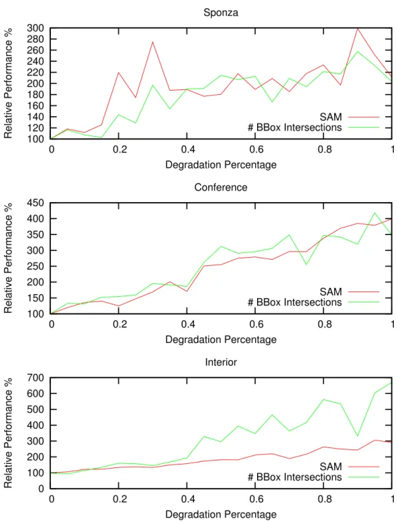
4.2.1 Visual Comparison of Center-Split and SAH-Split . . . 62
4.2.2 Validity of the SAH for Physically Based Rendering . . . 62
4.3 More Efficient Hierarchies by Triangle Subdivision . . . 66
4.3.1 Edge Volume Heuristic . . . 67
4.3.2 Bounding Box Area Heuristic (BBAH) . . . 72
4.3.3 Leaf Compaction . . . 74
4.3.4 Triangle Subdivision and the SAH . . . 75
4.4 Crack-Free Triangle Intersection . . . 82
4.5 SAH Clustering for Ray Tracing of Dynamic Scenes . . . 83
4.6 Discussion . . . 90
5 Software Caching for Ray Tracing 91 5.1 Triangle Intersection and SIMD Caching . . . 92
5.2 Parallel Triangle Intersection . . . 97
5.3 Accelerating Shadow Rays . . . 98
5.4 Discussion . . . 104
6 Practical Physically-Based Image Synthesis 105 6.1 Principles of Light Transport Simulation . . . 106
6.1.1 Path Tracing . . . 107
6.1.2 Light Tracing . . . 108
6.1.3 Photon Mapping . . . 108
6.1.4 Instant Radiosity . . . 112
6.2 Hierarchical Monte Carlo Integro-Approximation . . . 112
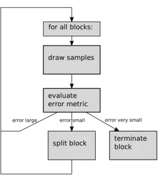
6.2.1 Monte Carlo Integration and Monte Carlo Integro-Approximation . 113 6.2.2 Iterative Block Partitioning and Termination . . . 114
6.2.3 Adaptive Light Tracing . . . 118
6.2.4 Results and Discussion . . . 119
6.3 Path Space Partitioning . . . 125
6.3.1 Eye Path Generation and Glossy Effects . . . 130
6.3.2 Point-Light-Based Diffuse Illumination . . . 132
6.3.3 Caustic Histogram Method . . . 133
6.3.6 Discussion . . . 141
6.4 High Dynamic Range Environment Map Lighting . . . 146
6.4.1 Domains of Integration . . . 146
6.4.2 Plane Sampling for Starting Light Paths from Environment Maps . 148 6.4.3 Results and Discussion . . . 150
6.5 Interactive Preview for Design and Editing . . . 153
6.5.1 Edge-Avoiding À-Trous Irradiance Filtering . . . 155
6.5.2 Implementation . . . 159
6.5.3 Results . . . 162
6.5.4 Discussion . . . 167
6.6 On Demand Spectral Rendering . . . 169
6.6.1 Lens Simulation . . . 170
6.6.2 Fluorescent Concentrator Simulation . . . 175
7 Conclusion 179 7.1 Future Work . . . 180 List of Tables 181 List of Figures 183 Listings 187 Bibliography 189
1
Introduction
One of the strongest driving forces in computer graphics has been the strive to repro-duce reality. Starting with the beginning of graphical computer displays, scientists and artists alike pushed the boundaries of what is possible. Over the years, computer gen-erated images were able to approximate the appearance and phenomena of the real world better and better. While in the beginning only primitive shapes, a limited color space, and simple algorithms could be used to approximate reality, the huge advance-ments in computing power over the last 20 years as well as significant improveadvance-ments in the fundamental algorithms allow us to now generate images and movies entirely in the computer. The results are almost impossible to distinguish from real photographs or live footage.
Even though high quality computer generated images are now a reality there is a large area of unsolved problems and a lot of room for improvement. The simulation of the phenomena from nature is a highly complex and compute-intensive task. Especially for the production of movies, where thousands of individual images are needed, speed as well as quality is of paramount importance. The goal of increased realism is tightly coupled with increasing complexity. While in the beginning of computer graphics the realistic rendering of a single object was an enormous task, nowadays whole cities and forests are modeled in a computer and rendered into realistic images.
1.1 Physically Based Rendering and Visual Effects
Physically based rendering is a sub-class of graphics algorithms that use real physical quantities and models to not only produce visually pleasing but also quantitatively cor-rect images. The corcor-rectness of the image is of course only valid within the constraints of the physical model that is used but nevertheless allows to produce results that can be measured in the real world. This approach is in stark contrast to artist driven methods that are used for real time computer graphics as well as for movie production. While the visual effects in movies look strikingly realistic since over a decade now, their rendering methods do not rely on realistic physical simulations but on handcrafted models and artist tweaked parameters to achieve the desired results. Only recently this has begun to change and the visual effects industry as well as the real time graphics community have realized the advantage realistic models can provide over manual crafting. Even though one can always argue that artistic freedom is important for visual effects and real time graphics, the advantages of being able to simulate light and surfaces as they behave in the real world cannot be neglected. In this thesis we advocate this conver-gence and present novel algorithms that improve the robustness as well as the speed of physical light transport simulation.
1.2 Thesis Overview
One very general way to simulate the distribution of light is by tracing individual light rays through the scene and modeling their behavior like reflection or refraction using physical models. This basic operation is realized by an algorithm called ray tracing and is one of the fundamental building blocks that we use in this thesis. Based on this foundation, we will develop novel acceleration methods for fast incoherent ray tracing and several new techniques and improvements for physically based rendering algorithms. Our ray tracing algorithm acceleration methods directly benefit all simulation algorithms devel-oped in this thesis and we show their effectiveness in a complete rendering system that uses all our results. Some of the algorithms and results presented in this thesis have already been published at conferences and in different journals [Damm 06, Damm 08a, Damm 08b, Bend 08, Damm 09a, Damm 09b, Damm 10a, Damm 10b]. We present this research in a unified framework and give additional results and discussions. We will also extend the work at several points and present new techniques and insights.
The remainder of this thesis is organized as follows. In Chapter 2 we will review the fundamentals of image generation and discuss the basic framework of a rendering system. We also discuss some fundamentals of processor architectures that are re-quired for high performance rendering applications. Chapter 3 develops our novel data structure for accelerated ray tracing specifically optimized for physically based render-ing problems and Chapter 4 further improves this data structure by considerrender-ing the representation of the 3d scenes and the hierarchy construction algorithm. In Chapter 5 we will consider software caching for improving the ray tracing performance in light transport simulations.
Chapter 6 then introduces a full-featured, general global illumination system for pro-duction quality image generation. This system is built on top of the data structures and acceleration techniques developed in the previous chapters and addresses many of the problems encountered in image generation for visual effects with physically based rendering systems. In this chapter we will contribute several techniques for global illumi-nation computation like an environment map sampling technique and an image-space filter for interactive preview. Finally, in Chapter 7 we will summarize the developed techniques and discuss their relationships.
1.2.1 Summary of Contributions
To summarize, the main contributions in this thesis are
• a novel bounding volume hierarchy for acceleration of incoherent rays. This ac-celeration structure is targeted towards modern hardware architectures, performs significantly faster than previously used structures, and requires less memory than previous methods.
• an efficient triangle splitting heuristic that improves the quality of ray tracing ac-celeration structures in many situations.
• an iterative ray-triangle intersection algorithm that guarantees that no intersec-tions are missed. This is often needed in physical simulaintersec-tions where accuracy is paramount.
• a discussion of software caching for ray tracing acceleration with a branch-free parallel triangle intersection algorithm and a novel shadow cache that can greatly improve the efficiency of visibility queries.
• a global iterative stopping criterion for Monte Carlo light transport simulation based on integro-approximation.
• a path space partitioning method that, contrary to previous algorithms, solves the full light transport equation by several distinct algorithms. With this method we develop a production quality global illumination renderer that has less restrictions than previous methods (for example allowing for non-physical BRDFs).
• an environment map sampling technique that allows to start light paths with cor-rect Monte Carlo weights.
• an image-space filtering technique for noisy Monte Carlo images that allows for fully interactive real-time preview of illumination and material changes.
• a discussion of on-demand spectral rendering with application examples in fluo-rescent concentrator simulation and a spectral camera lens simulation.
2
Image Generation Fundamentals
In this Chapter we will provide the fundamentals of the image generation pipeline and basic architecture considerations that are needed to understand the rest of this thesis.
2.1 Image Generation by Camera Simulation
It is our goal to create an efficient computer program to generate synthetic images that are indistinguishable from real images. One point of view to explain this process is by considering how real images are acquired into a computer processable format by a camera. The computer program now tries to replicate this process as closely as possible to generate a final image.
Raster Images
A computer generated image is stored as an array of color values. Each color value represents usually a square in the image region called a pixel (short for picture ele-ment) but the square layout is not necessary [Damm 09c]. Most computer generated images are displayed on computer monitors that have three color components per pixel called RGB. They correspond to the red, green and blue channel, each of which has a
resolution of an8 bit integer (values between 0and 255). There exist other standards
and, especially for print, other representations but in this thesis we will use the8bit per
channel RGB representation with square pixels as final output. Figure 2.1 illustrates the data layout and representation.
Figure 2.1: Illustration of a pixel raster and an image stored in the raster. The left figure shows a pixel raster of the size 10×7. The right figure shows the same
image on a pixel raster with the resolution 320×224pixels. As an overlay
the raster of the left image is shown.
Dynamic Range vs. Tone Mapping
In nature, brightness differences have a very high dynamic range. Most commonly used display technologies cannot reproduce this. They provide usually only8 bits per
chan-nel for the final output. Nevertheless, internal representations during image synthesis need a higher resolution and range. Throughout this thesis we will use the RGB for-mat, but with32bit floating point numbers per channel if not otherwise noted. A short
overview of floating point numbers can be found in Section 2.4. This allows to perform all computations directly inside the image buffer without losing too much accuracy. This is necessary for high quality photo-realistic image synthesis. The representation using floating point numbers is sometimes called high dynamic range representation (HDR) as it allows for huge value differences using the exponent of the float representation. Even though there exist approaches to directly display images with a higher dynamic range [Seet 04], for most display devices the dynamic range of the image has to be mapped to a smaller displayable range. This is performed with tone mapping opera-tions. In Chapter 22 of [Shir 02] an overview of tone reproduction for computer graphics can be found. A commonly used tone-mapping operator is described by Reinhard in [Rein 02]. A comparison of five recent operators can be found in [Ashi 06].
The simplest operator to use is by normalizing the luminance of the color value: Lnew =
L L+ 1
The luminance is computed by transforming the RGB value into a color-space with a luminance channel like HSV.
For combining computer generated images with real world images in movie produc-tion a high dynamic range in the stored output image is also very important. To achieve realistic results the response curve of the film has to be modeled and used to adjust the computer generated image. The closer the simulation is to real world parameters the easier it becomes to adjust the computer generated images.
Ray Tracing
Ray tracing is a fundamental technique to create computer generated images. It was first developed in 1968 by Appel in [Appe 68] as a method to add shadows to a computer generated image. Since then a lot of research started on using ray tracing for computer graphics and image generation.
In its basic form ray tracing computes computer generated images by computing a color value for each pixel independently of all the other pixels. To generate an image several components are needed. First is a camera that defines the viewer (or eye) posi-tion in the scene and also the viewing direcposi-tion. Coupled with the camera is the image plane that contains the pixel elements. A ray tracer now provides a functiontrace(x, d)
Figure 2.2: This figure illustrates how ray tracing is used to generated an image from a 3d scene. Rays are generated from the camera position through each pixel of the image plane and intersected with the 3d scene. This is shown in the left figure. Rays that intersect the object give the pixel the according color. The final output image is shown on the right.
with a 3d positionxas origin and a directiondand returns the closest intersection of this ray with the scene. To generate a simple image with this function for each pixel a ray is generated that originates at the camera origin (eye position) and has a direction through each pixel. The pixel is then shaded with the object color at the intersection point. This process is illustrated in Figure 2.2. These rays that compute the nearest intersection point seen through each pixel are called primary rays or eye rays. Of course computing
such a simple image with ray tracing is very inefficient as much faster methods exist to compute primary intersections. The most prominent algorithm is rasterization [Fole 94]. The power of ray tracing lies in its generality. Thetracefunction is defined for arbitrary xanddand thus allows for complex computations using only this simple operation. The application to general light transport simulation is discussed in Section 2.2 and we will use it in Chapter 6 as a fundamental building block in our rendering system.
A 3d scene is modeled by using geometric primitives. For a generic ray tracer one can use any primitive that allows to compute the intersection of a ray segment with this object. Primitives that have a simple implicit representation are the ones that result in the most simple intersection algorithms. A common example is a sphere where the intersection computation can be performed by inserting the ray equationr(t) =o+td into the implicit sphere equationS :|(x−p)|=r and solving for t. The closest of the two possible solutions is the result of thetracefunction. Other simple primitives are for example an infinite plane or an infinite cylinder. More complex objects may need more complex intersection algorithms. In [Shir 00] many ray object intersection algorithms can be found. In Section 2.3.3 we will discuss the most common object representation used for high performance ray tracing.
2.2 Light Transport Simulation by Path Tracing
The basic idea of light transport simulation with the ray tracing algorithm is to identify light transport paths that connect a light source with the image sensor. The contribution of each path is summed up in each pixel element of the sensor. In [Whit 80], Whitted introduced a simple ray tracing based image synthesis algorithm that is able to gen-erate complex effects using a very simple recursive algorithm. It is one of the most intuitive variants of ray tracing based light transport simulation. Figure 2.3 illustrates the algorithm and shows a typical example image. Instead of computing the final pixel color
Primary Ray Primary Ray Reflection Reflection Refratcion Refratcion Shadow Ray Shadow Ray Image Plane Light Source
Figure 2.3: Whitted style or recursive ray tracing. The left image schematically shows the recursive extension of camera rays to simulate various effects. The right image shows a ray traced image with a reflective floor and a glass sphere.
only with the information of the hit point from the primary ray as in Figure 2.2, recursive ray tracing generates a path through the scene by recursively extending the ray at each hit point until a termination criterion is met. This allows to use for example the laws of reflection and refraction from optics to compute the appearance of a perfect glass sphere or mirror. Additionally, one can compute hard shadows from point light sources by connecting each hit point with a point light source and using the trace function to compute the visibility. The intersection point is now only illuminated when it can receive light from the source.
Later in Section 6.1 we will more closely investigate the algorithms that are used for ray tracing based physical light transport simulation.
2.3 Rendering Software Architecture Design
From a software point of view implementing a renderer requires several important sup-porting components and algorithms to enable the generation of images from realistic scenes. Several choices can be made on the overall system structure and some are tightly related to the scene representation. The common surface representation is de-scribed in Section 2.3.3. In [Phar 04], the authors describe a full physically based ren-dering system in detail and develop a very flexible and extensible renren-dering system. This allows the authors to integrate many of the research results on physically based rendering systems. While this system is very flexible it sacrifices speed. In this the-sis we instead follow a different approach. Instead of supporting all different kinds of geometry and possible algorithm combinations we identify the minimum needed func-tionality and implement it in a way that tightly couples with the fundamental ray tracing developed in Chapter 3. This allows to fully exploit the enhancements made to the ray tracer in all aspects of the rendering system and reduces the amount of glue code and additional data structures. In this section we shortly highlight some of the key design decisions. Many more details can be found in the later sections that implement our novel algorithms.
2.3.1 Enabling Physically Based Global Illumination in Movie Production
The use of computer generated images in movie production has a long history. It is used both for fully computer generated movies and for the combination with life action footage. A whole industry has built around the required techniques often summarized under the acronym CG VFX (computer graphics visual effects). This industry is highly artist driven and for a long time used a phenomenological approach to image gener-ation. Widely used commercial products are Pixar’s Renderman [Pixa 05] and mental images’ mental ray [Drie 05]. Both of these products are in their fundamental design ori-ented towards artist driven workflow and have only limited support for physically based light transport. Surface appearance is described by huge programs called shaders that compute the final color locally without or with limited access to global information. Il-lumination is approximated by placing many invisible, colored light sources manually
in the scene. To handle the complexity of images that need to be combined with real live footage the final image is not produced in a single rendering pass but computed in individual layers. This layered approach is difficult to handle with realistic global illumi-nation algorithms as the information from one layer can’t influence the other layers in a straight forward way. Another problem with full global illumination algorithms is the use of manually crafted shader networks for surface behavior description. Since they are crafted by artists using a purely visual approach they do not adhere to any mathemati-cal theory or have physimathemati-cally plausible properties. This inhibits their use in a physimathemati-cally based rendering system. In Section 2.3.4 we will present in more detail the material model we use in this thesis and in Section 6.3 we will address the problem of complex shaders by developing a global illumination renderer that still converges to a unique and reasonable solution even if physically non-plausible shaders are used. Using a physi-cally based renderer has the advantage of simplifying the lighting design done by artists as the behavior is like in the real world. Still it is usually necessary to provide at least a fall back to old shaders since the production pipeline of a full movie is rather complex and a complete change is difficult. Our system allows for a smoother transition in such a production environment.
2.3.2 Scene Description
The first design decision is how the scene data is transferred from a modeling ap-plication into the renderer. This description is tightly coupled with the abilities of the rendering system. An industry standard for general rendering (not physically based) is the RenderMan Interface [Pixa 05]. This document describes a postscript inspired language to describe 3d scenes and the parameters to produce movie quality images from them. It is an artist driven format that allows to tune and specify every parameter. In contrast to this a physically based system can use a simpler format since most of the complexity is in the rendering algorithms.
In our system a scene for the renderer consists of at most4files.
scene.ra2 the raw triangle data describing the surfaces in 3d
scene.[ran|ruv] additional information per triangle that stores vertex normals and uv coordinates. These files are optional and only created when needed.
scene.srs a text file containing all additional information needed to create an image. This are the materials, the cameras and additional environment information. An important design decision in our system is that we support only one primitive to represent surfaces. Many rendering systems allow for different input primitives like spheres, subdivision surfaces, Bézier patches and arbitrary polygons that are either converted in the rendering system or directly used for rendering. This significantly in-creases the implementation complexity and inhibits many low level optimizations impor-tant for high performance. The primitive we use is the triangle. It is stored as a raw binary float file (with the extensions .ra2) where9floats represent a single triangle. This
file format is also used in Chapter 3. It has the advantage of being loadable with a single line of code and it contains the data already in the format needed for the optimized ray tracer. We argue that all other surfaces that need to be supported in the rendering sys-tem can be converted already in the scene export process instead of in the rendering system. Our system supports for example subdivision surfaces but the code to handle them is in the exporter framework instead of the renderer. This, of course, increases the scene representation data on disk but this is not a real problem as the interchange format should not be the renderer representation but the original file format from the modeling application. Another restriction of this method is that now the exporter has to be executed again when parameters of the scene export, like subdivision level, change. All additional information needed for rendering are stored in separate files. Optional information that is often needed per vertex are texture coordinates and vertex normals. Both are stored in separate files in the same raw floating point data layout.
The scene.srs file contains all additional information to fully describe the scene to generate a final image. It is a complete specification of the global illumination problem. It is stored as a plain text file containing the following information:
Environment describes the background color or an optional HDR image for distant illumination. It can also contain the parameters to use an analytical sky model instead. We use the model described in [Pree 99].
Geometry is just the file-names of the .ra2 .ran and .ruv files.
Cameras contains a list of cameras with the parameters like lens setup, size, and also image output resolution.
Materials is a list of named materials with the necessary parameters and texture file names. A material may also emit. In this case it produces light sources. The material model that is used is described in detail in Section 2.3.4.
Material Associations is a simple list where material names are assigned to ranges of triangles.
Parameters for the renderer like algorithms to use and other global settings are as-signed via command line parameters.
2.3.3 Boundary Representation
While an implementation of thetracefunction could support many different object prim-itives that lend themselves nicely to object oriented design this comes at the cost of speed and a more complex scene description language. To achieve high speed in ray tracing only one primitive should be chosen. This allows one to develop highly optimized algorithms. In recent years it turned out that the triangle representation is a very good choice for a general ray tracer. Triangles need only3 points in space to be described
completely. They are always guaranteed to be flat (in contrast to arbitrary polygons) and can be used to approximate any surface. Many efficient ray intersection algorithms
Figure 2.4: Illustration of the approximation of objects using triangles. The quality of the approximation depends on the number of triangles. From left to right the number of triangles in the approximating mesh increases.
exist for triangles and they have a simple to use surface parametrization. When an object is approximated with triangles the resulting object is often called a mesh. This approximation is shown for different numbers of triangles in Figure 2.4. Storing a full triangle mesh can be done in many different formats. Depending on application several additional information can be stored with the triangle information as is for example in the winged edge data structure the case [Fole 94]. In a full rendering system it must also be considered that many different algorithms may need to access the triangle data in different ways and storing multiple copies might not be an option for highly detailed scenes because of memory consumption. This is mostly important in real time applica-tions where also physics simulation and sound simulation needs to access the scene data. For offline rendering applications there are usually less constraints.
Ray Triangle Intersection
The goal of ray triangle intersection computation is to first determine if a ray intersects the triangle and if this is true to compute the intersection point. Two basic approaches for ray triangle intersection tests exist. The first uses a direct 3d test using for exam-ple Plücker coordinates (see for examexam-ple [Kin 97]) and computes ratios of volumes. In [Lofs 05] an automatic optimization is performed for these kind of intersection tests. The other method is to compute the intersection point of the ray with the plane the trian-gle lies in and then uses a test to determine if this point is inside the triantrian-gle or outside. [Lofs 05] also provides a comparison of various intersection tests. We use a variant of the triangle intersection test described by Möller et. al in [Moll 97]. This test falls into the second category. Our implementation that extends this test to intersect4 triangles
at once is described in Section 5.2.
Geometry Data Attributes and Texture Mapping
Besides the raw triangle information, additional data is required to compute a high qual-ity computer generated image. Some of this data can be stored per object but often it is required to define varying data over a surface. This data can be stored in the vertices of the mesh and is then interpolated across the triangle using barycentric coordinates.
Examples for such information are vertex normal data to better approximate the smooth appearance of objects during shading computations or vertex colors to change the color of triangles. This data is often called vertex attributes.
Figure 2.5: Illustration of interpolating information across the surface. The leftmost im-age shows the mesh of the object. Next a flat shaded version is shown. The third image is computed by using the same geometry but normals are stored per vertex and interpolated across each triangle. Finally the object is also colored by interpolating uv coordinates and accessing the texture map shown in the rightmost image. The model that is shown is from the Yo Frankie! project (c) copyright Blender Foundation.
Storing information per vertex allows only to generate smooth data variation across a single triangle. Texture mapping is a method of storing information on the surface each (discretized) surface point of an object. Usually a texture is a rectangular image array. The texture is mapped onto a surface using a surface parametrization. This parametrization maps parts of the texture onto the surface allowing to query the infor-mation at each surface point. An overview of texture mapping can be found in [Shir 02]. For texture mapping on a triangle mesh additional information per vertex is stored. This additional data is often called uv coordinates. The coordinates are a 2d point defining a position on the texture map. To get a uv coordinate of an arbitrary point x inside the triangle the barycentric coordinates ofxare used to interpolate the uv coordinates from the three triangle vertices. Texture mapping and smooth normal interpolation is illustrated in Figure 2.5. As said before texture mapping is used to store arbitrary (but discrete) data on surfaces of objects. This data can be used to define color, reflectivity and any other information that might be needed by the rendering algorithm. It usually is used a a simple way of enhancing the detail of otherwise flat (triangle-) geometry. Clip Mapping
Clip Mapping is a well known technique to efficiently increase detail on models without a huge increase in geometry and memory. It uses textures to define holes on a surface. In the simplest case the clip map texture just contains a1where the surface should be
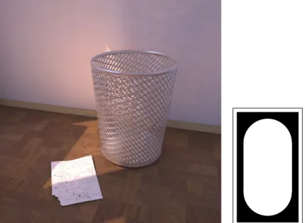
used and0where no surface should be. Figure 2.6 illustrates the use of a clip map on
Figure 2.6: Clip Mapping on a trash can. The trash can was modeled from a cone and a clip map was used to create the mesh structure. The clip-map is shown on the right. Note that the torn out corner of the paper on the floor was also modeled with a clip map.
These kind of textures are special because they can be interpreted to not modify the shader but instead to modify the underlying geometry. They could, of course, be implemented as a shader. This but then the shader is responsible for creating a new ray when the surface is clipped away. Considering high performance ray tracing this is inefficient since a lot of overhead is involved in creating a new ray and starting a new traversal at the root node. Instead it is much more efficient to integrate clip maps directly into the ray tracing core. This has to be considered when designing a ray tracer for a full rendering system. To enable a ray tracing core to directly use clip mapping the information has to be accessible during the triangle intersection computation. This adds an additional conditional in the triangle intersection computation to check if a clip map is attached to the triangle and then check if the intersection is clipped away. This direct integration is not as trivial as it may seem as, depending on the ray tracing system, the texture coordinate computation and access can be quite complicated. This leads to a design choice on how tightly coupled the ray tracer should be with the rendering system. For our ray tracing system developed in this thesis that was used for example to create the image in Figure 2.6 we added support for simple1-bit clip maps directly to
2.3.4 Material Representation
When talking about materials for rendering systems there are two concepts that need to be distinguished. The first is the bi-directional reflectance distribution function (BRDF) which is usually a mathematical model for describing the reflection behavior of a sur-face. An alternative to a mathematical model is to use measured data ([Matu 03]). The other concept is usually called a shader. A shader can be a complex program where the behavior is fully programmable by the artist. While in a general artistic rendering system this freedom poses no major problem for the rendering algorithms it has to be more restricted in the context of physically based rendering. Here we use the notion of a shader as a group of BRDF with the parameters for this models included. The BRDF are fixed in our context but the parameters (for example the diffuse color) may be programed or read from a texture. An important fact is that the material model used in a rendering system has a significant impact on the correctness and on the rendering speed. There have been a lot of BRDF models proposed that fulfill the requirements of a Monte Carlo rendering system. For correct results the BRDF has to be energy conserving and needs a representation that allows for efficient evaluation as well as for the ability to importance sample it effectively. This is in contrast to a generic shader that is used in a more general rendering application. Usually a BRDF model is part of such a shader but does not need to obey the energy conservation. In our system we can use any of the physically based BRDF models that were developed like the one by Schlick [Schl 94] or Ward [Ward 92a].
A physically based BRDF model is defined as a function f(x, ωi, ωo) :=
dLr(x, ωo) dEi(x, ωi)
that depends on the quotient of the reflected radianceLrat a given surface-pointxand
the outgoing directionωo and the incident irradianceEiat the same surface point from
incoming directionωi. It is used in the integral of the rendering equation 6.1.
In Section 2.3.4 we develop a small extension to the reflection model described in [Blin 77] that is designed to provide all the needed functionality for a flexible material system and is perfectly suited for the rendering algorithm we describe.
Each BRDF model can have many different parameters to tune it’s appearance. These parameters can be set for each object but more commonly they are set using texture maps on objects. To support different parameters like diffuse color, different kinds of exponents, specular color etc. the system has to provide the ability to use mul-tiple texture maps per object. This is easy to implement but has to be considered in the data format as it is often needed to provide different parametrizations (called uv sets) for each texture.
A Simplified Practical Layered Material Model
Here we will describe shortly the material model we use in our rendering system. It is especially developed for the use in the path space partitioning method in Section 6.3
but is general and we use it for all of our algorithms.
While general production renderers for the movie industry can use arbitrary and complex programs to define surface color and reflection behavior [Drie 05, Kess 08], physically-based systems are more restricted in their choice of reflection functions [Phar 04]. Many practical algorithms exploit the fact that BRDFs are not only energy-conserving, but also provide an efficient sampling function.
A wealth of surface reflection models have been developed in computer graphics that provide most of the required functionality [Blin 77, Ward 92a, Ashi 00]. These reflection models allow one to describe a wide variety of basic surface types. For more complex surface behavior usually several reflection models are combined to a single layered material [Phar 04]. Physically based rendering systems require the BRDF model to satisfy the Helmholtz reciprocity condition in order to obtain consistent results. The renderer we develop in Section 6.3 partitions path space and uses only one technique on each partition, therefore this condition no longer needs to be fulfilled, allowing us to use more convenient approaches like e.g. the halfway vector disc model [Edwa 06] or even arbitrary programs for surface shading.
In order to determine the partition of the path space, we need to decide when a reflection is almost diffuse. In principle our system can use any physically-based layered BRDF model for which a parameterκ can be assigned to each layer expressing how diffuse it is. This parameter is assumed to be normalized such that forκ= 0the layer is
perfect Lambertian and forκ= 1the surface is a perfect mirror. During rendering each
sample evaluates only one material layer that is selected by random sampling. We use the threshold ofκ= 0.2for classifying a material layer as diffuse or specular.
For example, in all renderings we use the Blinn-Phong model [Blin 77] with Phong-exponent k = 1024κ + 1. Layered materials such as simple metal or glass (one
re-flecting, one transmitting layer) and more complex materials like coated plastic can be constructed easily using the Fresnel term or one of the approximations [Schl 94] for weighted sampling of material layers. For transmissive materials the direction is se-lected according to Snell’s law but the width of the lobes is controlled as before, as this allows for diffuse and imperfect glass.
The common approach in a physically based rendering system is to support multiple different material models that are all combined using a standardized sampling interface. This approach allows the artist using the rendering system to freely choose appearance and also allows for plug-in materials. While this increases the flexibility of the rendering system it comes at the cost of more complex scene construction and has a high impact on the rendering speed. Additionally supporting plug-in materials is problematic in the context of physically based rendering because it requires the plug-in author to imple-ment a mathematically correct BRDF model. The speed impact results mostly from the need for a general interface inhibiting pre-computation of parameters and making SIMD processing of the material model difficult.
In contrast to the common method of supporting multiple different material models we propose a simple physically correct material model with layering. Multi layered materials are a natural choice for progressive rendering. In a progressive renderer not all layers
need to be evaluated at once but can be sampled according to their weight. For example the Ashikmin-Shirley BRDF model ([Ashi 00]) is an implicit multi-layered material model with two layers, a diffuse and a specular. The obvious advantages of a single material model are that each surface behaves the same (at least within the parameters of the shading model) and a single optimized code path can be used. It also simplifies SIMD optimization of the code.
In our model we use multiple layers of the energy corrected Blinn-Phong model that was presented in [Blin 77]. Each layer is a weighted instance of this basic model. Dur-ing samplDur-ing a random variable is used to choose between these layers and potential absorption. This variable is also used to sample whether the transmissive part of the material should be sampled (using the Fresnel term of this layer). Each layer has two color channels (called C0 and C90) that are interpolated based on the Fresnel term.
This is an artistic extension to the classical wavelength independent Fresnel term that always approaches a value of1at gracing angles. This behavior is a special case of our
method by setting each channel inC90 equal to1. The effect of this parameter is
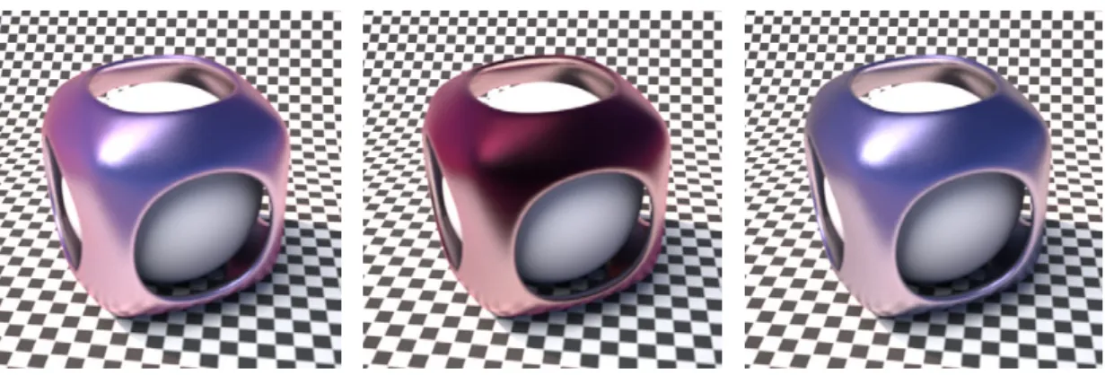
illus-trated in Figure 2.7. With the use of the color interpolation reciprocity is of course lost for this BRDF model, but with our path space partitioning described in Section 6.3 this is not a problem. To control the specular behavior each layer has a parameter called hardness (κ) that varies from0.0(Lambertian) to1.0for a perfect mirroring layer.
Figure 2.7: Visualization of using the Fresnel term to interpolate between two colors. The left image shows the interpolated results. The middle image hasC0 = 0
and the right image hasC90 = 0. Note the difference in the highlights from
the sun and the slightly different position.
In the following we describe the material model used for each layer in our system. As already mentioned above we use the Blinn micro-facet distribution with the additional normalization needed for physically based rendering.
fr(x, ωi, ωo) =
hn, hik·k+2 2
4πhn, ωoihh, ωoi
(2.1) The exponent k is computed from the hardness value κ specified for each material
ωh
ωo
n
ωi
Figure 2.8: The directions and vectors used for the BRDF computation of a single layer.
layer. A practical value to map the interval ofκ ∈ (0,1)to the exponent k is given by k = 1024κ+ 1. There are two special cases of this BRDF for κ = 0 and κ = 1. In
the case of κ = 0 a Lambertian layer is constructed and forκ = 1 a perfect mirror is
assumed. Note that equation 2.1 does not produce itself a Lambertian BRDF forκ→0.
Figure 2.9 illustrates the effects of this parameter for a single layer material model.
Figure 2.9: Varying the hardness from0.0to1.0for a single layer material.
To edit these materials we implemented an easy to use material editor that integrated the full renderer to preview the parameters. Figure 2.10 shows two screenshots of this editor. Since the material model is very simple the functionality depicted in these two screenshots is already enough to create a wide variety of realist materials that work with our rendering system. Two materials are illustrated in Figure 2.11.
2.3.5 Sampling Light Sources
For almost all global illumination algorithms, the rendering system has to be able to generate correctly weighted sample points on light sources. As we consider only
phys-Figure 2.10: The Material Editor developed for the layered BRDF described above shows the simplicity of the model. The two screen-shots already describe the full functionality needed.
Figure 2.11: Two example renderings illustrating realistic materials created with our ma-terial model. The left shows a glass mama-terial and the right a multilayer car paint material.
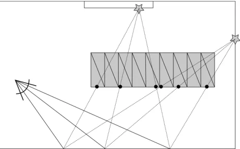
ically plausible scenes in our rendering system, light sources (with the exception of environment maps) are part of the scene and modeled as triangles. These triangles are marked as emitters and have the light source information like spectral properties and emittance behavior. The usual way to generate sample points on light sources is to build a cumulative density function (CDF) using the emittance power of each triangle. Now three random or quasi-random numbers are needed to select a triangle and a point on this triangle. This approach works well if all light sources in the scene contribute to the final image. Since the CDF is build based on the power, bright light sources are sampled more often than dark light sources. The problem with this approach is a dra-matic decrease in efficiency when larger scenes are rendered. For example a complete modeled house has many light sources but the camera is only in a single room. An
ap-proach in unbiased rendering algorithms is to build the CDF based on the light source contribution to the final image [Sego 06].
This can work well but needs many light samples until a good CDF is acquired. This many light samples are not available when directly using only point light sources. An-other problem with this method is, that it can’t be used when the scene is illuminated by a sky model ([Pree 99]) or when image based lighting ([Debe 98]) is used.
We develop an approach completely based on the usage of point light sources that works also well when image based lighting and other environment illumination is used by discarding unimportant light sources stochastically. This approach is described in Section 6.3.2. A full rendering system also needs to support image based lighting using environment maps. In Section 6.4 we will present a physically correct solution on how to integrate infinitely far away illumination with a point light based rendering system.
2.4 Processor Architecture
In light transport simulation there are a few core algorithms that will be executed a million times or more and will amount to over 90% of the computation time. For this reason even small optimizations to these core algorithms are beneficial for the final rendering speed. So after considering all algorithmic optimizations it is important to directly optimize for the target processor architecture. Additionally, the shift in processor architecture has to be also recognized by algorithm design. Simply using classical algorithms on modern architectures does not give the performance the new hardware promises.
This shift in processor architecture consists mainly of two trends. The first one is an increase in the number of processing elements and the number of instructions that can be executed in parallel. Multi-core and many-core are almost ubiquitous and addition-ally the increasing availability of chip area allows to pack multiple computation pipelines and execution units into the CPU. This results in different parallelizations that are avail-able to the programmer that have to be recognized when designing algorithms. At one end are multiple full processor cores that are able to execute independent streams of instructions. On a lower level there are SIMD (single instruction multiple data) units that allow to execute a single instruction on several data elements. SIMD is explained in more detail below. The most common size for SIMD units is currently 4 but in the
future much wider SIMD-width are to be expected [Seil 08]. Further forms of parallel execution can be found in multiple execution units that allow for example to execute a memory fetch and a computational instruction in parallel at the same time. Usually on this low level a programmer expects the compiler to know the underlying architecture and optimize for it. But a knowledge of this behavior aids algorithm design. Knowing for example that a computation between memory fetches is virtually free may change the design significantly. The second trend in processor architecture can be explained by the divergence of computation speed and memory access time. This leads to either deeper and large caches or different memory models that require coherent memory access.
For maximum performance each new architecture and the trade-offs have to be re-considered. Thus partitioning the ray tracing algorithm into several distinct parts makes it easier to understand the problems and to find fitting solutions for the chosen hardware platform.
It is likely that the upcoming computer architecture for commodity hardware become even more heterogeneous than it is today. Several different computational engines will be found in the usual desktop computer. Aside the graphics processing unit with it’s ever increasing power there exist affordable acceleration cards for Physics Simulation or more general acceleration cards like an additional CELL processor on an PCI-Express card. Even inside a single architecture like the CELL-Processor a heterogeneous col-lection of two different computational engines can be found.
This heterogeneous hardware allows one to spread the computation over different processors and a first approach to use it would be to use the computational engine that is best suited for the given task. Another goal could be to use all different available computational engines to solve a given task as quickly as possible. In that case it may be an enormous task for the application developer to efficiently use all different engines at the same time without stalls.
In the following we shortly review some important architectural topics that later in this thesis guided the design decisions and may be required to understand some of the op-timizations. More details are given when needed in the specific sections. In this thesis we are mainly concerned with accelerating ray tracing on general purpose processors that can be found in any desktop computer or notebook. In the last few years an in-creasing amount of research has been done to bring ray tracing to graphics processing units (GPUs) and their unique architecture. While these are quite successful and pro-vide sometimes much higher speed there are still some limitations that restrict the use of these ray tracers in a fast full global illumination renderer. One problem is for exam-ple the limited amount of memory these graphics cards have in many cases. Another problem is that complex shading operations are solved mostly in a hybrid approach and can not fully utilize the advantages of GPUs. There is still a lot of ongoing research to create systems that efficiently use the graphics cards. Most of the results we present in the next section can be employed to any ray tracer regardless on which hardware it runs on. But some design considerations especially for the novel acceleration structure we present in Section 3.2 is specifically targeted towards CPU architectures. We want to note here again that we are mostly concerned with accelerating incoherent rays that occur in global illumination computations. These are very troublesome for all GPU ray tracers that usually slow down to speeds comparable to CPU ray tracers. Only recently some hardware modifications to allow GPUs to trace faster incoherent rays have been presented in [Aila 10] but these are still only theoretical.
Parallel Processing
There exist a lot of different parallel architectures and several programming models that can be used to parallelize a given problem. A very good introduction to parallel
pro-gramming can be found in [Quin 03]. On the usual multi-core (CPU) machines a ray tracing based image generation algorithm is rather easy to parallelize once the acceler-ation structure has been build. The parallel construction of acceleracceler-ation structures is an interesting problem and has for example been investigated forkd-trees in [Ize 06] or for bounding volume hierarchies in [Laut 09]. Each core may have it’s own caches but they all access the same main memory. Since each ray is at first independent of each other ray they can be traced in parallel and only the final combination in the frame buffer has to be synchronized. On NUMA (Non-Uniform Memory Architecture) machines building a scalable solution is more difficult. A possible solution strategy for the visualization of larger models is described in [Step 06].
Intrinsics. To really utilize a given hardware architecture the written code needs low level access to all available functions. Many complex operations are often available as a single CPU instruction but it may not be possible to express this directly in a high level language. Still, for developing high performance algorithms it is not necessary to directly program in the assembly language of the processor. High level language compilers like many C and C++ compilers provide a mechanism calledintrinsics that allow to access specific instructions directly from within high level code. These intrin-sics are implemented by many compilers as extensions to the language standard. For example the usage of intrinsics for the Intel compiler is described in [Scho 03] and the GCC is compatible to the intrinsic usage for Intel platforms. Intrinsics not only allow to perform specialized instructions on registers and memory regions but also can ac-cess for example hardware counters or control the cache acac-cess and pre-fetching. But they are of course specific to a given hardware. This has the disadvantage of reduced portability. Each different hardware platform from another vendor has its own set of in-trinsics. Hardware from a single vendor is usually backwards compatible but introduces new functions with each release. Still the benefit of using intrinsics is too large to be ignored, especially for SIMD processing described in the next Section. To support mul-tiple platforms we will develop and use a simple abstraction layer described also in the next Section.
SIMD Processing. SIMD is an acronym that stands for Single Instruction Multiple Data. It is a form of parallelism where multiple streams of data are processed by a single stream of instructions. A processing width of4then means that 4 data elements
are processed by a single instruction in parallel. This is illustrated in Figure 2.12 for two simple operations.
Often the number of data elements is not directly fixed but the width of a single pro-cessing element. A common size are128-bit registers and all SIMD instructions operate
on this width. In a128-bit register fit for example four32 bit floating point numbers or
integers or16 8-bit chars.
Almost all modern hardware architectures provide hardware support for SIMD pro-cessing each with its unique marketing brand name. The companiesIntel and AMD
3 5 2 8 12 9 6 11 A0 A1 A2 SIMD ADDA2, A0, A1 + 3 6 1 9 SIMD CLEA2, A0, A1 3 2 9 0 0 -1 -1 A0 A1 A2 ≤ 5 3 6 1 7
Figure 2.12: Illustrating the principle of SIMD computation. The first instruction is a sim-ple add. Adding two SIMD registers results in a component wise addition. The second instruction is a compare for less or equal. This is again done component wise. The result of a comparison is 0 when it is false. When
the comparison results in true each of the bits in the component are set to
1. This is the binary integer representation of −1. The reason for setting
all bits to1is that the result can now be easily used in masking operations
by using bit-wiseand andor operations.
now support the SSE instruction set (where various different versions exist). The In-tel SSE instruction set is described in detail for example in [Inte 09]. The older SIMD instructions sets that are still supported areIntel MMX andAMD 3dnow. Sun has the MAJC architecture,IBMhas Altivec for the PowerPC and CELL SPE [Cell 09] architec-ture,ARM names it NEON [Cort 09], and for the SPARC architecture it is called VIS.
All these processing units are vendor-specific and provide different functionality with no unified or standardized way to program them. The usual way to develop for them in a high level language is to use intrinsics but they are also platform dependent. Luckily even though the used instructions may differ in details, many of the standard opera-tions have equivalents on most other architectures. So, for example, a SIMD width of
4 (currently the standard on almost all CPUs) and the basic operations like addition,
multiplication and bit wise operations are available everywhere. This allows one to use a simple and basic abstraction layer building a wrapper around the intrinsics. For the use in this thesis we developed a simple collection of C pre-processor macros that has a back-end for PowerPC Altivec, Intel SSE and a software implementation for comput-ers without SIMD instruction set and for debugging purposes. Instead of pre-processor macros inline functions could also be used. This abstraction can easily extended to support other SIMD vector units of the same size. It is important to note that the ab-straction should be as close as possible to the underlying hardware as else many of the low level optimizations could not be implemented.
In the following we present the basic ideas by presenting the implementation of some selected functions. This also serves as an introduction to SIMD programming. The first step is to define a type for the basic most commonly used data types. In the case of a ray tracing based image generation software the most basic types are a 32-bit integer
# i f d e f USE_ALTIVEC
typedef v e c t o r f l o a t SIMD_float ; typedef v e c t o r i n t SIMD_int ; # e l i f definded (USE_SSE)
typedef __m128 SIMD_float ; typedef __m128i SIMD_int ; # else
typedef union ALIGN16 SIMD_float { f l o a t ALIGN16 f [ 4 ] ;
unsigned i n t ALIGN16 i [ 4 ] ;
} ALIGN16 SIMD_float ;
# e n d i f
Listing 2.1: Data structure definition for the SIMD abstraction code.
and 32-bit floating point numbers. For the software implementation a union is used
because of the ability of all vector units to interpret the contents of a register without conversion. On PowerPC there exist a language extensions for vector units that uses overloaded operations. So for example for an addition no direct intrinsic is needed and the add operator+can be used.
Now implementing the basic arithmetic and logic functions is straightforward. List-ing 2.2 shows as an example the implementation of two arithmetic instructions for the SIMD abstraction layer. The Altivec version can use the overloaded operator, the SSE version uses intrinsics and the non vectorized version modifies each component indi-vidually. Note that the compiler automatically unrolls theforloops in this case.
The last example shown in Listing 2.3 is more complex and illustrates the possibility to support instructions that are not equal over different architectures efficiently. Here we chose the SSE shuffle instruction that is needed for example for the SIMD sorting used in Section 3.3.3. Luckily the permutation function of Altivec units is able to perform the operations of an SSE shuffle instruction. The shuffle instruction is best understood by looking at the software implementation in Listing 2.3. The goal is to reorder the4
elements in an SIMD register by providing its new positionsa, b, c, d. For the SSE version there exist a macro in the SSE API_MM_SHUFFLE(...) that constructs the re-quired bit mask for the_mm_shuffle_psinstruction. The Altivecvec_perminstruction is more powerful than required but with a simple look-up table the workings of the shuffle instruction can be mapped. This is of course non-optimal considering the Altivec archi-tecture as more instructions are needed but in our application the shuffle instruction is only a small part of the algorithm and it does not hurt the performance much compared to the fact that the same code can be used on all platforms. Some of the modern com-pilers have the ability for auto-vectorization. This can, in theory, automatically generate SIMD code from the program code but works only in very few cases. So manual written code is still far superior to compiler generated SIMD code for complex algorithms.
# i f d e f USE_ALTIVEC # d e f i n e SIMD_ADD( a , b ) ( ( a ) + ( b ) ) # d e f i n e SIMD_CLE( a , b ) ( ( v e c t o r f l o a t) vec_cmple ( a , b ) ) # e l i f definded (USE_SSE) # d e f i n e SIMD_ADD( a , b ) ( _mm_add_ps ( a , b ) ) # d e f i n e SIMD_CLE( a , b ) ( _mm_cmple_ps ( a , b ) ) # else
s t a t i c i n l i n e SIMD_float SIMD_ADD( SIMD_float a , SIMD_float b ) {
SIMD_float r ; f o r (i n t i = 0; i < 4; i ++) { r . f [ i ] = ( a . f [ i ] + b . f [ i ] ) ; } r e t u r n r ; }
s t a t i c i n l i n e SIMD_float SIMD_CLE( SIMD_float a , SIMD_float b ) {
SIMD_float r ; f o r (i n t i = 0; i < 4; i ++) { r . i [ i ] = ( a . f [ i ] <= b . f [ i ] ) ? −1 : 0; } r e t u r n r ; } # e n d i f
Listing 2.2: Basic arithmetic instruction macros for the SIMD abstraction layer. The in-structions are an addition (ADD) and a comparison for less or equal and are explained in Figure 2.12.
Memory
Increasing the number of cores not only poses new problems for the algorithm design but also increases the well known problem of the divergence of memory access speed versus compute power. While in the last years the compute power has almost increased exponentially according to Moore’s law1 the memory access speed has grown only
linearly. This gap is well known and one of the common solutions to alleviate this is by the introduction of cache hierarchies. The basic idea here is to introduce additional memory blocks that are smaller but are located closer to the CPU and thus can be accessed faster. A very good and complete treatment of the memory subsystem and caches in modern commodity hardware can be found in the technical report by Drepper [Drep 07]. In the following we just review the aspects that are directly important to the optimization considerations developed in this thesis.
At first, a programmer has to be aware of the existence of caches or their absence. For example on the CELL architecture or on GPUs there may be no hardware caching for some of the memory accesses but local memory that is programmer controlled. In these cases a software managed cache is often a viable alternative. Directly
consid-1Actually Moore’s low only states that the number of transistors roughly doubles every two years, but due
to ever improving hardware designs and on-chip parallel processing like SIMD this directly relates to the raw compute power of a CPU.
# i f d e f USE_ALTIVEC
s t a t i c const unsigned i n t _av_shufmask [ ] = {0 x00010203 , 0x04050607 ,
0x08090A0B , 0x0C0D0E0F , 0x10111213 , 0x14151617 , 0x18191A1B , 0x1C1D1E1F } ; / / S h u f f l e Semantic : c , d , e , f i n [ 0 , 3 ] ( SSE−S t y l e )
/ / e , f are l o w e r ; e , f s e l e c t from a / / c , d are upper ; c , d s e l e c t from b
# de fi ne SIMD_SHUFFLE( a , b , c , d , e , f ) (
vec_perm ( a , b , ( v e c t o r unsigned i n t) { _av_shufmask [ f ] , _av_shufmask [ e ] ,
_av_shufmask [ d +4] , _av_shufmask [ c + 4 ] } ) ) # e l i f definded (USE_SSE) # de fi ne SIMD_SHUFFLE( a , b , c , d , e , f ) ( _mm_shuffle_ps ( a , b , _MM_SHUFFLE( c , d , e , f ) ) ) # else
s t a t i c i n l i n e SIMD_float SIMD_SHUFFLE( SIMD_float f1 , SIMD_float f2 , i n t a , i n t b , i n t c , i n t d ) { SIMD_float r ; r . f [ 0 ] = f1 . f [ d ] ; r . f [ 1 ] = f1 . f [ c ] ; r . f [ 2 ] = f2 . f [ b ] ; r . f [ 3 ] = f2 . f [ a ] ; r e t u r n r ; } # e n d i f
Listing 2.3: Implementation of the SIMD shuffle instruction for the abstraction layer. Shuffle reorders the4elements of an SIMD register. The Altivecvec_perm
instruction is more powerful than the SSE counterpart as it allows re-ordering and replication of individual bytes. This explains the lookup-table
_av_shufmask.
ering a cache hierarchy in an implementation means to fit the data types and memory accesses to the cache line width and the access structure of the main memory. The next thing to consider is the latency of a memory access. This latency of course varies greatly on where the requested data is currently stored in the cache hierarchy. Knowing this latency may allow an algorithm to run faster by reordering for example the instruc-tions in a way that after a memory request other independent computainstruc-tions can be performed. Usually a modern compiler tries to optimize given code in a way fitting to the hardware but it can only use information locally available. A programmer has ap-plication domain knowledge and information about the actual execution behavior of an algorithm that allows even better optimization2.
A rather old technique to hide some of the memory access latency is called simulta-neous multi-threading [Tull 95]. Intel implemented the technique [Marr 02] in hardware and called it hyper threading. This technique basically allows to switch executing
an-2Modern compilers support profile guided optimization that allows to run an instrumented version of a
program to automatically gather run-time information that is used in a second compilation step for further optimization
i n t value ; i n t∗ p = &value ; p = p | 2; / / s t o r e some i n f o r m a t i o n i n t h e l a s t two b i t s . . . i f ( p & 3 == 2) { . . . / / do s t h . w i t h t h e i n f o r m a t i o n s t o r e d . . .
i n t number = ∗( p & 0xFFFFFFF7 ) ; / / access t h e o r i g i n a l v a l u e
Listing 2.4: Bit Operations to use the two unused bits in a memory address to store and retrieve information. This is for example useful when storing child pointer in acceleration structures.
other stream of instructions when a high latency memory access occurs. Simultaneous multi-threading can also be implemented in software and is a common approach to hide DMA latency for example on CELL architectures [Cell 09].
Instead of manually optimizing algorithms to a specific memory hierarchy and caching structure there exists another approach called cache oblivious algorithms. An overview can be found in chapter 38 of the “Handbook Of Data Structures and Applications” [Meht 04]. While not achieving peek performance they can make some algorithms more portable across multiple platforms and still provide high performance. But of course they can not adapt to situations like the CELL architecture where no caches are available at all. Nevertheless these methods can be directly applied to computer graphics related problems like mesh layout [Yoon 05] and for bounding volume hierarchies [Yoon 06]. Low Level Operations
Programming close to the underlying hardware is important in getting the last bit of performance out of a given algorithm. Additionally knowing the exact size and bit layout of data types allows to efficiently use all available bits. In this section we review the important data types and standard approaches that are used during optimization. A very good and helpful book about optimizing computations using the benefits of the binary number representation in a computer is [Warr 02].
Bit Operations. When optimizing algorithms it is often beneficial to use every last bit in a memory region. Especially when memory access is optimized collecting all infor-mation in a small space reduces the number of memory accesses and cache thrashing. For example the standard size of an integer or floating point number is currently4bytes.
For alignment reasons a memory location for such a number is divisible by4. So when
a pointer to this memory address is stored that last two bits are always 0. Knowing
this, it is easy to store up to 4different additional states by using a bit-wise or. Using
this method it is necessary to mask these two bits before using the variable for memory access. The small code section in Listing 2.4 shows an example usage on32bit
2 Image Generation Fundamentals
1 8 23
sign exponent mantissa
Figure 2.13: Bit layout of an IEEE32-bit floating point number.
structure for ray tracing where for example the split axis of akd-tree node (3 possible
choices in 3d) can be stored in a memory pointer. The last state can be used to indicate a leaf node.
Floating Point Representation. The IEEE 754 standard [IEEE 85] for floating point numbers (floats) is widely adopted now by processor manufacturers. Nevertheless many vendors only implement a subset of the full standard for performance and die area reasons. For example it is common to omit the support for denormalized numbers or only provide a subset of the standardized rounding modes. Sometimes the accuracy may also vary but the general representation of a floating point number is still the same across a wide range of platforms. An introduction to the use of floating point numbers in scientific applications is given by Goldberg in [Gold 91]. The general layout of a32-bit
floating point number is illustrated in Figure 2.13. As32-bit floats provide in many cases
enough accuracy for graphics application and they are the only ones considered here. Looking at the bit representation of a floating point number we can use some of the bits for other purposes when we know something about the stored number. For example when we know that the number is always positive we can use the first bit in the floating point number. When we know that an absolute value of a number is always smaller or equal to 1, a single bit in the exponent is free (This is for example the case when
storing normal vectors or RGB-float colors). When not the full accuracy of the 23-bit