ISSN 2042-2695
CEP Discussion Paper No 1024
November 2010
Do Matching Frictions Explain Unemployment?
Not in Bad Times
Abstract
This paper models unemployment as the result of matching frictions and job rationing. Job rationing is a shortage of jobs arising naturally in an economic equilibrium from the combination of some wage rigidity and diminishing marginal returns to labor. During recessions, job rationing is acute, driving the rise in unemployment, whereas matching frictions contribute little to unemployment. Intuitively, in recessions jobs are lacking, the labor market is slack, recruiting is easy and inexpensive, so matching frictions do not matter much. In a calibrated model, cyclical fluctuations in the composition of unemployment are quantitatively large.
Keywords: Unemployment; matching frictions; job rationing JEL Classifications: E24, E32, J64
This paper was produced as part of the Centre’s Macro Programme. The Centre for Economic Performance is financed by the Economic and Social Research Council.
Acknowledgements
I am deeply indebted to George Akerlof and Yuriy Gorodnichenko for their invaluable advice, continuous guidance, encouragement, and support. I am extremely grateful to Bob Anderson, Andy Atkeson, David Card, Thomas Chaney, Urmila Chatterjee, Varanya Chaubey, Pierre- Olivier Gourinchas, Christian Hellwig, Chad Jones, Shachar Kariv, Patrick Kline, Botond Köszegi, Maciej Kotowski, David Levine, Lars Ljungqvist, Juan Carlos Montoy, Kristoffer Nimark, Maury Obstfeld, Demian Pouzo, Matthew Rabin, Emmanuel Saez, Robert Shimer, David Sraer, Mike Urbancic, Thijs Van Rens, and especially David Romer, who contributed valuable comments and suggestions at different stages of this project. I have also greatly benefited from comments received in various seminars.
Pascal Michaillat is an Associate of the Macro Programme at the Centre for Economic Performance and Lecturer in Economics, London School of Economics.
Published by
Centre for Economic Performance
London School of Economics and Political Science Houghton Street
London WC2A 2AE
All rights reserved. No part of this publication may be reproduced, stored in a retrieval system or transmitted in any form or by any means without the prior permission in writing of the publisher nor be issued to the public or circulated in any form other than that in which it is published.
Requests for permission to reproduce any article or part of the Working Paper should be sent to the editor at the above address.
1
Introduction
Unemployment spikes frequently across the U.S. and Europe, most recently in 2008–2010, and remains a major concern for policymakers. To determine optimal policy responses, it is critical to identify the main sources of unemployment. I propose a framework that accommodates two important sources of unemployment: (i) job rationing, which is a shortage of jobs in the economy; and (ii) matching frictions, which make it costly for recruiting firms to match with unemployed workers. I study how these two sources interact over the business cycle to shed new light on the mechanics of unemployment fluctuations.
This paper develops a tractable model that distinguishes between two components of unemploy-ment: (i) rationing unemployment, which measures the shortage of jobs in the economy, irrespec-tive of matching frictions; and (ii) frictional unemployment, which measures additional unemploy-ment attributable to matching frictions. Formally, I define rationing unemployunemploy-ment as the amount of unemployment that would prevail if recruiting cost was zero, and frictional unemployment as additional unemployment due to a positive recruiting cost. The paper makes four contributions to our understanding of unemployment fluctuations. First, it proposes conditions under which ra-tioning unemployment is positive. Second, it proves theoretically that during a recession rara-tioning unemployment increases, driving the rise in total unemployment, while frictional unemployment decreases. Third, it shows that even a small amount of wage rigidity, such as that estimated with microdata on earnings of newly hired workers, is sufficient to amplify technology shocks as much as in the data. Hence, moments of key labor market variables simulated with the calibrated model match those estimated in U.S. data well. Fourth, the paper finds that cyclical fluctuations in the composition of unemployment are quantitatively large: when unemployment is below 5 percent, it is all frictional; but when unemployment reaches 8 percent, frictional unemployment amounts to less than 2 percent of the labor force, and rationing unemployment to more than 6 percent.
The model departs from the literature by allowing for job rationing, a shortage of jobs resulting from a failure of the labor market to clear even in the absence of matching frictions. Even if re-cruiting cost is zero, workers may not all be profitably employed and some unemployment, which
I call rationing unemployment, may remain. Since recruiting cost is actually positive, total unem-ployment is higher than rationing unemunem-ployment, and the difference between the two is frictional
unemployment.
There is no job rationing in existing search-and-matching models because they assume that there would not be any unemployment without a positive recruiting cost. In the canonical search-and-matching model, wages are the outcome of Nash bargaining and by construction always remain below the marginal product of labor (Hagedorn and Manovskii 2008; Mortensen and Pissarides 1994; Pissarides 2000; Shimer 2005). Therefore if recruitment cost falls to zero, firms make a positive profit on each new match and will enter the labor market until there is full employment. By the same logic, there is full employment in the absence of recruiting costs in models using different bargaining procedures (Cahuc et al. 2008; Elsby and Michaels 2008; Hall and Milgrom 2008;Rotemberg 2008). Shimer(2004) andHall(2005a) introduce wage rigidity into search-and-matching models, in the form of a constant real wage. But since these models assume atomistic firms for simplicity, the marginal product of labor is independent of aggregate employment. Thus if productivity is above the constant wage and recruitment cost falls to zero, firms enter until there is full employment. Job rationing is absent from these atomistic-firm models with rigid wages, and likewise from large-firm models with wage rigidity and either constant marginal returns to labor in production, or diminishing marginal returns to labor and instantaneous capital adjustment (Blanchard and Gal´ı 2010;Gertler and Trigari 2009).
To provide a more general framework in which unemployment may arise from both matching frictions and job rationing, this paper builds on the Pissarides(2000) model by relaxing two of its key assumptions: completely flexible wages and constant marginal returns to labor. These assumptions are critical because either implies that there would not be any unemployment without a positive recruiting cost. Specifically, I develop a dynamic stochastic general equilibrium model in which large firms face a labor market with matching frictions, as inBlanchard and Gal´ı(2010). All household members are in the labor force at all times, either working or searching for a job. Firms open vacancies to hire new workers each period in response to exogenous job destruction and technology shocks. Recruiting is costly because of matching frictions, especially in expansions
when firms post many vacancies that are filled from a small pool of unemployed workers. I assume that firms face diminishing marginal returns to labor in production. I introduce rigid wages, which do not adjust as much as technology. In a frictional labor market, rigid wages are a possible equilibrium outcome. Even if wages are rigid, they may remain in the interval between the flow value of unemployment and the marginal product of labor, and neither interfere with the efficient formation of worker-firm matches nor cause inefficient match destructions. In that case, wages satisfy the equilibrium requirement that worker-firm pairs exploit all the bilateral gains from trade (Hall 2005a).
Assuming diminishing marginal returns to labor and wage rigidity is appealing for several rea-sons. First, both assumptions have been used (but not combined) in the search-and-matching lit-erature, and are standard in the broader macroeconomic literature.1 Second, both are empirically relevant. At business cycle frequency, some production inputs are slow to adjust and the short-run production function is likely to exhibit diminishing marginal returns to labor. Substantial ethno-graphic and empirical literatures also document wage rigidity.2Third, job rationing can be readily quantified, because diminishing marginal returns to labor can be calibrated using aggregate data on the labor share, and the response of wages to technology shocks has been estimated with microdata on individual wages.
The fundamental property of this model is that there may be some unemployment even in the absence of matching frictions. To understand why jobs may be rationed, I first abstract from re-cruiting expenses. Since there is perfect competition in the goods market, firms hire workers until marginal product of labor equals wage. The marginal product of labor decreases with employment because of diminishing marginal returns. In response to a negative technology shock, the marginal product of labor falls whereas rigid wages adjust downwards only partially. If the shock is
suffi-1There is a long tradition of macroeconomic models featuring a short-run production function with labor as the only variable input, and with diminishing marginal returns to labor (for example,Benigno and Woodford 2003). Wage rigidity features in the many dynamic stochastic general equilibrium models that use theTaylor(1979) and Calvo
(1983) staggered wage-setting mechanisms, and Christiano et al. (2005) argue that wage rigidity is important for improving realism in this class of models.
2Blinder and Choi (1990), Campbell and Kamlani (1997) and Bewley (1999) provide ethnographic evidence. Kramarz(2001) surveys studies based on wage microdata. Dickens et al.(2007) provide recent evidence from Eu-ropean wage microdata.
ciently large, the marginal product of labor of the last workers in the labor force may fall below the wage. It becomes unprofitable for firms to hire these workers. Some unemployment, which I call rationing unemployment, would prevail even if recruiting cost was nil. With a positive recruiting cost, the marginal cost of labor is higher and firms reduce employment. The resulting amount of additional unemployment is frictional unemployment.
In recessions marginal profitability falls further and job rationing is more acute. Rationing unemployment increases, driving the rise in total unemployment. Many unemployed workers apply to the few vacancies left. Each vacancy is filled rapidly and at a low cost in spite of matching frictions. Since recruiting expenses barely raise the marginal cost of labor, profit-maximizing firms barely reduce employment compared to the level prevailing in the absence of recruiting costs. Therefore, frictional unemployment is lower in recessions than in normal times. To summarize, in expansions, matching frictions explain all of unemployment. In recessions, falling technology leads to an acute shortage of jobs that drives an increase in total unemployment; simultaneously, the amount of additional unemployment attributable to matching frictions falls because it becomes easier for firms to recruit.
I commence the analysis with a theoretical study of the comovements of unemployment and its components using comparative statics with respect to technology. I opt to work in a model without aggregate uncertainty because it has the same qualitative behavior as the fully dynamic model, in spite of the dynamic nature of firms’ decisions and the dynamic adjustment process of unem-ployment. Moreover its equilibrium can be studied analytically and represented diagrammatically. Next, I use numerical methods to quantify frictional and rationing unemployment in a stochastic environment that accounts fully for rational expectations of firms as well as the law of motion of unemployment.
I calibrate the model with U.S. data and simulate the impact of technology shocks. Simulated moments for labor market variables are close to their empirical counterparts. Critically, even a high estimate of wage flexibility, such as that obtained byHaefke et al.(2008) using microdata on earnings of new hires, is sufficient for the model to amplify technology as much as in the data. I construct a historical time series for unemployment by simulating the model with the technology
series measured in U.S. data over the 1964–2009 period. Model-generated unemployment and actual unemployment match closely. The model fits the data well despite its simplicity, lending support to the quantitative analysis that follows.
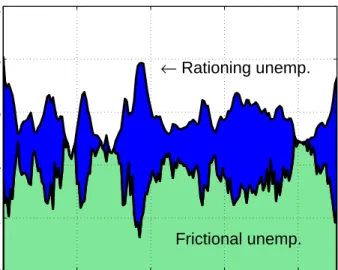
I decompose model-generated unemployment into historical time series for frictional and ra-tioning unemployment. This simulation uncovers quantitatively large cyclical fluctuations in fric-tional and rationing unemployment. In the model, as long as total unemployment is below 4.8 percent, it can all be attributed to matching frictions. On average, total unemployment amounts to 5.8 percent of the labor force, frictional unemployment to 3.6 percent, and rationing unemployment to 2.2 percent. But in deep recessions, when total unemployment reaches 8.0 percent, rationing unemployment increases above 6.0 percent, while frictional unemployment decreases below 2.0 percent.
The paper is organized as follows. Section2 presents the general model on which my analy-sis rests. Section3frames several influential search-and-matching models as special cases of the general model to show that they do not have job rationing. Section4theoretically studies unem-ployment and its components in a specific model in which job rationing arises from wage rigidity and diminishing marginal returns to labor. Section 5 calibrates this specific model to quantify fluctuations in rationing and frictional unemployment. Section6discusses normative implications and relates this work to the macroeconomic literature on unemployment. All proofs are in the Appendix.
2
General Model
This is a discrete-time model. Fluctuations are driven by technology, which follows a Markov process{at}+t=∞0.3
3This model takes the view that recessions are driven by aggregate-activity shocks and not by reallocation shocks, in line with empirical evidence (Abraham and Katz 1986;Blanchard and Diamond 1989;Hall 2005b). Thus I assume a stable matching function and, following the literature, I introduce aggregate technology shocks.
2.1
Household
The representative household is composed of a mass 1 of infinitely-lived workers. It has risk-neutral von Neumann-Morgenstern preferences over consumption, and it discounts future payoffs by a factor δ∈(0,1). It consumes all its income each period: Ct =Wt·Nt+πt, where Ct is consumption, Wt is the average real wage, andπt is the aggregate real profit of firms, which are owned by the household.4
2.2
Labor market
A continuum of firms indexed by i∈[0,1]hire workers. At the end of period t−1, a fraction s of the Nt−1 existing worker-job matches are exogenously destroyed. Workers who lose their job can apply for a new job immediately. At the beginning of period t, Ut−1 unemployed workers are looking for a job:
Ut−1=1−(1−s)·Nt−1. (1)
At the beginning of period t, firms open Vt vacancies to recruit unemployed workers. The number of matches made in period t is given by a constant-returns matching function h(Ut−1,Vt), differ-entiable and increasing in both arguments. Conditions on the labor market are summarized by the labor market tightnessθt≡Vt/Ut−1. An unemployed worker finds a job with probability f(θt)≡
h(Ut−1,Vt)/Ut−1 =h(1,θt), and a vacancy is filled with probability q(θt)≡ h(Ut−1,Vt)/Vt =
h(1/θt,1) = f(θt)/θt. In a tight market it is easy for jobseekers to find jobs—the job-finding probability f(θt)is high—and difficult for firms to hire workers—the job-filling probability q(θt) is low. Keeping a vacancy open has a per-period cost of c·at units of consumption. The recruit-ing cost c∈(0,+∞) captures the resources that firms must spend to recruit workers because of matching frictions. I assume no randomness at the firm level: a firm fills a job with certainty by opening 1/q(θt)vacancies. Thus, a firm spends c·at/q(θt)to fill a job. When the labor market is tighter, a vacancy is less likely to be filled, a firm must post more vacancies to fill a vacant job, and
4There is no labor-supply decision (neither number of hours nor labor market participation). This setup is standard in the literature. It is motivated by empirical work on the cyclical behavior of the labor market that suggests that hours per worker and labor force participation are quite acyclical (Shimer 2010).
recruiting is more costly.
Firm i decides the number Ht(i)≥ 0 of workers to hire at the beginning of period t. The aggregate number of recruits is Ht =R01Ht(i)di. Number of hires Ht, labor market tightnessθt, and unemployment Ut−1are related by the job-finding probability:
f(θt) =
Ht
Ut−1
. (2)
Upon hiring, Nt(i) = (1−s)·Nt−1(i)+Ht(i)workers are employed in firm i. The aggregate number of employed workers is Nt =
R1
0 Nt(i)di. When the labor market is in steady state, labor market tightness θ is related to employment N by an upward-sloping Beveridge curve that captures the equality of flows into and out of unemployment:
N= 1
(1−s) +s/f(θ). (3)
2.3
Wage schedule
The wage is set once a worker and a firm have matched. The marginal product of labor always exceeds the flow value of unemployment, which is normalized to zero, so there are always mutual gains from matching. There is no compelling theory of wage determination in such an environment (Hall 2005a; Shimer 2005). Hence, I consider in the next sections a broad set of wage-setting mechanisms: generalized Nash bargaining; Stole and Zwiebel (1996) intra-firm bargaining; and various reduced-form rigid wages. For now, I use a general wage schedule, which does not result from a specific wage-setting mechanism but nests as special cases the schedules studied later:
Wt(i) =W(Nt(i),θt,Nt,at), (4) where Wt(i) is the wage paid by firm i to all its workers at time t. W(.) is continuous and dif-ferentiable in all arguments. This schedule has a natural interpretation. Since technology at and employment Nt(i)determine current marginal productivity in the firm, they affect wages paid to
workers. Labor market tightness in the current periodθt determines outside opportunities of firms and workers, and also affects wages. Finally in a symmetric environment, because of the Markov property of the stochastic process for technology, aggregate employment Nt and technology fully determine the state of the economy and summarize the information set at time t; thus, conditional expectations as of time t are measurable with respect to (Nt,at). In so far as expectations about future economic outcomes affect wages, Nt and at affect wages.
2.4
Firms
Firms produce a homogeneous good sold on a perfectly competitive market. Firms take prices as given and I can normalize the price of the good to 1 in each period. A firm’s expected sum of discounted real profits is
E0 " +∞
∑
t=0 δt·π t(i) # , (5)whereπt(i)is the real profit of firm i in period t:
πt(i) =F(Nt(i),at)−Wt(i)·Nt(i)−
c·at
q(θt)
·Ht(i).
The production function F(·,·)is differentiable and increasing in both arguments. The aggregate real profit isπt =
R1
0 πt(i)di. The firm faces a constraint on the number of workers employed each period:
Nt(i)≤(1−s)·Nt−1(i) +Ht(i). (6) DEFINITION 1 (Firm problem). Taking as given the wage schedule (4), as well as labor mar-ket tightness, aggregate employment, and technology {θt,Nt,at}+t=∞0, the firm chooses stochastic processes {Ht(i),Nt(i)}+t=∞0 to maximize (5) subject to the sequence of recruitment constraints (6). The time t element of a firm’s choice must be measurable with respect to (at,N−1) where at≡(a0,a1, . . .,at).
I assume that the firm maximization problem is concave for any recruiting cost c∈(0,+∞). The unique solution to the firm problem is characterized by two equations. First, employment Nt(i)and
number of hires Ht(i)are related by
Ht(i) =Nt(i)−(1−s)·Nt−1(i)
because endogenous layoffs never occur in equilibrium. Second, employment Nt(i)is determined by the following first-order condition, which holds with equality if Nt(i)<1:
∂F ∂N(Nt(i),at)≥Wt(i) + c·at q(θt) +Nt(i) ∂W ∂N(Nt(i),θt,Nt,at)−δ(1−s)Et c·at+1 q(θt+1) (7)
This Euler equation implies that firm i hires labor until marginal revenue from hiring equals marginal cost. The marginal revenue is the marginal product of labor∂F/∂N. The marginal cost is
the sum of the wage Wt(i), the cost of hiring a worker c·at/q(θt), the change in the wage bill from increasing employment marginally Nt(i)·∂W/∂N, minus the discounted cost of hiring next period
δ·(1−s)·Et[c·at+1/q(θt+1)].
2.5
Equilibrium
DEFINITION 2 (Symmetric equilibrium). Given initial employment N−1and a stochastic process {at}+t=∞0for technology, a symmetric equilibrium is a collection of stochastic processes
{Ct,Yt,Nt,Ht,θt,Ut,Wt}+t=∞0
that solve the household and firm problems, satisfy the law of motion for unemployment (1), the law of motion for labor market tightness (2), the wage schedule (4), and the resource constraint in the economy, which imposes that all production is either consumed or allocated to recruiting:
Yt ≡ Z 1 0 F(Nt(i),at)di=Ct+ c·at q(θt) ·Ht.
Moreover, the wage {Wt}+t=∞0 satisfies the condition that no worker-employer pair has an unex-ploited opportunity for mutual improvement. The wage should neither interfere with the formation
of an employment match that generates a positive bilateral surplus, nor cause the destruction of such a match .
The equilibrium definition imposes that neither workers nor firms decide to break existing matches since any match generates some surplus.5 Since workers would never quit, the definition restricts wages to remain low enough in response to adverse technology shocks to avoid ineffi-cient separations. As inHall (2005a), the equilibrium of the model avoids the criticism directed at sticky-wage models byBarro (1977) because it satisfies the criterion that no employer-worker pair forgoes opportunities for bilateral improvement. In Sections3and4, I characterize and ana-lyze equilibria for various specifications of the production function and the wage schedule. I aim to determine whether jobs are rationed in these equilibria. But before proceeding, I define job rationing.
2.6
Job rationing
Consider a counterfactual environment in which matching frictions are absent. The matching pro-cess remains the same: firms open vacancies; firms and workers match; and the worker-firm pair either settles on a wage or dissolves the match. The matching technology characterized by the matching function h(U,V)remains the same. However, firms do not need to devote any resources (time or material) to recruiting because there are no matching frictions: the recruiting cost c con-verges to 0. When jobs are rationed, some unemployment remains in equilibrium. In other words, the economy does not converge to full employment even in the absence of matching frictions.
My study of job rationing focuses on static environments without aggregate shocks (at=a for all t ≥0) and with a labor market in steady state (equation (3) holds). This approach has three major advantages. First, I can analytically study the equilibrium and perform comparative statics to understand comovements of technology and labor market variables.6 Second, I can represent the equilibrium diagrammatically to provide an intuitive understanding of the mechanics of the model.
5The only separations observed in equilibrium are periodic, exogenous destructions of a fraction s of all jobs. 6The comparative-static approach is commonly used to understand theoretical properties of search models of the labor market (Hagedorn and Manovskii 2008;Mortensen and Nagyp´al 2007;Shimer 2005).
Third, the static model delivers the same qualitative predictions as a fully dynamic model.7
3
The Absence of Job Rationing in Existing
Search-and-Matching Models
I specialize the model presented in Section 2 to three influential search-and-matching models: the canonical search-and-matching model, its variant with diminishing marginal returns to labor in production, and its variant with rigid wages. I demonstrate that job rationing is absent from these models: the economy converges to full employment when recruiting cost c converge to 0. Hence, existing models consider that matching frictions are the sole source of unemployment and that eliminating frictions would eliminate unemployment. This underlying assumption strongly influences the welfare implications and policy recommendations derived from these models.
3.1
Mortensen-Pissarides model (MP model)
ASSUMPTION 1 (Constant returns to labor). F(N,a) =a·N.
ASSUMPTION 2. There existsβ∈(0,1)such that
W(Nt(i),θt,Nt,at) = c·β 1−β· at q(θt) +δ·(1−s)·Et at+1· θt+1− 1 q(θt+1) .
The MP model, characterized by Assumptions1and2, retains the key elements of the canonical search-and-matching model studied inPissarides(2000) andShimer(2005). Lemma1shows that the wage schedule specified by Assumption 2 corresponds to the generalized Nash bargaining
7In some of the specifications presented below, labor market tightness in the stochastic environment is invariant to technology, and solves the same equation as labor market tightness in any static environment. In other specifications, the equilibrium of the static model approximates the equilibrium of the fully dynamic model well, with the same qualitative properties. This approximation is valid for two reasons: (i) the labor market rapidly converges to an equilibrium in which inflows to and outflows from employment are balanced because rates of job destruction and job creation are large (Hall 2005a;Pissarides 2009;Rotemberg 2008); at the same time (ii) the recruiting behavior of firms is scarcely altered when they expect future shocks because technology is quite autocorrelated and shocks are of small amplitude.
solution, which allocates a fractionβ∈(0,1)of the surplus of a match to the worker, and the rest to the firm.
LEMMA 1 (Equivalence with Nash bargaining). Let W(·)be specified in Assumption2. Assume that Wt(i) in any period t in any firm i is determined by generalized Nash bargaining, and β is
workers’ bargaining power. Then Wt(i) =W(Nt(i),θt,Nt,at).
In the symmetric equilibrium of the MP model, the Euler equation (7) becomes
(1−β)·at= c·at q(θt) +c·δ·(1−s)·Et at+1· β·θt+1− 1 q(θt+1) .
I assume that technology follows a martingale: for all t ≥0, Et[at+1] =at. Then equilibrium labor market tightness is invariant to technology shocks, because the marginal recruiting costs, the wage, and the marginal product of labor increase in the same proportion as technology. Hence, θ is constant and determined by8
(1−β) =c· 1−δ·(1−s) q(θ) +δ·(1−s)·β·θ . (8)
Equation (8) also characterizes equilibrium labor market tightness in a static environment for any technology level a. Since labor market tightness is identical in any static or stochastic environment, I focus on a static environment. Equations (3) and (8) uniquely define equilibrium employment and labor market tightness as implicit functions N(c)andθ(c)of recruiting cost c. Proposition1shows that jobs are not rationed in the MP model because the economy converges to full employment when matching frictions vanish.
PROPOSITION 1 (Full employment in MP model). Under Assumptions1 and2, for any tech-nology a∈(0,+∞), limc→0θ(c) = +∞and limc→0N(c) =1.
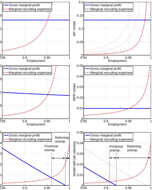
A simple diagram in Figure 1 explains this result. Expressing labor market tightness θ as a function of employment N, I represent equilibrium condition (8) on a plane with employment
8Even though the setup is slightly different, the equilibrium condition is similar to that derived inPissarides(2000) for the canonical model when the flow value of unemployment is zero.
on the x-axis. The horizontal line is the marginal profit from hiring labor gross of recruiting expenses, on the left-hand side of (8).9 By construction, gross marginal profit is independent of labor market tightnessθand recruiting cost c. Here, the gross marginal profit is simply the marginal product of labor. The upward-sloping line is marginal recruiting expenses, on the right-hand side of (8). These expenses are imposed by the presence of a positive recruiting cost c, directly through the opening of vacancies, and indirectly through wage bargaining. The intersection of these two curves determines equilibrium unemployment. As illustrated in Figure1, when the recruiting cost decreases, the marginal-recruiting-expense curve shifts down while the gross-marginal-profit curve is unchanged. Hence equilibrium employment increases. When recruiting cost c converges to 0, employment N converges to 1: there is full employment.
This result can also be interpreted from the perspective of bilateral bargaining theory. Broadly speaking, the difference between the marginal product of labor and the flow value of unemployment is proportional to the bilateral surplus from a match. Hence the surplus is positive and independent from aggregate employment. Once recruiting expenses are sunk, any match generates the same positive surplus that is shared between firm and worker by Nash bargaining over wages. When recruiting cost c converges to 0, recruiting a worker is costless; thus, the net profit from any new match is positive and firms open vacancies to create jobs until all workers are employed.
3.2
Large-firm model with Stole-Zwiebel intra-firm bargaining (SZ Model)
ASSUMPTION 3 (Diminishing marginal returns to labor). F(N,a) =a·Nα,α∈[0,1). ASSUMPTION 4. There existsβ∈(0,1)such that
W(Nt(i),θt,Nt,at) =
α·β
1−β·(1−α)·at·Nt(i)
α−1+c·(1−s)·δ·β·E
t[at+1·θt+1].
The SZ model, characterized by Assumptions3and4, retains the key elements of the large-firm search-and-matching models with diminishing marginal returns to labor and theStole and Zwiebel
9Both sides of the equation have been normalized by a/(1−β). In the next sections, I normalize other equilibrium conditions by technology a.
(1996) intra-firm bargaining procedure studied inCahuc et al.(2008) andElsby and Michaels(2008). The main departure from the MP model is introducing diminishing marginal returns to labor, which requires the bargaining procedure to be adapted. Lemma2shows that the wage schedule specified by Assumption4corresponds to theStole and Zwiebel(1996) bargaining solution, which allocates a fractionβ∈(0,1)of the marginal surplus to workers, and the rest to the firm.
LEMMA 2 (Equivalence withStole and Zwiebel(1996) bargaining). Let W(·)be specified in As-sumption4. Assume that the wage Wt(i)in any period t in any firm i is determined byStole and Zwiebel
(1996) bargaining, andβis workers’ bargaining power. Then Wt(i) =W(Nt(i),θt,Nt,at). In the symmetric equilibrium of the SZ model, the Euler equation (7) becomes
1−β 1−β·(1−α) at·α·Ntα−1= c·at q(θt) +c·δ·(1−s)·Et at+1· β·θt+1− 1 q(θt+1) .
As in the MP model, if technology follows a martingale, equilibrium labor market tightness θ is invariant to technology shocks. It is related to equilibrium employment N through the same equation that links them in a static environment:10
1−β 1−β·(1−α) α·Nα−1=c· 1−δ·(1−s) q(θ) +δ·(1−s)·β·θ (9)
Equations (3) and (9) implicitly define equilibrium employment and labor market tightness in any static environment as functions N(c)and θ(c)of recruiting cost c. Proposition 2shows that despite diminishing returns, jobs are not rationed in the SZ model as the economy converges to full employment when matching frictions disappear.
PROPOSITION 2 (Full employment in SZ model). Under Assumptions3and4, for any technol-ogy a∈(0,+∞), limc→0θ(c) = +∞and limc→0N(c) =1.
A diagram in Figure1represents equilibrium condition (9). The downward-sloping line is the marginal profit from hiring labor gross of recruiting expenses, on the left-hand side of (9). Here,
10Whenα=1, equilibrium condition (9) is the same as equilibrium condition (8) in the MP model. This is because the Nash bargaining solution and theStole and Zwiebel(1996) bargaining solution are identical when the production function exhibits constant marginal returns to labor.
the gross marginal profit is the marginal product of labor, minus the component of the wage inde-pendent of labor market tightnessθand recruiting cost c, minus the marginal change in the wage bill implied by the renegotiation of the wage between the firm and all the workers. The upward-sloping line is marginal recruiting expenses, on the right-hand side of (9). The sole difference from the MP model is that the gross marginal profit is downward sloping, because of diminishing marginal returns to labor. Jobs, however, are not rationed either in the SZ model: when recruit-ing cost c decreases to 0, the marginal-recruitrecruit-ing-expense curve shifts down; the gross-marginal-profit curve is independent of c and positive despite sloping down—it intercepts the N =1 line atα·(1−β)/[1−β·(1−α)]>0; therefore, the economy converges to full employment when c decreases to 0.
From the perspective of bilateral bargaining, the surplus from a marginal match always remains positive even though it decreases with aggregate employment because of diminishing marginal returns. When a marginal worker is recruited, intra-firm bargaining allocates a positive share of the marginal surplus to the firm, and reduces the wage paid to all workers in the firm. Accordingly, once recruiting expenses are sunk, the marginal profit from any new match created is positive. When the recruiting cost is zero, any match generates a positive net profit, and employers expand employment until all the labor force is employed. In spite of diminishing marginal returns to labor, jobs are not rationed because wages fall sufficiently when an increase in employment reduces the marginal product of labor.
3.3
Mortensen-Pissarides model with Rigid real wages (MPR Model)
I assume constant marginal returns to labor (Assumption1) and introduce theBlanchard and Gal´ı
(2010) wage schedule, which only partially adjusts to technology shocks.
ASSUMPTION 5 (Wage rigidity). There existsγ∈[0,1)and w0∈(0,+∞)such that
W(Nt(i),θt,Nt,at) =w0·aγt.
search-and-matching models with rigid real wages studied inShimer(2004),Hall(2005a), andBlanchard and Gal´ı
(2010). The main departure from the MP model is the introduction of wage rigidity. Nonetheless, if technology is bounded: a∈[a,a], the rigid wage schedule satisfies the equilibrium requirement that no inefficient separations occur if w0≤a1−γ(Hall 2005a). Since wages are rigid (γ<1), they are not proportional to technology and the invariance property of the MP and SZ models does not hold: labor market tightness fluctuates in this model.
In a static environment, the Euler equation (7) becomes11
1−w0·aγ−1=c·
1−δ·(1−s)
q(θ) . (10)
Equations (3) and (10) implicitly define equilibrium employment and labor market tightness as functions N(a,c) andθ(a,c) of technology a and recruiting cost c. Proposition3 shows that in spite of wage rigidity, jobs are not rationed in the MPR model.
PROPOSITION 3 (Full employment in MPR model). Under Assumptions1and5, for any a such that a≥w01/(1−γ), limc→0θ(a,c) = +∞ and limc→0N(a,c) =1. If a≤w
1/(1−γ)
0 , for any c>0,
θ(a,c) =0 and N(a,c) =0.
A diagram in Figure 1represents equilibrium condition (10). The horizontal line is marginal profit gross of recruiting expenses, which is marginal product of labor minus wage, on the left-hand side of (10). The upward-sloping line is marginal recruiting expenses, on the right-hand side of (10). The difference with the MP model is that gross marginal profit fluctuates when tech-nology changes, because of wage rigidity. Jobs, however, are not rationed in the MPR model ei-ther: when recruiting cost c decreases to 0, the marginal-recruiting-expense curve shifts down; the gross-marginal-profit curve is independent of c and positive for any technology level a≥w10/(1−γ); therefore, the economy converges to full employment when c decreases to 0.
11Letθ∗solve (8). If technology follows a martingale, equilibrium condition (8) in the MP model makes the same prediction as equilibrium condition (10) forγ=1 and
w0= c·β 1−β· 1 q(θ∗)+δ·(1−s)· θ∗− 1 q(θ∗) .
A constant wage is not the outcome of any bargaining, so it could allocate a negative share of the bilateral surplus from a match to the firm or the worker. Since I assume constant marginal returns to labor, the surplus of any match is proportional to the difference between the level of technology and the flow value of being unemployed, and it is independent of aggregate employment. For the equilibrium condition of private efficiency to be respected, the wage must be below the level of technology; otherwise any match that generates a positive surplus would be dissolved inefficiently. As a consequence, any match generates the same positive profit once recruiting expenses are sunk. Without recruiting expenses, the net profit from any match is positive and jobs are created until all the labor force is employed. If the wage is low enough for one match to be profitable, infinitely many jobs would be profitable without recruiting expenses and the economy would operate at full employment in spite of wage rigidity.
4
Cyclicality of Frictional and Rationing Unemployment
In existing models, there would not be any unemployment without matching frictions. By con-struction, matching frictions are the sole source of unemployment. This section presents a model in which unemployment may result from both matching frictions and job rationing. I present one possible source of rationing: the combination of some real wage rigidity with diminishing marginal returns to labor. I study theoretically how the interaction of these two sources generates cyclical fluctuations in unemployment.
4.1
Two assumptions
I assume diminishing marginal returns to labor in production (Assumption3) and real wage rigid-ity (Assumption5).12 The introduction of wage rigidity into the model follows the reduced-form approach of the literature.13 The simple wage schedule in Assumption5 could be interpreted as
12As shown in Section3, the assumptions have been introduced separately in existing models, but have never been combined.
13Most macroeconomic models in the search literature use reduced-form approaches to wage rigidity: Shimer (2004),Hall(2005a), andBlanchard and Gal´ı(2010) assume simple rigid-wage schedules;Gertler and Trigari(2009)
the outcome of complex wage-setting processes normally occurring in firms. Historic and ethno-graphic evidence presented below suggests that the schedule captures critical elements of the be-havior of wages. As inHall(2005a), it is possible to sustain an equilibrium in which wages never result in an allocation of labor that is inefficient from the joint perspective of the worker-firm pair, even though wages are not completely flexible. For instance, Lemma3states that under Assump-tion6, inefficient worker-firm separations can be avoided with high probability if wages are flexible enough.
ASSUMPTION 6. log(at+1) =log(at) +zt with zt ∼N(0,σ2)andσ∈(0,+∞).
LEMMA 3. Under Assumptions3,5, and6, a sufficient condition onγsuch that inefficient sepa-rations occur with a probability below p is
γ≥1−(1−α)· log(1−s)
σ·Φ−1(p),
where Φ is the cumulative distribution function of N(0,1). Under this condition, there are no inefficient separations when the technology shock zt satisfiesΦ(zt)≥p.
Under a technical assumption on the stochastic process followed by technology, Lemma3shows that some rigidity can be accommodated in equilibrium in a stochastic environment, as inefficient separations are guaranteed to be avoided as long as the amplitude of negative technology shocks is not too large.14 Importantly, this condition is independent from recruiting costs. It is therefore also valid in an environment without matching frictions. The condition is less stringent when the separation rate s is higher because exogenous separations reduce employment in firms at the be-ginning of each period, which increases the marginal product of labor through diminishing returns. For a given wage, a higher marginal product makes inefficient separations less likely. Through the same mechanism, both lower production-function parameterαand lower standard deviation of technology shocksσreduce the lower bound on the elasticityγdescribed in Lemma3.
assume that wages can only be renegotiated at distant time intervals.
14I chose Assumption6 for its simplicity and its empirical relevance. Similar results can be derived with more complex assumptions on the stochastic process followed by technology.
4.2
Existence of job rationing
I concentrate on a static environment.15 Equation (7) simplifies to
α·Nα−1−w0·aγ−1= [1−(1−s)·δ]· c
q(θ). (11)
Equations (3) and (11) uniquely define equilibrium employment and labor market tightness as implicit functions N(a,c)andθ(a,c)of technology and recruiting cost.
PROPOSITION 4 (Existence of job rationing). Under Assumptions3and5, for any technology a∈(0,aR)with
aR=w0 α
1−1γ ,
there exists a unique NR(a)∈(0,1)such that limc→0N(a,c) =NR(a). NR(a)solves
α·Nα−1−w0·aγ−1=0, (12)
and is therefore given by
NR(a) =
α
w0 1−1α
·a11−−αγ. (13)
With technology a∈(0,aR), equation (12) admits a unique solution NR(a)<1. NR(a)is equi-librium employment in an environment without matching frictions for, in the absence of frictions,
c=0 and equilibrium condition (11) becomes equation (12). Proposition4states that jobs are ra-tioned when technology is low enough, because the economy remains below full employment even when matching frictions disappear. The mechanism leading to job rationing is simple. The wage agreed upon by firms and job applicants does not fall as much as the marginal product of labor when technology declines, because of wage rigidity. Thus, the wage may be above the marginal product of the last workers in the labor force, because of diminishing marginal returns to labor. In that case, irrespective of matching frictions, not all workers can be profitably hired.
15In the Appendix, I compare the unemployment and labor market tightness series obtained when I solve this model exactly, and when I solve it in a series of static environment. While the time series obtained with these two numerical solution methods are quantitatively different, they are qualitatively very similar.
Even without matching frictions, the labor market may not clear because there is no mechanism to bring wages down to the market-clearing level. Firms meet job applicants sequentially, one at a time. The timing of meetings prevents firms from auctioning off jobs as in a perfectly competitive setting. Yet, the wage is privately efficient because it is below the marginal productivity of any worker paired with a firm, so the firm makes a non-negative profit by paying the wage and pursuing the match.
To measure the shortage of jobs on the labor market, independent of matching frictions, I define rationing unemployment URas UR(a)≡1−NR(a) =1− α w0 1−1α ·a11−−αγ. (14)
Matching frictions impose positive recruiting expenses on firms, which contribute to the marginal cost of labor, and lead firms to curtail employment. To measure unemployment attributable to positive recruiting costs, I define frictional unemployment UF as
UF(a,c)≡U(a,c)−UR(a). (15)
A diagram in Figure 1 represents equilibrium condition (11). The downward-sloping line is gross marginal profit, on the left-hand side of (11). Here, gross marginal profit is marginal prod-uct of labor minus the wage. The upward-sloping line is marginal recruiting expenses, on the right-hand side of (11). Rationing unemployment is unemployment prevailing when the recruit-ing cost c converges to zero. It is obtained at the intersection of the gross-marginal-profit curve with the x-axis because the marginal-recruiting-expense curve shifts down to the x-axis when c falls to 0. Total unemployment is obtained at the intersection of the gross-marginal-profit and marginal-recruiting-expense curves, and frictional unemployment is the difference between total and rationing unemployment. The diminishing-return and wage-rigidity assumptions (Assump-tions 3 and 5 ) are necessary for the existence of job rationing. Without the diminishing-return assumption , the gross-marginal-profit curve would be flat and would never intersect the x-axis on (0,1), so rationing unemployment would always be nil. Without the wage-rigidity assumption, the
gross-marginal-profit curve would not shift. There would be no guarantee that it intersects the x-axis and rationing unemployment may never be positive. With rigid wages, the intersection occurs for low levels of technology.
This result can be interpreted from the perspective of bilateral bargaining. In the model with job rationing, there is a range of technology and employment in which the wage would be too high for firms to extract a positive share of the surplus from worker-firm matches. In fact, when technology is low enough and employment is high enough, the wage is above the marginal product of labor, and, even when recruiting expenses are sunk, firms would make a negative profit from a match. Unlike in the models of Section3, jobs are rationed when technology is low enough: even if recruiting cost was zero, workers could not all be profitably employed and some unemployment would remain.
4.3
Comparative statics
To understand how job rationing and matching frictions generate cyclical fluctuations in unemploy-ment, I study how technology, as well as total, rationing and frictional unemployments comove by performing comparative statics with respect to technology.
PROPOSITION 5 (Cyclicality of frictional and rationing unemployment). Under Assumptions3 and5, for any technology a∈(0,aR):∂U/∂a<0,∂UR/∂a<0, and∂UF/∂a>0.
Around any equilibrium at which jobs are rationed, we have the following comparative-static results: when technology decreases, total unemployment increases, rationing unemployment in-creases, but paradoxically, frictional unemployment decreases. This proposition uncovers a novel mechanism behind unemployment fluctuations. In expansions, when technology is high enough, matching frictions account for all unemployment. But when technology is low enough and falls further in recessions, the rationing of jobs becomes more acute, driving the rise in total unem-ployment. Simultaneously, the number of unemployed workers attributable to matching frictions falls.
curve shifts down because the marginal product of labor falls while rigid wages adjust downwards only partially. At the current employment level, gross marginal profit falls short of marginal re-cruiting expenses. Firms reduce hiring to increase gross marginal profit. Lower rere-cruiting efforts by firms reduce labor market tightness and recruiting expenses. The adjustment process continues until a new equilibrium with higher unemployment is reached, when gross marginal profit equals marginal recruiting expenses.
When technology decreases, the gross-marginal-profit curve shifts down and rationing unem-ployment is mechanically higher. Irrespective of matching frictions, the shortage of jobs is more acute, and there are more unemployed workers and fewer vacancies. Once frictions are taken into account, a firm posting a vacancy will receive many applications from the large pool of unem-ployed workers, and it will be able to fill its vacancy rapidly at low cost. From the employment level prevailing when c=0, a smaller reduction in employment suffices to bring the economy to equilibrium. Consequently, frictional unemployment diminishes.
4.4
Empirical evidence
There is ample evidence in favor of the two critical assumptions of diminishing returns and wage rigidity. The model aims to describe cyclical fluctuations, and production inputs do not adjust fully to changes in employment at business cycle frequency. Capital is especially slow to adjust. If capital and labor are the only production inputs and capital is assumed to be constant in the short run, the production function takes the form proposed in Assumption3 and exhibits diminishing marginal returns to labor. At longer horizon, the production function could exhibit diminishing marginal returns to labor if some production inputs such as land or managerial talent are in fixed supply.
Furthermore, ethnographic evidence supports the rigid wage schedule chosen in Assumption5. The schedule depends neither on the marginal product of labor nor on labor market conditions. The disconnect between wages and both marginal productivity and labor market conditions can be explained by the rise of the personnel management movement after World War I, which led to the widespread adoption of internal labor markets within firms (Jacoby 1984). Doeringer and Piore
0.850 0.9 0.95 1 0.05 0.1 0.15 0.2 Employment MP model
Gross marginal profit Marginal recruiting expenses
0.850 0.9 0.95 1 0.05 0.1 0.15 0.2 Employment MP model
Gross marginal profit Marginal recruiting expenses
0.850 0.9 0.95 1 0.05 0.1 0.15 0.2 Employment SZ model
Gross marginal profit Marginal recruiting expenses
0.850 0.9 0.95 1 0.01 0.02 0.03 0.04 0.05 Employment MPR model
Gross marginal profit Marginal recruiting expenses
0.850 0.9 0.95 1 0.01 0.02 0.03 0.04 0.05 Employment
Model with job rationing
Gross marginal profit
Marginal recruiting expenses Rationing unemp. Frictional unemp. 0.850 0.9 0.95 1 0.01 0.02 0.03 0.04 0.05 Employment
Model with job rationing
Gross marginal profit Marginal recruiting expenses
Frictional unemp.
Rationing unemp.
Figure 1: EQUILIBRIA IN VARIOUS SEARCH-AND-MATCHING MODELS
Notes: These diagrams describe equilibria in static environments in the MP, SZ, and MPR models, as well as in the
model with job rationing. The two diagrams for the MP model represent the equilibrium for a calibrated recruiting cost (left) and lower recruiting costs (right). The two diagrams for the model with job rationing represent the decomposition of unemployment into rationing and frictional unemployment for high technology (left) and lower technology (right). Diagrams are obtained by plotting equilibrium conditions (8) (for the MP model), (9) (for the SZ model), (10) (for the MPR model), and (11) (for the model with job rationing) for a continuum of employment levels. The model with job rationing is calibrated in Table1. Other models are calibrated in the Appendix.
(1971) document that in internal labor markets, motivated by concerns for equity within firms, wages are tied to job description and are insensitive to labor market and marginal productivity con-ditions. Furthermore, labor market institutions sometimes hamper downward wage adjustments in the face of slack labor markets. For instance,Temin(1990) andCole and Ohanian(2004) explain the persistence of high real wages during the Great Depression by the National Industry Recov-ery Act of 1933. More recently, unions vetoed nominal pay cuts during the Finnish depression of 1991-1993 despite rampant unemployment (Gorodnichenko et al. 2009). Lastly, managerial best practices across countries and industries oppose pay cuts even when the labor market is slack, be-cause managers believe pay cuts antagonize workers and reduce profitability (Agell and Lundborg 1995;Bewley 1999;Blinder and Choi 1990;Campbell and Kamlani 1997). Natural experiments studying workers’ reactions to pay cuts strongly support managers’ views (Krueger and Mas 2004;
Mas 2006).
5
Quantitative Analysis
The previous section presented evidence supporting the diminishing-return and wage-rigidity as-sumptions. In this section, I directly calibrate wage rigidity and diminishing marginal returns to be consistent with microdata on wage dynamics and aggregate data on the labor share. I move be-yond the comparative-static results by computing impulse response function in the fully dynamic model. I use theFair and Taylor (1983) algorithm to quantify comovements in technology, total unemployment, frictional unemployment, and rationing unemployment when the model is simu-lated with actual U.S. technology. A byproduct of the quantitative analysis is to verify that the calibrated model describes well the U.S. labor market.
5.1
Calibration
I calibrate all parameters at weekly frequency (a week is 1/4 of a month and 1/12 of a quarter). Table 1 summarizes calibrated parameters. I first estimate the stochastic process for technology in U.S. data. I construct log technology as a residual log(a) =log(Y)−α·log(N). Output Y
and employment N are seasonally-adjusted quarterly real output and employment in the nonfarm business sector constructed by the Bureau of Labor Statistics (BLS) Major Sector Productivity and Costs (MSPC) program. The sample period is 1964:Q1–2009:Q2. To isolate fluctuations at busi-ness cycle frequency , I followShimer(2005) and take the difference between log technology and a low frequency trend—a Hodrick-Prescott (HP) filter with smoothing parameter 105. I estimate detrended log technology as an AR(1) process: log(at+1) =ρ·log(at) +zt+1with zt+1∼N(0,σ2). With quarterly data, I obtain an autocorrelation of 0.897 and a conditional standard deviation of 0.0087, which yieldsρ=0.991 andσ=0.0026 at weekly frequency.
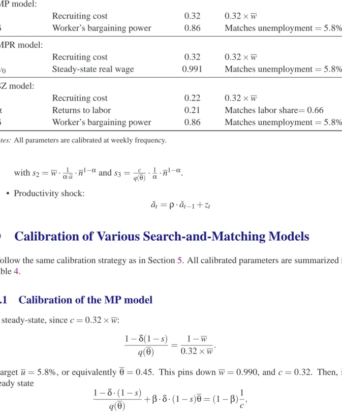
I now calibrate the labor market parameters: job destruction rate (s), recruiting cost (c), and matching function (ω,η). I estimate the job destruction rate from the seasonally-adjusted monthly series for total separations in all nonfarm industries constructed by the BLS from the Job Openings and Labor Turnover Survey (JOLTS) for the December 2000–June 2009 period.16 The average separation rate is 0.038, so s=0.0095 at weekly frequency. I estimate the recruiting cost from microdata gathered by Barron et al. (1997) and find that on average, the flow cost of opening a vacancy amounts to 0.098 of a worker’s wage.17 This number accounts only for the labor cost of recruiting. Silva and Toledo (2005) account for other recruiting expenses such as advertising costs, agency fees, and travel costs, to find that 0.42 of a worker’s monthly wage is spent on each hire. Unfortunately, they do not report recruiting times. Using the average monthly job-filling rate of 1.3 in JOLTS, 2000–2009, the flow cost of recruiting could be as high as 0.54 of a worker’s wage. I calibrate recruiting cost as 0.32 of a worker’s wage, the midpoint between the two previous
16December 2000–June 2009 is the longest period for which JOLTS is available. Comparable data are not available before this date.
17Using the 1980 Employment Opportunity Pilot Project survey (2,994 observations), they find that on average employers spend 5.7 hours per offer, make 1.02 offers per hired worker, and take 13.4 days to fill a position. Hence the flow cost of maintaining a vacancy open is 5.7/8×1.02/13.4≈0.054 of a worker’s wage. Adjusting for the possibility that hiring is done by supervisors who receive above-average wages as inSilva and Toledo(2005), the flow cost of keeping an open vacancy is 0.071 of a worker’s wage. With the 1982 Employment Opportunity survey (1,270 observations), the corresponding numbers are 10.4 hours, 1.08 offers, 17.2 days, and the flow cost is 0.106. With the 1993 survey conducted by the authors for the W. E. Upjohn Foundation for Employment Research (210 observations), the numbers are 18.8 hours, 1.16 offers, 30.3 days, and the flow cost is 0.117.
estimates.18 Next, I specify the matching function as
h(U,V) =ω·Uη·V1−η
with η=0.5, in line with empirical evidence (Petrongolo and Pissarides 2001). Last, I estimate matching efficiencyωwith seasonally-adjusted monthly series for number of hires, vacancy level, and unemployment level constructed by the BLS from JOLTS and the Current Population Survey (CPS) over the 2000–2009 period. For each month i, I calculate θi as the ratio of vacancies to unemployment and the job-finding probability fias the ratio of hires to unemployment. The least squares estimate ofω, which minimizes∑i(fi−ω·θ1i−η)2, is 0.93. At weekly frequency,ω=0.23. Next I calibrate the elasticityγof wages with respect to technology based on estimates obtained from panel data recording wages of individual workers. These microdata are more adequate be-cause they are less prone to composition effects than aggregate data. The survey of the literature by
Pissarides(2009) places the productivity-elasticity of wages of existing jobs in the 0.2–0.5 range in U.S. data.Pissarides(2009) argues, however, that models should be calibrated with the elasticity of wages of newly created jobs and not existing jobs. Estimating wage rigidity for newly created jobs is a arduous task. The standard approach is to measure wage rigidity among job movers. Unfor-tunately the composition of jobs accepted over the cycle fluctuates, biasing the analysis. Workers accept lower-paid, stop-gap jobs in recessions, and move to better jobs during expansions, biasing the estimated elasticity upwards. This composition effect is difficult to control for. A recent study byHaefke et al.(2008) estimates the elasticity of wages of job movers with respect to productivity using panel data for U.S. workers. They do not control for the cyclical composition of jobs; thus, their estimate is an upper bound on the elasticity of wages. For a sample of production and super-visory workers over the period 1984–2006, they obtain a productivity-elasticity of total earnings of 0.7. I setγ=0.7, a conservative estimate of wage rigidity.19
18Using the average unemployment rate and labor market tightness in JOLTS, I find that 0.89 percent of the total wage bill is spent on recruiting.
19This estimate of wage rigidity is conservative for two reasons: (i) 0.7 is an upward-biased estimate of the elas-ticity of wages; (2) 0.7 is an estimate of the elaselas-ticity of wages with respect to labor productivity Y/N, whereasγis the elasticity of wages with respect to technology a=Y/Nα. While technology and productivity are highly corre-lated, productivity is less volatile than technology and therefore an estimate of the elasticity of wages with respect to
Table 1: PARAMETER VALUES IN SIMULATIONS OF THE MODEL WITH JOB RATIONING
Interpretation Value Source
δ Discount factor 0.999 Corresponds to 5% annually
a Steady-state technology 1 Normalization
ρ Autocorrelation of technology 0.991 MSPC, 1964–2009
σ Standard deviation of shocks 0.0026 MSPC, 1964–2009
s Separation rate 0.0095 JOLTS, 2000–2009
ω Efficiency of matching 0.23 JOLTS, 2000–2009
η Unemployment-elasticity of matching 0.5 Petrongolo and Pissarides(2001)
γ Wage rigidity 0.70 Haefke et al.(2008)
c Recruiting cost 0.21 0.32×steady-state wage
α Returns to labor 0.67 Matches labor share=0.66
w0 Steady-state real wage 0.67 Matches unemployment=5.8%
Note: All parameters are calibrated at weekly frequency.
So far, I have estimated parameters from microdata or aggregate data, independently of the model. To conclude, I calibrate the steady-state wage w0 and the production function parameter
α such that the steady state of the model matches average unemployment u=5.8% and average labor share ls=0.66 in U.S. data. Average unemployment is computed from the seasonally-adjusted monthly unemployment rate constructed by the BLS from the CPS for the 1964–2009 period. These targets imply steady-state employment n =0.951 and steady-state labor market tightnessθ=0.45. In steady state a=1 and ls≡(w·n)/y=w0·n1−α. Therefore (11) becomes
ls=α−[1−δ(1−s)]· c
q(θ)·n 1−α,
which yieldsα=0.67 and w0=ls·nα−1=0.67.
Table 2: SUMMARY STATISTICS, QUARTERLY U.S. DATA, 1964–2009. U V θ W Y a Standard Deviation 0.168 0.185 0.344 0.021 0.029 0.019 Autocorrelation 0.914 0.932 0.923 0.950 0.892 0.871 Correlation 1 -0.886 -0.968 -0.239 -0.826 -0.478 – 1 0.974 0.191 0.785 0.453 – – 1 0.220 0.828 0.479 – – – 1 0.512 0.646 – – – – 1 0.831 – – – – – 1
Notes: All data are seasonally adjusted. The sample period is 1964:Q1–2009:Q2. Unemployment rate U is quarterly
average of monthly series constructed by the BLS from the CPS. Vacancy rate V is quarterly average of monthly series constructed by merging data constructed by the BLS from the JOLTS and data from the Conference Board, as detailed in the text. Labor market tightnessθis the ratio of vacancy to unemployment. Real wage W is quarterly, average hourly earning in the nonfarm business sector, constructed by the BLS CES program, and deflated by the quarterly average of monthly CPI for all urban households, constructed by BLS. Y is quarterly real output in the nonfarm business sector constructed by the BLS MSPC program. log(a)is computed as the residual log(Y)−α·log(N)where N is quarterly employment in the nonfarm business sector constructed by the BLS MSPC program. All variables are reported in log as deviations from an HP trend with smoothing parameter 105.
5.2
Simulated moments
I verify that the model provides a sensible description of reality by comparing important simulated moments to their empirical counterparts. I focus on second moments of the unemployment rate
U , the vacancy rate V , labor market tightnessθ=V/U , real wage W , output Y , and technology a.
Table2presents empirical moments in U.S. data for the 1964:Q1–2009:Q2 period. Unemployment rate, output, and technology are described above. The real wage is quarterly, average hourly earn-ing in the nonfarm business sector constructed by the BLS Current Employment Statistics (CES) program, and deflated by the quarterly average of monthly Consumer Price Index (CPI) for all urban households, constructed by BLS. To construct a vacancy series for the 1964–2009 period, I merge the vacancy data from JOLTS for 2001–2009, with the Conference Board help-wanted ad-vertising index for 1964–2001.20 I take the quarterly average of the monthly vacancy-level series,
20The Conference Board index measures the number of help-wanted advertisements in major newspapers. It is a standard proxy for vacancies (for example,Shimer 2005). The merger of both datasets is necessary because JOLTS
and divide it by employment to obtain a vacancy-rate series. I construct labor market tightness as the ratio of vacancy to unemployment. All variables are seasonally-adjusted, expressed in logs, and detrended with a HP filter of smoothing parameter 105.
Next, I log-linearize my model around steady state and perturb it with i.i.d. technology shocks
zt∼N(0,0.0026).21 I obtain weekly series of log-deviations for all the variables. I record values every 12 weeks for quarterly series (Y, W, a). I record values every 4 weeks and take quarterly
averages for monthly series (U, V, θ). I discard the first 100 weeks of simulation to remove the effect of initial conditions. I keep 100 samples of 182 quarters (2,184 weeks), corresponding to quarterly data from 1964:Q1 to 2009:Q2. Each sample provides estimates of the means of model-generated data. I compute standard deviations of estimated means across samples to assess the precision of model predictions. Table3presents the resulting simulated moments. Simulated and empirical moments for technology are similar because I calibrate the technology process to match the data. All other simulated moments are outcomes of the mechanics of the model.
The fit of the model is very good along several critical dimensions. First, the model amplifies technology shocks as much as observed in the data. In U.S. data, a 1-percent decrease in tech-nology increases unemployment by 4.2 percent and reduces vacancy by 4.3 percent. It therefore reduces labor market tightness, measured by the vacancy-unemployment ratio, by 8.6 percent.22 In the model, a 1-percent decrease in technology increases unemployment by 6.2 percent, reduces vacancy by 7.0 percent, and therefore reduces labor market tightness by 13.2 percent. Second, the response of wages to technology shocks in the model and the data are indistinguishable. In both cases, a 1-percent decrease in technology decreases wages by 0.7 percent. Third, simulated and empirical slopes of the Beveridge curve are almost identical. The slope, measured by the correlation of unemployment with vacancy, is -0.92 in the model and -0.89 in the data. Last, autocorrelations of all variables and behavior of output in the model match the data.
began only in December 2000 while the Conference Board data become less relevant after 2000, owing to the major role played by the Internet as a source of job advertising.
21The Appendix describes the log-linear model in details. 22The elasticity of unemployment with respect to technologyεU
a is the coefficient obtained in an OLS regression
of log unemployment on log technology. This coefficient can be derived from Table2:εU
a =ρ(U,a)×σ(U)/σ(a) =
−0.478×0.168/0.019=−4.2. All other elasticities are computed similarly. Sinceθ=V/U ,εθa=εV
Table 3: SIMULATED MOMENTS WITH TECHNOLOGY SHOCKS U V θ W Y a Standard Deviation 0.119 0.142 0.256 0.014 0.024 0.019 (0.021) (0.022) (0.044) (0.002) (0.004) (0.003) Autocorrelation 0.939 0.847 0.913 0.884 0.898 0.884 (0.020) (0.045) (0.028) (0.036) (0.032) (0.036) Correlation 1 -0.931 -0.979 -0.986 -0.991 -0.986 (0.020) (0.007) (0.004) (0.003) (0.004) – 1 0.986 0.935 0.929 0.935 (0.004) (0.019) (0.021) (0.019) – – 1 0.975 0.974 0.975 (0.008) (0.008) (0.008) – – – 1 0.999 1.000 (0.001) (0.000) – – – – 1 0.999 (0.000) – – – – – 1
Notes: Results from simulating the log-linearized model with stochastic technology. All variables are reported as
logarithmic deviations from steady state. Simulated standard errors (standard deviations across 100 simulations) are reported in parentheses.
However, the model does not perform well along one important dimension: the correlation of labor market variables and wages with technology. Simulated correlations of unemployment, va-cancy, and labor market tightness with technology are close to 1, but empirical correlations are below 0.5. Similarly, aggregate wages vary twice as much in the data as in the model. Demand shocks, financial disturbances, and nominal rigidities, absent from the model but empirically im-portant, could explain these discrepancies. The simplicity of the model prevents it from achieving the degree of volatility observed in the data: while amplification of technology shocks is as strong as in the data, simulated standard deviations of wage W and labor market variables U , V , andθare inferior to their empirical counterparts because some sources of volatility are omitted.
This simulation exercise contributes to a large literature on the role of wage rigidity in ex-plaining unemployment fluctuations. Following theShimer(2005) critique of the standard
search-and-matching model, several papers introduced wage rigidity to increase unemployment volatility (Gertler and Trigari 2009;Hall 2005a; Hall and Milgrom 2008). These papers were criticized for exaggerating the rigidity of wages in spite of empirical evidence suggesting that wages