The KOSPI200 Implied Volatility Index: Evidence of Regime Switches in Volatility Expectations *

The KOSPI200 Implied Volatility Index:

Evidence of Regime Switches in Volatility Expectations

Wakayama University, Wakayama, Japan

Moo-Sung Kim

Pusan National University, Busan, Korea

Kazuhiko Nishina

Osaka University, Osaka, Japan

Received 15 December 2006; Accepted 16 January 2007

Abstract

This study develops a new KOSPI200 implied volatility index and examines its infor-mational content and nonlinear dynamics. The construction of this new benchmark for volatility expectations follows the methodology for calculating the new VIX index from S&P500 options. The empirical evidence suggests that the expected level of volatility in the Korean stock market has been steadily falling since the inception of option trading and the onset of the Asian financial crisis. Implied volatility is found to reflect useful in-formation on future volatility that is not contained in the history of returns, even after allowing for leverage effects. Markov regime-switching models suggest that nonlinearities in volatility expectations are not likely to be driven solely by the asymmetric impact of news but also by regime-dependencies in the realignment mechanism adjusting for fore-cast errors. The adjustment process is likely to be significant during regimes of lower volatility expectations but financial crises seem to elevate the level of anticipated volatil-ity and impair its adaptive dynamics.

Keywords: KOSPI200 Implied volatility index; Markov regime-switching model;

Asym-metric effects; Stock market volatility; Nonlinear dynamics

* This study was supported by Grants-in-Aid for Scientific Research from the Japan Society for the Promotion of Science. This authors are also grateful to the anonymous referees and participants at the first International Conference on Asia Pacific Financial Markets held by the Korea Securities Association. Any remaining errors are our own.

** Corresponding Author. Address: Faculty of Economics, Wakayama University, Sakaedani 930, Wakayama 640-8510, Japan; E-mail: nebilmg@eco.wakayama-u.ac.jp;

1. Introduction

The increasing level of fluctuations in foreign exchange and asset prices, especially during financial crises, poses important questions as to what factors determine the reaction of speculative markets to the arrival of new information and ultimately, what constitutes excessive volatility. Under the assumption of informationally effi-cient markets, the behavior of security prices should be fully and correctly reflective of the aggregate content of economic information. This implies that the time-series of changes in asset prices can be regarded as a reconstruction of the flow of new infor-mation into financial markets. In addition to this classical approach in the analysis of market volatility based on historical data, it is equally important to focus on volatility expectations, which are essential in investment decisions-making, risk-hedging and market regulation. Indeed, expectations can exert significant influence on market prices and can even affect the course of monetary policy, especially during periods of

financial turmoil. But, the empirical tests of ex ante market volatility remain

im-peded by the fact that expected volatility is rather difficult to ascertain with much accuracy. Again, the recourse is usually made to the time-series of historical price changes that provide a source of information on which rational expectations based on all available information can be formed. But, the alternative estimates of market volatility implicit in options prices can provide forward-looking measures of expected volatility. Thus, an implied volatility index is not only consistent with rational expec-tations in the sense that is reflects all available information. This index has also the merit of aggregating volatility anticipations from the wide range of exercise prices and options maturities.

There is strong evidence in support of the usefulness of implied volatility for fore-casting purposes. The early study by Day and Lewis (1992) provides evidence of sig-nificant informational content but also of some degree of inefficiency in the sense that incremental information is still contained in conditional volatility based on the gen-eralized autoregressive conditional heterosckedasticity (GARCH) model. Though Canina and Figlewski (1993) also suggest the lack of correlation between the implied volatility from S&P100 index options and future volatility, the evidence from Jorion (1995) and Amin and Ng (1997), suggests that albeit biased, implied volatility is an efficient estimate of foreign exchange volatility. The empirical literature from more

recent studies including Prabhala (1998) who adjust for maturity mismatch problems, as well as Blair, Poon and Taylor (2003) Nishina, Maghrebi and Kim (2006) who ap-ply out-of-sample forecasting tests, offers stronger evidence that implied volatility is associated with better predictive accuracy than alternative forecasts based on the time-series of returns. The evidence from Becker, Clemens and White (2006) lends further support to the informational efficiency of S&P500 implied volatility.

There is also a growing interest by monetary policymakers in the estimates of im-plied volatility which provide useful information on consensus expectations and mar-ket beliefs. The reference to marmar-ket sentiment and implied functions from options prices in the monetary policy meetings of the Bank of England adds to the increasing realization that implied volatility is useful in assessing the level of uncertainty about future interest rates and economic variables. This interest is also justified in light of evidence that implied volatility indices are useful for Value-at-Risk analysis as shown by Giot (2005) and that they provide measures of market sentiment as suggested by Whaley (2000) and Simon (2003). Also, the new VIX index derived from S&P500 op-tions is shown by Carr and Wu (2006) to contain useful information on the level of uncertainty preceding policymakers’ decisions on the Federal Reserve Fund Rate. Earlier evidence from Neely (2005) suggests that changes in implied volatility de-rived from options prices on Eurodollar futures interest rates are reflective of signifi-cant news related to the equity market and the anticipation of shifts in monetary pol-icy, among others. There is also evidence from Fornari (2004) for instance, that the impact of macroeconomic information such as US economic indicators is reflected in the behavior of implied volatility from swaptions prices.

In light of this increasing literature on the usefulness of implied volatility, the pre-sent study develops a new KOSPI200 implied volatility index following the methodol-ogy used in the construction of the new VIX for S&P500 index by the Chicago Board of Options Exchange. Given the increasing integration of international financial markets and the steady growth in the trading volume of KOSPI200 options, the in-troduction of this new benchmark of volatility expectations for the Korean equity market should be viewed as a natural step in the development of Korean financial

derivatives. The new volatility index can also be useful in providing an ex ante

meas-ure of uncertainty, and provide the basis for international comparison with the exist-ing benchmarks of volatility expectations.

in providing, to the best knowledge of the authors, the first index of implied volatility for the Korean stock market. The present analysis is also aimed at examining the informational content of volatility expectations and their nonlinear dynamics. This analysis can hence, be useful in shedding light on the behavior of volatility anticipa-tions with respect to significant events including the onset of the Asian financial cri-sis, which coincided with the inception of trading in KOSPI200 options, and the in-formation technology bubble in 2000, inter alia. It also addresses important questions such as how implied volatility behaves in response to financial crises, whether it con-tains useful information judging from its relationship with realized volatility, whether its dynamics can be characterized by nonlinearities in terms of regime shifts, and to what extent an error-correction mechanism is embedded in these stochastic dynamics.

The remainder of the paper is structured as follows. The next section presents a brief review of the methodology underlying the computation of KOSPI200 implied volatility index and examines its distributional properties. Section 3 assesses the effi-ciency of this index in terms of the significance of its relationship with realized vola-tility. Section 4 examines the nonlinear dynamics of implied volatility using Markov regime-switching models. Section 5 concludes the paper.

2. Implied Volatility Index: Estimation and Distributional

Properties

The process of numerically deriving estimates of implied volatility from option premia can be fraught with difficulties stemming for instance from the failure of the iterative process to convergence. The numerical procedure, which is aimed at mini-mizing the difference between theoretical and market prices is often based on the Black-Scholes (1973) theoretical option pricing model or its Merton’s dividend-augmented version. The non-convergence problems may be due to the market mis-pricing of options and/or to the misspecification of the theoretical option mis-pricing model. It is difficult to reconcile Black-Scholes theoretical modelling and its underly-ing assumption of constant volatility with the strong empirical evidence of ‘volatility smiles’, which characterize the relationship between exercise prices and implied vola-tility. There are several studies that propose ‘model-free’ approaches, in an attempt to avoid misspecification problems. The literature includes for instance, the

method-ology by Britten-Jones and Neuberger (2000), which draws on the conventional pro-cedure of fitting interest rates to bond prices, as well as alternative approaches based on interpolation, polynomial smoothing or splines smoothing of the options pricing function.

Unlike the original VIX index based on the Black-Scholes implied volatility from S&P100 options, the methodology underlying the new VIX index constitutes a ‘model-free’ approach to the estimation of implied volatility. It approximates the variance of theoretical at-the-money options with thirty days remaining to expiration and with exercise price equal to the estimated forward index level. In the absence of a theoreti-cal option pricing model, this approximation process relies on the volatility structure recovered from the observed range of exercise prices and option maturities. The cal-culation methodology does not rely solely on near- or at-the-money options but

in-volves in-the-money options as well.1)

The model-free approach is hereafter briefly reviewed for the purposes of examin-ing particular measurement issues in the case of the new KOSPI200 implied volatil-ity index. The process is initiated with the selection of options with near-term and next-term maturities. In order to reduce measurement errors, the rollover process to the next maturity occurs when the time to expiration of near-term maturity options falls below eight days. On each trading date, the spreads between call and put option premiums with equal exercise prices are calculated and the at-the-money exercise price is subsequently identified in association with the minimum spread. This

at-the-money exercise price K• is allowed to differ across near-term and next-term

maturi-ties.

The forward index level r ( )

F=K•+eτ C−P is determined for each contract month

on the basis of the corresponding at-the-money exercise price and spread between call-put premiums. It is noted that the cost-of-carry modelling of this forward price,

with risk-free raterand time-to-expiration τ, is not based on the observed spot index

prices but on the at-the-money exercise prices. The subsequent determination of the

exercise price immediately below this forward index level K₀<F is straightforward.

Option prices are then ranked in the ascending order of exercise prices, and only

1) The procedure for calculating the new VIX index is discussed in further details with illustrative examples from online publications by the Chicago Board of Options Exchange. The study by Carr and Wu (2006) provide a comparative analysis of the old CBOE-VIX and new VIX index including a discussion of their methodological differences.

the-money put options K<K₀ and in-the-money call options K>K₀ are

subse-quently selected and their marginal contributions to implied volatility for each ma-turity are calculated.

The marginal contribution 2

( K Ki i )e Q Kr ( i) τ

Δ of each in-the-money option is

func-tion of its opfunc-tion premiumQas well as the spread between exercise prices.2) It is a

decreasing (increasing) function of the exercise price for call (put) options. The cumu-lative contributions result in the estimation of the implied variance as follows

( )

∑

For each trading date, an estimate of implied variance is obtained for each matur-ity. Because of differences in the time-to-expiration between these estimates, the ap-proximation of the annualized estimate of implied variance from the hypothetical op-tion with thirty-days to maturity requires the following interpolaop-tion process

2 1 2 1 2 1 30 30 2 2 2 365 1 1 2 2 30 N N N N N N N N N N τ τ τ τ τ τ σ =_⎜⎜⎛τ σ ⎡⎢ − ⎤⎥+τ σ ⎢⎡ − ⎤⎥⎞_⎟⎟× − − ⎢ ⎥ ⎢ ⎥ ⎣ ⎦ ⎣ ⎦ ⎝ ⎠ ,

where Nτis time until expiration expressed in minutes. Hence, it appears that the

methodology is effective in accounting for various features of option trading and mar-ket valuation through the selection of in-the-money options and near-term and next-term options. This approach is conducive towards the reduction of measurement er-rors, limitation of misspecification erer-rors, the focus on most liquid option quotes and the accounting for nonlinearities in the relationship between option premiums and exercise prices.

The new KOSPI200 implied volatility index is estimated as the square-root of the implied variance from options quotes at 3 pm obtained from the Korea Exchange. For comparative purposes, the time-series of the new VIX index for S&P500 index are obtained from Thomson Financial Datastream. The sample period extending from

2) The options strike interval is set at 5.00 points for options trading on the quarterly cycle and 2.50 for the remaining options. Since the focus is made on near-term and next-term maturities for the purposes of cal-culating the new KOSPI200 implied volatility, the spread between exercise prices is 2.50. The settlement date is function of the last trading day, which is determined as the second Thursday of the contract month.

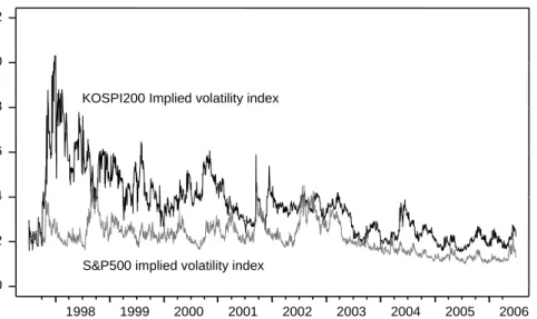
Figure 1. The behavior of KOSPI200 and S&P500 implied volatility indices 0.0 0.2 0.4 0.6 0.8 1.0 1.2 1998 1999 2000 2001 2002 2003 2004 2005 2006

KOSPI200 Implied volatility index

S&P500 implied volatility index

July 1997 through June 2006, spans a total of 109 near-term and next-term maturi-ties, extending to August 2006. The middle rate on the three-month Korean

Certifi-cates of Deposit rates is used as proxy for risk-free rates.3)

It appears from Figure 1, which describes the behavior of the new implied volatility index, that volatility expectations ebb and flow, with peaks seemingly related to sig-nificant economic events in the Korean and US markets. The new KOSPI200 implied volatility index tends to be higher than the new VIX index. This is particularly true with respect to the Asian financial crisis where volatility anticipations in the Korean market are reflective of the heightened level of uncertainty in regional stock markets. Despite the observed signs of responsiveness, volatility expectations in the Korean market appear to be less affected by other significant events such as the Russian debt and LTCM crises in 1998 or the Latin American debt crisis, which are more evident in the behavior of the new VIX series for the US market. In contrast, the burst of the information technology bubble is not apparently associated with a significant surge in volatility expectations.

3) The trading period of the European-style KOSPI200 index options extends from 9 am to 3.15 pm, except for the last trading day, on which options trading ends at 2.50 pm. Thus, the calculation of KOSPI200 im-plied volatility index with option quotes at 3 pm, which coincides with the end of trading in the spot mar-ket, serves also the purpose of avoiding the measurement problems associated with non-synchronous trad-ing.

Table 1. Distributional properties and stationarity tests

KOSPI200 index S&P500 index Implied volatility Stock returns Implied volatility Stock returns Mean - Total Period 0.3600 0.0003 0.2172 0.0001 - July 1997 ~ Dec. 2001 0.4519 0.0001 0.2477 0.0002 - Jan. 2002 ~ June 2006 0.2685 0.0006 0.1868 0.0001 Standard Deviation - Total Period 0.1478 0.0232 0.0678 0.0116 - July 1997 ~ Dec. 2001 0.1467 0.0288 0.0482 0.0127 - Jan. 2002 ~ June 2006 0.0731 0.0158 0.0709 0.0103 Skewness - Total Period 1.2201 0.0654 0.5632 -0.0531 - July 1997 ~ Dec. 2001 1.0379 0.1281 1.3567 -0.2210 - Jan. 2002 ~ June 2006 0.3770 -0.2480 1.2539 0.2537 Kurtosis - Total Period 5.1024 6.4604 3.2043 6.1259 - July 1997 ~ Dec. 2001 4.6881 5.0547 5.4599 5.8273 - Jan. 2002 ~ June 2006 1.7780 4.6576 3.9438 6.0067 Jarque-Bera - Total Period 1013.71 1171.15 128.06 955.44 - July 1997 ~ Dec. 2001 349.30 209.01 654.45 399.23 - Jan. 2002 ~ June 2006 100.86 146.43 351.21 454.81 ADF statistic - Total Period -6.549a* _-45.971c* _-5.023a* _-49.703c* - July 1997 ~ Dec. 2001 -4.734 a* _-32.071c* _-5.498b* _-34.378c* - Jan. 2002 ~ June 2006 -3.562a** _-33.869c* _-4.025a* _-36.298c* Notes) The sample period extends from July 7, 1997 to June 30, 2006. JB is the standard Jarque-Bera

nor-mality test distributed asχ2

on the null. The series of stock market returns and changes in implied volatility are calculated with log differences. ADF statistic denotes the Augmented Dickey-Fuller tests of stationarity, a with intercept and trend terms, b with intercept only, and c with none. Signifi-cance at 1%, and 5% levelis denoted by *, and ** respectively.

It is noted that the perceived level of uncertainty in the Korean equity market has been steadily falling since the Asian financial crisis. The stronger tendency for con-vergence in implied volatility over more recent periods, is consistent with evidence from Nishina et al. (2006) based on the behavior of the Nikkei225 implied volatility index relative to the new VIX index. This realignment in volatility expectations

across countries may be reflective of stronger integration among international stock markets.

As indicated by the distributional statistics reported in Table 1, volatility expecta-tions in the Korean market are typically higher than those in the US market. How-ever, with the total sample is divided into two equal sub-periods, it appears that the differences in volatility are more salient during the more volatile crisis period of early KOSPI200 option trading. Implied volatility in the Korean market is not only found to be higher than in the post-crisis 2001~2006 period, but it also exhibits more vola-tility of its own, judging from the sample estimates of standard deviations. The Asian financial crisis seems to exert a significant increase in the perceived level of uncer-tainty as well as the degree of fluctuations in volatility expectations. The estimates of implied volatility are on average, found to be close to the annualized standard devia-tions of returns. Indeed, the average expected volatility is reflective of the changing level of uncertainty from the early trading to post-crisis periods, which are associated with annualized standard deviations of 55% and 30%, respectively. The higher mo-ments suggest that the distributions of returns and implied volatility are leptokurtic and the Jarque-Bera statistics strongly reject the hypothesis of normal distribution. The results of unit-root tests indicate that the time-series of stock market returns and implied volatility are stationary for both markets.

3. The Relationship between Implied Volatility and Realized

Volatility

In order to assess the significance of the information contained in implied volatility, it is important to examine its long-term relationship with realized volatility. The ex post estimates of realized volatility are represented by the standard deviation

(

)

σ =

∑

30 calendar days. This period spans the life of the hypothetical option used in deriv-ing the new implied volatility index. The relative spread between the implied

volatil-ity index and the annualized realized volatilvolatil-ity ξ_t =(v_t −σ σ_t) / _t provides a

standard-ized measure of daily forecast errors. As exhibited in Figure 2, the behavior of fore-cast errors is suggestive of frequent shifts between periods of volatility overshooting

Figure 2. The relative spread between implied volatility and realized volatility -100 -50 0 50 100 150 -100 -50 0 50 100 1998 1999 2000 2001 2002 2003 2004 2005 2006

KOSPI200 implied volatility to r ealized v olatility spr ead ( % )

S&P500 implied volatility

to r ealized v olatility spr ead ( % )

and periods of volatility underestimation in the Korean market. There is stronger tendency for an upward bias with respect to the new VIX for the US market, which is consistent with evidence from S&P100 index options by Fleming (1998).

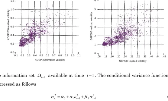
Judging from the sign and magnitude of errors in volatility expectations, the evi-dence suggests that because of its upward bias, implied volatility is not a perfect fore-cast of future volatility. However, the long-run relationship appears to be positive, as suggested by Figure 3, which plots realized volatility against implied volatility as well as by regression results, which are not reported here for the sake of brevity. The regression analysis of this long-term relationship with daily observations may suffer from errors-in-variables problems, which can be reflected by negative intercepts as noted by Christensen and Prabhala (1998), as well as from measurement errors from overlapping observations. Alternatively, the characterization of the efficiency of vola-tility expectations and assessment of its relationship with realized volavola-tility can be achieved by testing for its relative informational content with respect to forecasts based on GARCH modelling.

An important merit of GARCH modelling is that it can capture patterns of persis-tence and clustering in market volatility. The parsimonious GARCH (1,1) model, hereafter referred to as Model-A, can be described by the conditional mean equation

0

t t

Figure 3. The relationship between realized volatility and implied volatility index 0.0 0.2 0.4 0.6 0.8 1.0 1.2 0.1 0.2 0.3 0.4 0.5 0.6 0.7 0.8 0.9 1.0 1.1 KOSPI200 implied volatility

KO S P I200 r e a liz ed v o la ti lit y .0 .1 .2 .3 .4 .5 .6 .08 .12 .16 .20 .24 .28 .32 .36 .40 .44 .48 S&P500 implied volatility

S& P500 r eali z ed v o lat ili ty

the information set Ω_t−1 available at time t−1. The conditional variance function is

expressed as follows

2 2 2

0 1 1 1 1

t t t

σ =α +α ε₋ +β σ ₋ (1)

For the conditional variance to be well defined, all parameters should be non-negative. This is rather a sufficient but not necessary condition for non-negativity of the conditional variance. This model equation (1) imposes a symmetric response to volatility shocks irrespective of their sign. It is however important to test for the presence of asymmetries in the GARCH modelling of volatility because of the likeli-hood of distinct reactions of market volatility to negative shocks relative to good news. The leverage effects suggest that market volatility is likely to increase in bearish markets and decrease in bullish ones and that volatility rises more in response to negative than positive shocks. The model proposed by Glosten, Jagannathan and Runkle (1993) expresses the conditional variance as a function not only of the magni-tude of lagged residuals but of their sign as well.

2 2 2 2

0 1 1 1 1 1 1

t t t dt t

σ =α α ε+ − +β σ− +λ −ε− (2)

In this GJR-GARCH modelling of market volatility, drepresents the indicator

func-tion that associates the value of one to negative shocks (d_t−₁ =0 ifε_t−₁<0), and zero

otherwise. It is possible using Model-B described by equation (2) to test for the

In order to assess the informational content of volatility expectations, the condi-tional variance function is extended to include past observations of implied variance.

2 2 2 2

0 1 1 1 1 1 1

t t t vt

σ =α α ε+ − +β σ− +π − (3)

This modelling follows the approach proposed by Day and Lewis (1992), and Lamoureux and Lastrapes (1993) who test for the significance of the incremental in-formation embedded in options prices about future volatility, judging from the sign

and magnitude of π₁ parameters. As suggested by Amin and Ng (1997), Model-C

described by equation (3) can be further extended to include not only past implied variance but also contemporaneous volatility in order to account for any remaining significant information in the current levels of implied volatility. Model-D repre-sented by equation (4) expresses the conditional variance function as.

2 2 2 2 2

0 1 1 1 1 1 1 0

t t t vt vt

σ =α +α ε₋ +β σ₋ +π ₋ +π (4)

When the parameters π₀ and π₁= −π α β₀( + ) are found to be significant while

GARCH parameters are not, there is evidence of implied volatility containing all past and contemporaneous information about future volatility. A similar approach is also applied with respect to the GJR model of asymmetric response to news. Thus, in Model-E of equation (5), the conditional variance function includes past observations of implied variance while Model-F represented by equation (6) considers the impact of both past and current levels of implied variance.

2 2 2 2 2 0 1 1 1 1 1 1 1 1 t t t dt t vt σ =α +α ε₋ +β σ₋ +λ ₋ε₋ +π ₋ (5) 2 2 2 2 2 2 0 1 1 1 1 1 1 1 1 0 t t t dt t vt vt σ =α +α ε₋ +β σ₋ +λ ₋ε₋ +π ₋ +π (6)

The estimation results for the various specifications of the conditional variance us-ing the quasi-maximum likelihood method are reported in Table 2 and Table 3 for the Korean and US markets, respectively. Judging from the significance of both GARCH and residuals parameters in Model-A, there is evidence of volatility persistence form the estimation of the parsimonious GARCH models for both markets. The positive

and significantλcoefficients in the GJR Model-B are also indicative of the

Given the significance of π₁coefficient and the statistically insignificant GARCH and residuals parameters in Model-C, there is evidence that past observations of implied variance contain useful information about the volatility-generating process. This re-sult is suggestive of the informational efficiency of implied volatility and it is consis-tent with the empirical evidence from Harvey and Whaley (1992) and Lamoureux and Lastrapes (1993).

When past and current levels of implied variance are included in Model-D, the sig-nificance of all model parameters fades away for the Korean market. For the US

mar-ket however, the evidence of significant π parameters suggests that implied

volatil-ity contains useful incremental information. But given the significance of GARCH

Table 2. GARCH modelling of Korean market volatility and the informational content of implied variance

Model

Parameters Model-A Model-B Model-C Model-D Model-E Model-F 0 μ 0.0811b _{0.0424 0.0471 0.0833}b _{0.0444 0.0922}a 0 α 0.0019b _0.0017b _-0.0255c _{-0.0397 -0.0154}c _-0.0114c 1 α 0.0559a _0.0251b _{0.0290 0.0058 -0.0220 -0.0377}b 1 β 0.9429a _0.9507a _{0.0546 -0.0870 0.4991}a _0.6893a λ 0.0462a _0.1631a _0.1380a 1 π 0.0036a _{0.0017 0.0018}a _-0.0020 0 π 0.0026 0.0031b LB 0.119 0.129 0.299 0.214 0.244 0.204 LM 0.949 0.918 0.716 0.771 0.922 0.987 Log-L 5809.86 5817.42 5839.97 5850.40 5847.29 5861.65 Excess log-L 7.56 30.11 40.54 37.43 51.79

Notes) The sample period of daily observations extends from July 7, 1997 to June 30, 2006. Models A~F refer to the conditional variance functions defined by equations (1) to (6) respectively. For the pur-poses of clear presentation, the parameters estimates μ0and α0 are multiplied by 10

2

and 103, re-spectively. Significance at the 1, 5 and 10% level is denoted by a, b and c, respectively. LB refers to the p-values associated with Ljung-Box test for serial correlation in squared residuals up to the 10th order. LM refers to p-values of Lagrange-Multiplier test for remaining ARCH effects. Both tests are distributed asχ2

on the null. LogL is the estimated log-likelihood function. Excess log-L is the excess log-likelihood with respect to Model-A.

parameters, the information contained in implied volatility is not sufficient to fully explain the behavior of market volatility. Furthermore, the addition of lagged obser-vations of implied variance into the GJR Model-E whittles down the significance of GARCH parameters but not that of leverage effects. There remains evidence of the asymmetric impact of news even upon including both lagged and current levels of im-plied volatility in GJR Model-F. Judging from the improved log-likelihood function for both markets, this model is found to provide a better description of the stochastic be-havior of market volatility.

On aggregate, the evidence suggests that implied volatility does contain useful in-formation about future volatility that is not reflected in historical returns. However, the significance of other model parameters indicates that implied volatility is reflec-tive of some but not all information about market volatility. This result is also con-sistent with the recent evidence from Nishina et al. (2006) and Becker, Clemens and White (2006).

Table 3. GARCH modelling of US market volatility and the informational content of implied variance

Model

Parameters Model-A Model-B Model-C Model-D Model-E Model-F

0 μ _0.0351c _{-0.0113 -0.0041 0.0988}a _{-0.0126 0.0648}a 0 α 0.0010a _0.0013a _-0.0094c _-0.0001c _{-0.0001 -0.0002}a 1 α 0.0701a _-0.0186c _{-0.0040 0.0108}c _-0.0421a _-0.0298a 1 β 0.9247a _0.9359a _{-0.0958 0.9719} a _0.8182a _0.9371a λ 0.1492 a _0.2087a _0.0982a 1 π 0.0029a _-0.0035a _0.0003a _-0.0028a 0 π 0.0036a _0.0029a LB 0.629 0.612 0.473 0.196 0.683 0.327 LM 0.876 0.811 0.459 0.879 0.445 0.464 Log-L 7365.85 7417.65 7437.84 7483.79 7455.40 7498.54 Excess log-L 51.80 71.99 117.94 89.55 132.69

4. Markov Regime Switching Models of Volatility Expectations

Given the significance of the information conveyed by implied volatility, it is impor-tant to model also the dynamics of volatility expectations in both markets. The ques-tion of whether these dynamics are characterized by nonlinearities and governed by regime shifts can be examined using the Markov regime-switching models proposed

by Hamilton (1989)4) _{The nonlinear behavior of implied volatility can be described by}

shifts between regimes governed by a latent variable. This state variable takes on discrete values and shifts between regimes according to a Markov process. Hence, the sign and magnitude of model parameters, which characterize the dynamics of implied volatility and the impact of explanatory variables, are also conditional on the prevail-ing regime.

The behavior of implied volatility can be expressed as v=Xβ+η , where X

represents the conditioning variables, β is the vector of model parameters, and the

innovation term η is strict white noise. It is then possible to test for the significance

of model parameters β_i across regimes. In the case of two regimes, the unobservable

process denoted by s_t can be assumed to take on the values of 1 and 2. The latent

variable is assumed to follow a first-order Markov process, which implies that the

current regime s_t depends only on the regime one period before s_t−1. The transition

probabilities expressed in equation (7) determine the likelihood of transition from one regime to another.

(

)

(

)

(

)

(

)

where the probability that regime i at time t−1 is followed by regime j at time t

4) Markov Regime-switching models have been applied to various empirical studies such as the dynamics of real effective exchange rates by Sarantis (1999), and the behavior of interest rates as in Dahlquist and Gay (2000), inter alia. However, the literature on regime shifts in volatility expectations is to the best of our knowledge, rather limited to the recent evidence of regime-switches in the Nikkei225 and S&P500 im-plied volatility indices provided by Nishina et al. (2006).

is denoted by p_ij. The stationarity conditions for the transition probabilities are

dis-cussed in Holst et al. (1994). It can be shown that the unconditional probabilities that

the process is in a given regime i at time t is expressed as P s( _t = = −i) (1 p_jj) /

(2−p_ii−p_jj)With the assumption that innovations conditional on the history Ω_t−1

are normally distributed, the density function of implied volatility, conditional on 1

t−

Ω and the prevailing regime st =i, is represented by the normal distribution with

mean E[ ]ν and variance σ_v2

(

)

(

)

where β_i′is the vector of model parameters and 2

( ,_i′ ′_j,σ_v,p_ii,p_jj)

Θ = β β is a vector

containing all unknown parameters, inclusive of transition probabilities and variance 2

v

σ . The estimation of the log-likelihood function as the sum of conditional log

likeli-hoods is possible given the recursive relationship between the conditional likelihood of sample observations and the conditional distribution of Markov states. The maxi-mum likelihood estimates of regime probabilities are based on the so-called forecast estimates based on all relevant information until time t-1, on the inference estimates based on available information including time t, and on the smoothed inference based on all information in the entire sample.

The two-state Markov models of implied volatility estimated in this study allow for regime-switching in the asymmetric responses to news, and/or the significance of the adjustment process following forecast errors. Hence, with reference to equation (8), Model-1 expresses the implied volatility index as function of autoregressive terms, past returns as well as squared returns in order to test for the presence of leverage effects in volatility expectations.

2 2

0 1 1 1

t v t r t r t t

v =β +β v₋ +β r₋ +β r₋ +η (8)

It is also possible to test for the significance of the realignment process which

cor-rects implied volatility for past forecast errors ξ across regimes. Changes in the sign

or significance of this adjustment process can be examined with the following Model 2.

0 1 1

t v t e t t

According to this model specification, volatility expectations are formed not only on the basis of their own past levels but also on the error-correction mechanism based on past deviations of implied volatility from realized volatility. The significance of this

adjustment process depends on the magnitude of β_e parameter as well as its sign,

which is expected to be negative under rational expectations. Model 3 combines the above two models expressed by equations (8) and (9) in order to assess the signifi-cance of the adjustment process in the presence of leverage effects.

2 2

0 1 1 1 1

t v t r t r t t t

v =β +β v₋ +β r₋ +β r₋ +β ξ_{ξ −} +η (10)

Table 4. Modelling regime shifts in implied volatility

KOSPI200 implied volatility index S&P500 implied volatility index Model 1 Model 2 Model 3 Model 1 Model 2 Model 3

01 β 0.4065a _0.0904a _{-0.0009 0.0029}a _-0.0101a _0.0053a 02 β 0.0082a _{-0.0015 0.0757}a _0.0026b _0.0114a _-0.0035b 1 v β 0.5425a _0.6879a _1.0021a _0.9833a _1.0920a _0.9660a 2 v β _0.9718a _1.0077a _0.7320a _0.9864a _0.9287a _1.0392a 1 r β -1.8301a _-0.1762a _-0.6711a _-0.8999a 2 r β -0.0916a _-0.5809a _-1.3782a _-0.9157a 2₁ r β _-4.4441a _3.8178a _5.2715a _1.3737a 2₂ r β _1.7689a _-2.2579a _6.9484a _12.8028a 1 ξ β _0.0463a _-0.0120a _-0.0158a _-0.0002 2 ξ β _-0.0152a _0.0418a _{-0.0004 -0.0052}a 01 02 β =β 9658.963a _57.921a _64.794 a _{0.0500 72.097}a _25.820a 1 2 v v β =β 4400.769a _482.957a _404.52a _{0.2899 342.973}a _140.962a 1 2 r r β =β 2129.418a _26.196a _896.609a _0.463 2₁ 2₂ r r β =β 63.255a _50.044a _4.4230b _172.145a 1 2 ξ ξ β =β _33.029a _24.732a _53.841a _13.910a 11 22 p =p 139.911a _{0.000 45.250}a _33.178a _30.452a _56.077a Log-L 5391.18 5151.30 5211.37 8215.32 7076.13 8242.04 Notes) Significance at the 1 and 5% level is denoted by a, and b respectively. The estimated Markov

regime-switching models are represented by 2

2 0 1 1 1 t v t r t r t t v =β +βv₋ +βr₋ +β r₋ +η for model 1, 0 1 1 t v t t t

v =β +βv− +β ξξ − +η for Model 2, and vt=β0+βv tv−1+βr tr−1 2

2 1 1 t t rr ξ β − β ξ− + + +ηt for Model 3. The null hypothesis tests are distributed as 2

(1)

The estimation of regime switches in implied volatility is important for the identifi-cation of periods during which the dynamics of expected volatility are significantly affected by economic news. The prevailing state and frequency of regime shifts can indeed be assessed based on the time-series of transition probabilities.

The estimation results reported in Table 4 for Model 1 suggest that the dynamics of implied volatility in the Korean market are driven by two significant regimes of high

versus low volatility expectations. All null hypotheses of equalβ parameters across

regimes are indeed strongly rejected. The evidence of significant regime shifts in the KOSPI200 implied volatility index is thus consistent with the empirical results from Nishina et al. (2006) based on the Nikkei225 and S&P500 implied volatility indices. Judging from the positive parameters for autoregressive terms, these regimes are associated with a long memory process, which reflects the degree of persistence in volatility expectations rather than mean reversion.

The evidence of negativeβ_rparameters also indicates that volatility expectations

tend to rise following negative shocks and decrease in response to good news. This negative relationship between implied volatility and past returns is found to be re-gime-dependent. The asymmetric impact of news can be examined on the basis of the sign and magnitude of past shocks to the return-generating process as well as their

squared values. The evidence of positive 2

r

β parameter for squared innovations is

suggestive of the presence of leverage effects only with respect to Regime 2, which is associated with lower volatility. However, when the regime of high volatility expecta-tions is prevailing, the anticipation of greater uncertainty does not imbue the sign of shocks with any special importance. For the US market however, the asymmetric im-pact of news is significant in both regimes. Given the difficulty of rejecting the null of equal drifts and autoregressive terms, the characterization of regimes of implied volatility can be made only with respect to the relative significance of leverage effects. Regime 2 is found to be associated with stronger leverage effects.

In order to test for the existence of a mechanism of realignment towards observed levels of realized volatility, Model 2 is estimated using the standardized error terms among the conditioning variables. For the Korean series, the regime of high volatility expectations is associated with long memory process and positive correlation with forecast errors, which tends to exacerbate the spread between implied and realized volatilities. The process of realignment towards actual volatility is found to be

signifi-cant in the alternative regime for the Korean market and at least in one of the re-gimes governing volatility expectations in the US market.

The estimation of Model 3, which tests for regimes switches depending on leverage effects and the realignment mechanism based on forecast errors, provides further insights into the dynamics of volatility expectations across markets. There is again evidence from the KOSPI200 implied volatility index that the regime of higher vola-tility expectations is not associated with significant leverage effects. Furthermore, market perceptions of higher uncertainty seem to vitiate the error-correction mecha-nism based on forecast errors. The realignment process is likely to be significant dur-ing periods of lower volatility expectations, which are also associated with significant leverage effects.

With respect to the US market, both regimes of implied volatility are associated with strong evidence of the asymmetric effects of news. Under the regime of lower volatility expectations, forecast errors are also more likely to be followed by a signifi-cant adjustment process toward the observed level of market volatility. The empirical evidence from these regime-switching models is thus, suggestive of non-linearities in volatility expectations, which do not derive solely from the asymmetric impact of news. The evidence of leverage effects is indeed found to be regime-dependent for both

Figure 4. Transition probabilities for Regime 1 of implied volatility(Model 1)

0.0 0.2 0.4 0.6 0.8 1.0 0.0 0.2 0.4 0.6 0.8 1.0 1998 1999 2000 2001 2002 2003 2004 2005 2006 Transit ion Prob ability o f Regime 1 KOSPI 200 implied volatility (Mod el 1) Tra n sition Prob abili ty o f R egi me 1 S&P500 imp lied vola tility (Mod el 1)

implied volatility indices. But, the nonlinearity of volatility expectations is also func-tion of the realignment process towards realized volatility.

Asymmetries in the persistence of these regimes can be examined from plots of the smoothed probability over the sample period. It is clear from Figure 4 which reports the inferred probabilities for Model 1 Regime 1, that the regime of high volatility ex-pectations for the Korean market is prevalent mainly over the 1997~1998 period. Since the initiation of trading in KOSPI200 options coincides with the onset of the Asian financial crisis in July 1997, it is not possible to examine the important issue of whether and to what extent the crisis was anticipated. The analysis is useful never-theless in throwing light on the formation of volatility expectations during periods of financial turmoil and providing evidence on rational expectations. Indeed, the process of volatility expectations during periods of financial turmoil is not likely to be driven by leverage effects, while forecast errors tend to be followed by further departures from actual volatility. In contrast, the inferred probabilities for the US market sug-gest that the implied volatility frequently alternates between regimes characterized by different degrees of sensitivity in volatility expectations to negative shocks. The empirical evidence suggests indeed that volatility expectations can shift in the ab-sence of long swings, rather abruptly from one regime to another. The increase in un-certainty associated with the LTCM and Russian debt defaults in 1998, the bust of the information technology bubble in 2000, or the Latin America debt crisis in 2002 tends to drive implied volatility towards the regime of higher sensitivity to negative shocks.

Figure 5 reports Regime 1 inferred probabilities for Model 3, which is inclusive of forecast errors among conditioning variables. This model is also associated with the highest maximum likelihood function for the US market, where the prevailing regime is associated with lower sensitivity to the magnitude of shocks in the return-generating process and an insignificant error-correction mechanism. Though Model 3 is associated with a marginally lower maximum likelihood function than Model 1 for the Korean series, the inferred probabilities of Regime 1 are also reported for the purposes of comparison with volatility expectations in the US market. The prevailing regime over the recent trading periods features strong leverage effects in volatility expectations and a significant realignment process.

Figure 5. Transition probabilities for Regime 1 of implied volatility(Model 3) 0.0 0.2 0.4 0.6 0.8 1.0 0.0 0.2 0.4 0.6 0.8 1.0 1998 1999 2000 2001 2002 2003 2004 2005 2006 Tr ansition Prob ability o f Regime 1 KO SI P200 i m pli ed vol a tilit y (Mod el 3) Tran sition Prob ability o f Regime 1 S&P500 implie d volatility (Model 3)

5. Conclusion

This study developed the KOSPI200 implied volatility index, which unlike the CBOE-based new VIX index, is not available from any existing financial database and is not yet traded on the Korean options market. The construction of this bench-mark of volatility expectations for the KOSPI200 index should contribute to the fur-ther development of the Korean options market. With the inception of KOSPI200 op-tions trading in July 1997 coinciding with the onset of the Asian financial crisis, the heightened level of implied volatility observed during this financial turmoil is hardly surprising. There is however evidence of a steady decrease in volatility expectations in the aftermath of the crisis and this convergence is arguably indicative of the de-gree of integration among international stock markets. The empirical evidence sug-gests that even after allowing for the presence of leverage effects, implied volatility indices contain useful information about future market volatility that is not reflected by historical returns. However, volatility expectations are reflective of some but not all information about future volatility, a result which is consistent with international evidence from the Japanese and US markets.

The greater uncertainty associated with financial crises is shown to affect the for-mation of volatility expectations in various ways. The evidence from Markov regime-switching models suggests that volatility expectations can shift in the absence of long swings, rather abruptly from one regime to another. During periods of financial tur-moil, leverage effects are not significant in shaping volatility expectations and mar-ket perceptions of greater uncertainty seem to vitiate the error-correction mechanism based on forecast errors. The realignment of implied volatility towards observed lev-els of market volatility is rather likely to be significant during periods of lower vola-tility expectations, which are also associated with significant leverage effects. The evidence from these regime-switching models suggests that nonlinearities in the be-havior of volatility expectations do not stem exclusively from the asymmetric impact of news but also from regime-dependencies in the realignment mechanism adjusting for forecast errors.

The new KOSPI200 implied volatility index, developed in this study, has the poten-tial of constituting an important benchmark of volatility expectations for the Korean stock market. The significance of its informational content and its characteristic dy-namics during periods of elevated and diminishing uncertainty should be given seri-ous consideration by market participants, policymakers and regulators. It is difficult to overstate the usefulness of this volatility index for risk-hedging, international port-folio rebalancing, value-at-risk analysis and market regulation. To the extent that it constitutes an important gauge of investors’ sentiment and market reaction to eco-nomic news and announcements, it is likely to become the focus of attention from monetary policymakers as well. Given the requirement for regulatory authorities to ensure that spot and derivatives markets remain integrated during financial turbu-lence, this volatility index constitutes also a unique indicator of the linkage between these important financial markets. It can thus, contribute to the interesting debate on whether the options and underlying markets should be treated as one market from both the economic and regulatory perspectives.

References

Amin, K. and V. Ng, 1997, Inferring Future Volatility from the Information in

Im-plied Volatility in Eurodollar Options: a New Approach, Review of Financial

Studies 10, pp. 333-367.

Becker, R., A. E. Clemens, and S. I. White, 2006, On the Informational Efficiency of

S&P500 Implied Volatility, North America Journal of Economics and

Fi-nance 17, pp. 139-153.

Black, F. and M. Scholes, 1973, The Valuation of Options and Corporate Liabilities,

Journal of Political Economy 81, pp. 637-654.

Blair, B., J. S. Poon, and S. J. Taylor, 2001, Forecasting S&P100 Volatility: the In-cremental Information Content of Implied Volatilities and High Frequency

Index Returns, Journal of Econometrics 105, pp. 5-26.

Britten-Jones, M. and A. Neuberger, 2000, Option Prices, Implied Price Processes

and Stochastic Volatility, Journal of Finance 55, pp. 839-866.

Carr, P. and L. Wu, 2006, A Tale of Two Indices, Journal of Derivatives 13, pp. 13-29.

Canina, L. and S. Figlewski, 1993, The Information Content of Implied Volatility,

Review of Financial Studies 6, pp. 659-681.

Christensen, B. J. and N. R. Prabhala, 1998, The Relation between Implied and

Real-ized Volatility, Journal of Financial Economics 50, pp. 125-150.

Dahlquist, M. and S. F. Gray, 2000, Regime-Switching and Interest Rates in the

European Monetary System, Journal of International Economics 50, pp.

399-419.

Day, T. E. and C. M. Lewis, 1992, Stock Market Volatility and the Information

Con-tent of Stock Index Options, Journal of Econometrics 52, pp. 289-311.

Fleming, J., 1998, The Quality of Market Volatility Forecasts Implied by S&P100

In-dex Option Prices, Journal of Empirical Finance 5, pp. 317-345.

Fornari, F., 2004, Macroeconomic Announcements and Implied Volatility in Swaption

Giot, P., 2005, Implied Volatility Indexes and Daily Value at Risk Models, The

Jour-nal of Derivatives 12, pp. 54-64.

Glosten L. R., R. Jagannathan, and D. E. Runkle, 1993, On the Relation between the Expected Value and the Volatility of the Nominal Excess Return on Stocks,

Journal of Finance 48, pp. 1779-1801.

Hamilton, J. D., 1989, A New Approach to the Economic Analysis of Nonstationary

Time Series and the Business Cycle, Econometrica 57, pp. 357-384.

Harvey, C. R. and R. E. Whaley, 1992, Market Volatility Prediction and the Efficiency

of the S&P100 Index Option Market, Journal of Financial Economics 31, pp.

43-73.

Holst, U., G. Lindgren, J. Holst, and M. Thuvesholmen, 1994, Recursive Estimation

in Switching Autoregressions with a Markov Regime, Journal of Time Series

Analysis 15, pp. 489-506.

Jorion, P., 1995, Predicting Volatility in the Foreign Exchange Market, Journal of

Finance 50, pp. 507-528.

Lamoureux, C. B., and W. D. Lastrapes, 1993, Forecasting Stock Return Variance:

toward an Understanding of Stochastic Implied Volatilities, Review of

Fi-nancial Studies 6, pp. 293-326.

Neely, C. J., 2005, Using Implied Volatility to Measure Uncertainty about Interest

Rates, Federal Reserve Bank of St Louis Review, May/June pp. 407-425.

Nishina K., N. Maghrebi, and M. S. Kim, 2006, Stock Market Volatility and the

Fore-casting Accuracy of Implied Volatility Indices, Discussion Papers in

Econom-ics and Business No. 06-09, Graduate School of Economics and Osaka School

of International Public Policy.

Nishina K., N. Maghrebi, and M. J. Holmes, 2006, Are Volatility Expectations

Char-acterized by Regime Shifts? Evidence from Implied Volatility Indices,

Dis-cussion Papers in Economics and Business No. 06-20, Graduate School of

Economics and Osaka School of International Public Policy.

Sarantis, N., 1999, Modeling Non-Linearities in Real Effective Exchange Rates,

Simon, D. P., 2003, The Nasdaq Volatility Index during and after the Bubble, The

Journal of Derivatives, Winter, pp. 9-24.

Whaley, R. E., 2000, The Investor Fear Gauge, Journal of Portfolio Management,