A Petri Net Model for Hardware/Software Codesign
PAULO MACIEL
Departamento de Inform´atica Universidade de Pernambuco CEP. 50732-970, Recife, Brazil EDNA BARROS
Departamento de Inform´atica Universidade de Pernambuco CEP. 50732-970, Recife, Brazil WOLFGANG ROSENSTIEL
Fakultaet fuer Informatik Universitaet Tuebingen D-7207 Tuebingen, Germany
Abstract. This work presents Petri nets as an intermediate model for hardware/software codesign. The main reason of using of Petri nets is to provide a model that allows for formal qualitative and quantitative analysis in order to perform hardware/software partitioning. Petri nets as an intermediate model allows one to analyze properties of the specification and formally compute performance indices which are used in the partitioning process. This paper highlights methods of computing load balance, mutual exclusion degree and communication cost of behavioral description in order to perform the initial allocation and the partitioning. This work is also devoted to describing a method for estimating hardware area, and it also presents an overview of the general partitioning method considering multiple software components.
Keywords: Petri nets, hardware/software codesign, quantitative analysis, estimation
1. Introduction
Because of the growing complexity of digital systems and the availability of technologies, nowadays many systems are mixed hardware/software systems. Hardware/software code-sign is the decode-sign of systems composed of two kinds of components: application specific components (often referred to as hardware) and general programmable ones (often referred to as software).
Although such systems have been designed ever since hardware and software first came into being, there is a lack of CAD tools to support the development of such heterogeneous systems. The progress obtained by the CAD tools at the level of algorithm synthesis, the advance in some key enabling technologies, the increasing diversity and complexity of applications employing embedded systems, and the need for decreasing the costs of designing and testing such systems all make techniques for supporting hardware/software codesign an important research topic [21, 22, 23, 24, 25].
The hardware/software codesign problem consists in implementing a given system func-tionally in a set of interconnected hardware and software components, taking into account design constraints.
In the case where an implementation on a microprocessor (software component), cheap programmable component, does not meet the timing constraints [2], specific hardware devices must be implemented. On the other hand, to keep cost down, an implementation of components in software should be considered.
Furthermore, a short time-to-market is an important factor. The delay in product launching causes serious profit reductions, since it is much simpler to sell a product if you have little or no competition. It means that facilitating the re-use of previous designs, faster design exploration, qualitative analysis/verification in an early phase of the design, prototyping, and the reduction of the required time-to-test reduce the overall time required from a specification to the final product.
One of the main tasks when implementing such systems is the partitioning of the descrip-tion. Some partitioning approaches have been proposed by De Micheli [20], Ernst [18], Wolf [4] and Barros [17].
The hardware/software cosynthesis method developed by De Micheli et al. considers that the system-level functionality is specified with Hardware as a set of interacting processes. Vulcan-II partitions the system into portions to be implemented either as dedicated hardware modules or as a sequence of instructions on processors. This choice must be based on the feasibility of satisfaction of externally imposed data-rate constraints. The partitioning is carried out by analyzing the feasibility of partitions obtained by gradually moving hardware functions to software. A partition is considered feasible when it implements the original specification, satisfying performance indices and constraints. The algorithm is greedy and is not designed to find global minimums.
Cosyma is a hardware/software codesign system for embedded controllers developed by Ernst et al. at University of Braunschweig. This system uses a superset of C language, called C∗, where some constructors are used for specifying timing constraints and parallelism. The hardware/software partitioning in Cosyma is solved with simulated annealing. The cost function is based on estimation of hardware and software runtime, hardware/software communication time and on trace data. The main restriction of such a partitioning method is that hardware and software parts are not allowed for concurrent execution.
The approach proposed by Wolf uses an object-oriented structure to partition functionality considering distributed CPUs. The specification is described at two levels of granularity. The system is represented by a network of objects which send messages among themselves to implement tasks. Each object is described as a collection of data variables and methods. The partitioning algorithm splits and recombines objects in order to speed up critical operations, although the splitting is only considered for the variable sets and does not explore the code sections.
One of the challenges of hardware/software partitioning approaches is the analysis of a great varity of implementation alternatives. The approach proposed by Barros [14, 17, 16, 15] partitions a description into hardware and software components by using a clustering algorithm, which considers the distinct implementation alternatives. By considering a particular implementation alternative as the current one, clustering is carried out. The analysis of distinct implementation alternatives in the partitioning allows for the choice of a good implementation with respect to time constraints and area allocation. However, this method does not present a formal approach for performing quantitative analysis, and only considers a single processor architecture.
Another very important aspect is the formal basis used in each phase of the design process. Layout models have a good formal foundation based on set and graph theory since this deals with placement and connectivity [94]. Logic synthesis is based on boolean algebra because
most of the algorithms deal with boolean transformation and minimization of expressions [95]. At high-level synthesis a lot of effort has been applied to this topic [96, 97, 98]. However, since high-level synthesis is associated to a number of different areas, varying from behavioral description to metric estimation, it does not have a formal theory of its own [9]. Software generation is based on programming languages which vary from logical to functional language paradigms. Since hardware/software codesign systems take into account a behavioral specification in order to provide a partitioned system as input for high-level synthesis tools and software compilers, they must consider design/implementation aspects of hardware and software paradigms. Therefore, a formal intermediate format able to handle behavioral specification that would also be relevant to hardware synthesis and software generation is an important challenge.
Petri nets are a powerful family of formal description techniques able to model a large variety of problems. However, Petri nets are not only restricted to design modeling. Several methods have been developed for qualitative analysis of Petri net models. These methods [28, 29, 37, 26, 27, 30, 31, 1] allow for qualitative analysis of properties such as deadlock freedom, boundedness, safeness, liveness, reversibility and so on [42, 37, 87, 39].
This work extends Barros’s approach by considering the use of timed Petri nets as a formal intermediate format [61, 59] and takes into account a multi-processor architecture. In this work, the use of timed Petri nets as an intermediate format is mainly for computing metrics such as execution time, load balance [72], communication cost [70, 69], mutual exclusion degree [73] and area estimates [75]. These metrics guide the hardware/software partitioning.
The next section is an introduction to the PISH codesign methodology. Section 3 in-troduces the description language adopted. Section 4 describes the hardware/software partitioning approach. Section 5 is an introduction to Petri nets [1, 64, 56, 58]. Section 6 presents the occam-time Petri net translation method [64, 59, 61, 62, 40]. Section 7 de-scribes the approach adopted for performing qualitative analysis. A method for computing critical path time, minimal time and the likely time based on structural Petri net methods is presented in Section 8. Section 9 presents the extended model and an algorithm for esti-mating the number of processors needed. Section 10 describes the delay estimation method adopted in this work. Sections 11, 12, 13 and 14 describe methods for computing com-munication cost, load balance, mutual exclusion degree and area estimates, respectively. Section 15 presents an example and finally some conclusions and perspectives for future works follow.
2. The PISH Co-Design Methodology: An Overview
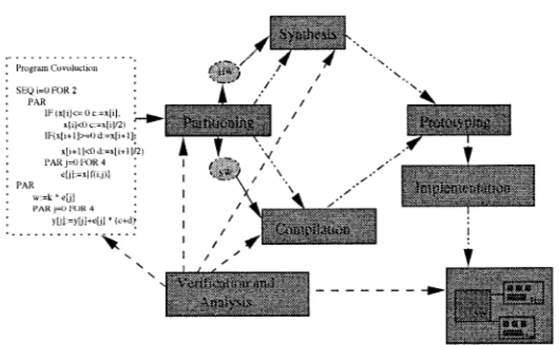
The PISH co-design methodology being developed by a research group at Universidade de Pernambuco, uses occam as its specification language and comprises all phases of the design process, as depicted in Figure 1. The occam specification is partitioned into a set of processes, where some sets are implemented in software and others in hardware. The partitioning is carried out in such a way that the partitioned description is formally proved to have the same semantics as the original one. The partitioning task is guided by the metrics computed in the analysis phase. Processes for communication purposes are also generated
Figure 1. PISH design flow.
in the partitioning phase. A more detailed description of the partitioning approach is given in Section 4.
After partitioning, the processes to be implemented in hardware are synthesized and the software processes are compiled. The technique proposed for software compilation is also formally verified [93]. For hardware synthesis, a set of commercial tools has been used. First system prototype has been generated by using two distinct prototyping environments: The HARP board developed by Sundance and a transputer plus FPGAs boards, both connected through a PC bus. Once the system is validated, either the hardware components or the whole system can be implemented as an ASIC circuit. For this purpose, layout synthesis techniques for Sea-of-gates technology have been used [94].
3. A Language for Specifying Communicating Processes
The goal of this section is to present the language which is used both to describe the appli-cations and to reason about the partitioning process itself. This language is a representative subset of occam, defined here by the BNF-style syntax definition showed below, where [clause] has the usual meaning of an optional item.
The optional argument rep stands for a replicator. A detailed description of these con-structors can be found in [62]. This subset of occam has been extended to consider two new constructors: BOX and CON. The syntax of these constructors is BOX P and CON P, where P is a process. These constructors have no semantic effect. They are just anno-tations, useful for the classification and the clustering phases. A process included within a BOX constructor is not split and its cost is analyzed as a whole at the clustering phase. The constructor CON is an annotation for a controlling process. Those processes act as an interface between the processes.
The occam subset is described in BNF format:
P: := SKIPkSTOPkx:=e nop, deadlock and assignment kch?x kch!e input and output
kIF(c1p1, . . . ,cnpn)kALT(g1p1, . . . ,gnpn)conditional and non-deterministic
conditional
kSEQ(p1, . . . ,pn)kPAR(p1, . . . ,pn)sequential and parallel combiners
kWHILE(c P)while loop kVAR x: P variable declaration kCHAN ch: P channel declaration
Occam obeys a set of algebraic laws [62] which defines its semantics. For example, the laws PAR(p1,p2)=PAR(p2,p1)and SEQ(p1,p2, . . . ,pn)=SEQ(p1,SEQ(p2, . . . ,pn))
define the symmetry of the PAR constructor and the associativity of the SEQ constructor, respectively.
4. The Hardware/Software Partitioning
Due to the computational complexity of optimum solution strategies, a need has arisen for a simplified, suboptimum approach to the partitioning system.
In [20, 14, 18, 10, 11] some heuristic algorithms to the partitioning problem are presented. Recently, some works [12, 13] have suggested the use of formal methods for the partitioning process. However, although these approaches use formal methods to hardware/software partitioning, neither of them includes a formal verification that the partitioning preserves the semantics of the original description.
The work reported in [16] presents some initial ideas towards a partitioning approach whose emphasis is correctness. This was the basis for the partitioning strategy presented here. As mentioned, the proposed approach uses occam [62] as a description language and suggests that the partitioning of an occam program should be performed by applying a series of algebraic transformations into the program. The main reason to use occam is that, being based on CSP [60], occam has a simple and a elegant semantics, given in terms of algebraic laws. In [63] the work is further developed, and a complete formalization of one of the partitioning phases, the splitting, is presented.
The main idea of the partitioning strategy is to consider the hardware/software partition-ing problem as a program transformation task, in all its phases. To accomplish this, an extended strategy to the work proposed in [16] has been developed, adding new algebraic transformation rules to deal with some more complex occam constructors such as replica-tors. Moreover, the proposed method is based on clustering and takes into account multiple software components.
The partitioning method uses Petri nets as a common formalism [41] which allows for a quantitative analysis in order to perform the partitioning, as well as the qualitative analysis of the systems so that it is possible to detect errors in an early phase of the design [33].
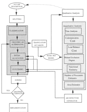
Figure 2. Task diagram.
4.1. The Partitioning Approach: An Overview
This section presents an overview of our proposed partitioning approach. The partitioning method is based on clustering techniques and formal transformations; and it is guided by the results of the quantitative analysis phase [61, 69, 70, 72, 73, 75]. The task-flow of the partitioning approach can be seen in Figure 2. This work extends the method presented in [15] by allowing to take into account a more generic target architecture. This must be defined by the designer by using the architecture generator, a graphical interface for specifying the number of software components, their interconnection as well as the memory organisation. The number and architecture of each hardware component will be defined during the partitioning phase.
The first step in the partitioning approach is the splitting phase. The original description is transformed into a set of concurrent simple processes. This transformation is carried out by applying a set of formal rewriting rules which assures that the semantics is preserved [63]. Due to the concurrent nature of the process, communication must be introduced
among sequential data dependent processes. The split of the original description in simple processes allows a better exploration of the design space in order to find the best partitioning. In the classification phase, a set of implementation alternatives is generated. The set of implementation alternatives is represented by a set of class values concerning some features of the program, such as degree of parallelism and pipeline implementation. The choice of some implementation alternative as the current one can be made either manually or automatically. When choosing automatically, the alternatives lead to a balanced degree of parallelism among the various statements and the minimization of the area-delay cost function.
Next, the occam/timed Petri net translation takes place. In this phase the split program is translated into a timed Petri net.
In the qualitative analysis phase, a cooperative use of reduction rules, matrix algebra approach and reachability/coverability methods is applied to the Petri net model in order to analyze the properties of the description. This is an important aspect of the approach, because it allows for errors to be detected in an early phase of the design and, of course, decreases the design costs [33].
After that, the cost analysis takes place in order to find a partition of the set of processes, which fulfills the design constraints. In this work, the quantitative analysis is carried out by taking into account the timed Petri net representation of the design description, which is obtained by a occam/timed Petri net translation tool. Using a powerful and formal model such as Petri nets as intermediate format allows for the formal computation of metrics and for performing a more accurate cost estimation. Additionally, it makes the metrics computation independent of a particular specification language. In the quantitative analysis, a set of methods for performance, area, load balance and mutual exclusion estimation have been developed in the context of this work. The results of this analysis are used to reason about alternatives for implementing each process.
After this, the initial allocation takes place. The term initial allocation is used to describe the initial assignment of one process to each processor. The criteria used to perform the initial allocation is the minimization of the inter-processor communication, balancing of the workload and the mutual exclusion degree among processes. One of the main problems in systems with multiple processors is the degradation in throughput caused by saturation effects [68, 66]. In distributed and multiple processor systems [65, 67], it is expected that doubling the number of processors would double the throughput of the system. However, experience has showed that throughput increases significantly only for the first few additional processors. Actually, at some point, throughput begins to decrease with each additional processor. This decrease is mainly caused by excessive inter-processor communication. The initial allocation method is based on a clustering algorithm.
In the clustering phase, the processes are grouped in clusters considering one implemen-tation alternative for each process. The result of the clustering process is an occam descrip-tion representing the obtained clustering sequence with addidescrip-tional informadescrip-tion indicating whether processes kept in the same cluster should be serialized or not. The serialization leads to the elimination of the unnecessary communication introduced during the splitting phase. A correct partitioned description is obtained after the joining phase, where transformation rules are applied again in order to combine processes kept in the same cluster and to eliminate
communication among sequential processes. In the following each phase of the partitioning process is explained with more detail.
4.2. The Splitting Strategy
As mentioned, the partitioning verification involves the characterization of the partitioning process as a program transformation task. It comprises the formalization of the splitting and joining phases already mentioned.
The goal of the splitting phase is to permit a flexible analysis of the possibilities for com-bining processes in the clustering phase. During the splitting phase, the original description is transformed into a set of simple processes, all of them in parallel. Since in occam PAR is a commutative operator, combining processes in parallel allows an analysis of all the permutations. The simple processes obey the normal form given below.
chanch1,ch2, . . . ,chn: PAR(P1,P2, . . . ,Pk)
where each Pi, 1<i <k is a simple process.
Definition 4.1 (Simple Process). A process P is defined as a simple if it is primitive
(SKIP,STOP,x:=e,ch ? x,ch ! e), or has one of the following forms: (i.) ALT(b,&gkck:=
true)(ii.) IF(bkck:=true)(iii.) BOX Q, HBOX Q and SBOX Q, where Q is an arbitrary
process. (iv.) IF(c Q,TRUE SKIP)where Q is primitive or a process as in (i), (ii) or (iii). (v.), where Q is simple and are communication commands, possibly combined in sequence or in parallel. (vi.) WHILE c Q, where Q is simple. (vii.) VAR x: Q, where Q is simple. (viii.) CON Q, where Q is simple.
This normal form expresses the granularity required by the clustering phase and this transformation permits a flexible analysis of the possibilities for combining processes in that phase. In [63] a complete formalization of the splitting phase can be found.
To perform each one of the splitting and joining phases, a reduction strategy is necessary. The splitting strategy developed during the PISH project has two main steps.
1. the simplification IF and ALT processes
2. the parallelisation of the intermediary description generated by Step 1.
The goal of Step 1 is to transform the original program into one in which all IFs and ALTs are simple processes. To accomplish this, occam laws have been applied. Two of these rules can be seen in Figure 3. The Rule 4.1.1 deals with conditionals. This rule transforms an arbitrary conditional into a sequence of IFs, with the aim to achieve the granularity required by the normal form. The application of this rule allows a flexible analysis of each sub-process of a conditional in the clustering phase.
Note that the role of the first IF operator on the right-hand side of the rule above is to make the choice and to allow the subsequent conditionals to be carried out in sequence. This is why the fresh variables are necessary. Otherwise, execution of one conditional can interfere
Figure 3. Two splitting rules.
in the condition of a subsequent one. After Step 1, all IFs and ALTs processes are simple, but not necessarily PAR, SEQ and WHILE processes. To be simple, the sub-process of a conditional is either a primitive process or can include only ALT, IF and BOX processes. Rule 4.1.2 distributes IF over SEQ and guarantees that no IF will include a SEQ operator as its internal process.
The goal of Step 2 is to transform the intermediate description generated by Step 1 into a simple form stated by the definition given above where all processes are kept in parallel. This can be carried out by using four additional rules. Rule 2 is an example of these rules, which puts in parallel two original sequential processes.
In this rule, z is a list of local variables of S E Q(P1,P2), x1is a list of variables used and
assigned in Piand xi0is a list of variables assigned in Pi. Assigned variables must be passed
because one of Pi may have a conditional command including an assignment that may or
not be executed.
The process annotated with the operator CON is a controlling process, and this operator has no semantic effect. It is useful for the clustering phase. This process acts as an interface between the processes under its control and the rest of the program. Observe that the introduction of local variables and communication is essential, because processes can originally share variables (the occam language does not allow variable sharing between parallel processes). Obviously, there are other possible forms of introducing communication than that expressed in Rule 2. This strategy, however, allows for having control of the introduced communication, which makes the joining phase easier.
Moreover, although it may seem expensive to introduce communication into the system, this is really necessary to allow a complete parallelisation of simple processes. The joining phase must be able to eliminate unnecessary communication between final processes. After the Step 2, the original program has been transformed into a program obeying the normal form.
4.3. The Partitioning Algorithm
The technique for hardware/software process partitioning is based on the approach proposed by Barros [14, 15], which includes a classification phase followed by clustering of processes. These phases will be explained with more detail in this section. The considered version of such an approach did not cope with hierarchy in the initial specification, and only fixed size loops had been taken into account in the cost analysis. Additionally, the underlying architecture template considered only one software component (i.e. only one microprocessor or microcontroller), which limits the design space exploration. This work addresses some of these lacks by using Petri nets as an intermediate format, which support abstraction concepts and provide a framework for an accurate estimation of communication, area and delay cost, as well as load balance and mutual exclusion between processes. Additionally, the partitioning can taken into account more complexes architectures, which can be specified by the designer through a graphical environment. The occam/Petri net translation method and the techniques for a quantitative analysis will be later explained, respectively.
4.3.1. Classification
In this phase a set of implementation possibilities represented as values of predefined attributes is attached to each process. The attributes were defined in order to capture the kind of communication performed by the process, the degree of parallelism inside the
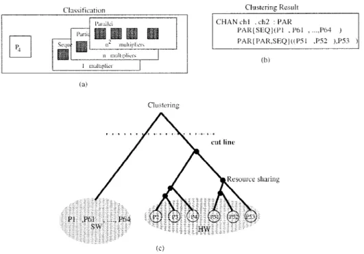
Figure 5. Classification and clustering phases.
process (PAR and REPPAR constructors), whether the assignments in the process could be performed in pipeline (in the case of REPSEQ constructor) and the multiplicity of each process. As an example, Figure 5a illustrates some implementation alternatives for the process, which has a REPPAR constructor. Concerning distinct degrees of parallelism, all assignments inside this process can be implemented completely parallel, partially parallel or completely sequential.
Although a set of implementation possibilities is attached to each process, only one is taken into account during the clustering phase and the choice can be done automatically or manually. In the case of an automatic choice, a balance of the parallelism degree of all implementations is the main goal.
4.3.2. The Clustering Algorithm
Once a current alternative of implementation for each process has been chosen, the clustering process takes place. The first step is the choice of some process to be implemented in the software components. This phase is called initial allocation [74] and may be controlled by the user or may be automatically guided by the minimization of a cost function. Taking into account the Petri net model, a set of metrics is computed and used for allocating
one process to each available software component. The allocation is a very critical task, since the partitioning of processes in software or hardware clusters depends on this initial allocation. The developed allocation method is also based on clustering techniques and groups processes in clusters by considering criteria such as communication cost [69, 70], functional similarity, mutual exclusion degree [73] and load balancing [72]. The number of resulting clusters is equal to the number of the software components in the architecture. From each cluster obtained, one process is chosen to be implemented in each software component. In order to implementing this strategy, techniques for calculating the degree of mutual exclusion between processes, the work load of processors, the communication cost and the functional similarity of processes have been defined and implemented.
The partitioning of processes has been performed using a multi-stage hierarchical clus-tering algorithm [74, 15]. First a clusclus-tering tree is built as depicted in Figure 5.b. This is performed by considering criteria like similarity among processes, communication cost, mutual exclusion degree and resource sharing. In order to measure the similarity between processes, a metric has been defined, which allows for quantifying the similarity between two processes by analyzing the communication cost, the degree of parallelism of their cur-rent implementation, the possibility of implementing both processes in pipeline and the multiplicity of their assignments [15]. The cluster set is generated by cutting the clustering tree at the level (see Figure 5.b), which minimizes a cost function. This cost function considers the communication cost as well as area and delay estimations [75, 72, 61, 59, 15]. Below a basic clustering algorithm is described. First, a clustering tree is built based on a distance matrix. This matrix provides the distance between each two objects:
p1p2 p3 p4 D = 0 d1 d2 d3 p1 0 d4 d5 p2 0 d6 p3 0 p4 Algorithm
1. Begin with a disjoint clustering having level L(0)=0 and sequence number m=0. 2. Find the least dissimilar pair r , s of clusters in the current clustering according to
d(r,s)=mi n{d(oi,oj)}.
3. Increment the sequence number(m ← m+1). Merge the clusters r and s into a simple one in order to form the next clustering m. Set the level of this clustering to L(m)=d(r,s).
4. Update the distance matrix by deleting the row and the column corresponding to the clusters. The distance between the new cluster and an old cluster k may be de-fined as: d(k, (r,s))=Max{d(k,r),d(k,s)}, d(k, (r,s))=Mi n{d(k,r),d(k,s)}or d(k, (r,s))=Average{d(k,r),d(k,s)}.
After the construction of the clustering tree, this tree is cut by a cut-line. The cut-line makes clusters according to a cut-function.
In order to allow the formal generation of a partitioned occam description in the joining phase, the clustering output is an occam description with annotations, which reflects the structure of the clustering tree, indicating whether resources should be shared or not.
4.4. The Joining Strategy
Based on the result of the clustering and on the description obtained in the splitting, the joining phase generates a final description of the partitioned program in the form:
chan: ch1,ch2, . . . ,chn: PAR(S1, . . . ,Ss,H1, . . . ,Hr)
where each Siand Hjare the generated clusters. Each of these is either one simple process (Pk)of the split phase of a combination of some(Pk)’s. Also, none of the(Pk)’s is left out:
each one is included in exactly one cluster. In this way, the precise mathematical notion of partition is captured. The Si, by convention, stands for the a software process and each Hj
for a hardware process.
Like the splitting phase, the joining phase should be designed as a set of transforma-tion rules. Some of these rules are simply the inverses of the ones used in the splitting phase, but new rules for eliminating unnecessary communication between processes of a same cluster have been implemented [63]. The goal of the joining strategy is to elim-inate irrelevant communication in the same cluster and after joining branches of condi-tionals and ALT processes as well as reducing sequences of parallel and sequential pro-cesses.
The joining phase is inherently more difficult than splitting. The combination of simple processes results in a process which is not simple anymore. Therefore, no obvious normal form is obtained to characterize the result of the joining in general. Also, one must take a great care for not introducing deadlock when serializing processes in a given cluster. Also, in this phase some sequential processes are carried out in parallel, by applying some transformation rules.
5. A Brief Introduction to Petri Nets
Petri nets are a powerful family of formal description techniques with a graphic and mathe-matical representation, and have powerful methods which allow for performing qualitative and quantitative analysis [37, 28, 29, 64].
This section presents a brief introduction to Place/Transitions nets and Timed Petri nets.
5.1. Place/Transition Nets
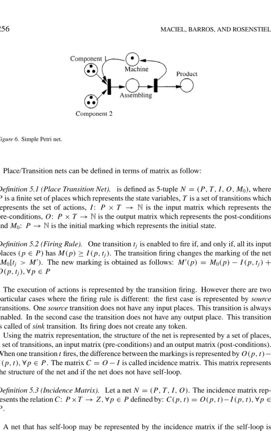
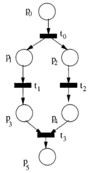
Place/Transition Nets are bipartite graphs represented by two types of vertices called places (circles) and transitions (rectangles), interconnected by directed arcs (see Figure 6).
Figure 6. Simple Petri net.
Place/Transition nets can be defined in terms of matrix as follow:
Definition 5.1 (Place Transition Net). is defined as 5-tuple N =(P,T,I,O,M0), where P is a finite set of places which represents the state variables, T is a set of transitions which represents the set of actions, I : P ×T → Nis the input matrix which represents the pre-conditions, O: P×T →Nis the output matrix which represents the post-conditions and M0: P →Nis the initial marking which represents the initial state.
Definition 5.2 (Firing Rule). One transition tjis enabled to fire if, and only if, all its input
places(p∈ P)has M(p)≥I(p,tj). The transition firing changes the marking of the net (M0[tj > M0). The new marking is obtained as follows: M0(p) = M0(p)−I(p,tj)+
O(p,tj),∀p∈ P
The execution of actions is represented by the transition firing. However there are two particular cases where the firing rule is different: the first case is represented by source transitions. One source transition does not have any input places. This transition is always enabled. In the second case the transition does not have any output place. This transition is called of sink transition. Its firing does not create any token.
Using the matrix representation, the structure of the net is represented by a set of places, a set of transitions, an input matrix (pre-conditions) and an output matrix (post-conditions). When one transition t fires, the difference between the markings is represented by O(p,t)− I(p,t),∀p∈ P. The matrix C=O−I is called incidence matrix. This matrix represents the structure of the net and if the net does not have self-loop.
Definition 5.3 (Incidence Matrix). Let a net N =(P,T,I,O). The incidence matrix rep-resents the relation C: P×T →Z,∀p∈ P defined by: C(p,t)=O(p,t)−I(p,t),∀p∈ P.
A net that has self-loop may be represented by the incidence matrix if the self-loop is refined using dummy pair [37].
The state equation describes the behavior of the system, as well as allows for the analysis of properties of the models. Using matrix representation, the transition tjis represented by
a vector s, where the components of the vector are zero except for the j−t h component, which is one. So it is possible to represent a marking either as
M0(p)=M0(p)−I(p,tj)+O(p,tj)
or as
M0(p) = M0(p)−I.s(tj)+O.s(tj)
= M0(p)=M0(p)−C.s(tj)T,∀p∈ P.
Applying the sequence sq=t0, . . . ,tk, . . . ,t0, . . . ,tnof transitions to the equation above,
the following equation is obtained
M0(p)=M0(p)+C.s¯,
wheres¯=s(t0)T,s(t1)T, . . . ,s(tn)T is called Parikh vector.
The Place/Transition nets can be divided into several classes [28]. Each class has distinct modeling power. The use of subclasses improves the decision power of the models, although without excessively decreasing the modeling power.
5.2. Analysis
The methods used to analyze Petri nets may be divided into three classes. The first method is graph-based and it builds on the reachability graph (reachability tree). The reachability graph is initial marking dependent and so it is used to analyse behavioral properties [39]. The main problem in the use of reachability tree is the high computational complexity [43, 44, 45, 46, 47, 48, 49, 50, 51, 52, 53, 54, 55] even if some interesting techniques are used such as: reduced graphs, graph symmetries, symbolic graph etc [35, 36]. The second method is based on the state equation [34, 37, 84, 86]. The main advantage of this method over the reachability graph is the existence of simple linear algebraic equations that aid in determining properties of the nets. Nevertheless, it gives only necessary or sufficient condition to the analysis of properties when it is applied to general Petri nets. The third method is based on reduction laws [37, 38]. The reduction laws based method provides a set of transformation rules which reduces the size of the models, preserving the properties. However, it is possible that for a given system and some set of rules, the reduction can not be complete.
From a pragmatic point of view, it is fair to suggest that a better, more efficient and more comprehensive analysis can be done by a cooperative use of these techniques. Nevertheless, necessary and sufficient conditions can be obtained by applying the matrix algebra for some subclasses of Petri nets [33].
5.3. Timed Petri Nets
So far, Petri nets have been used to model a logical point of view of the systems; no formal attention has been given to temporal relations and constraints [71, 78, 76]. The first temporal approach was proposed by Ramchandani [57]. Today, there are at least three approaches which associate time to the nets: stochastic, firing times specified by intervals and deterministic. In the stochastic nets a probability distribution to the firing time is assigned to the model [80, 79].
Time can be associated with places (Place-Timed Models) [83], tokens (Token-Timed Models) [82] and transitions (Transition-Timed Petri Models). The approach proposed in [71] associates to each transition a time interval (dmi n,dmax) (Transition-Time Petri Nets).
In deterministic timed nets the transitions firing can also be represented by policies: the first one is the three phase policy firing semantics and the second model is the atomic firing semantics approach. In the deterministic timed net with three phase policy semantics, the time information represents the duration of the transition’s firing [57]. The deterministic timed net with atomic firing may be represented by the approach proposed at [71] where time interval bounds are the same (di,di) (Transition-Time Petri Nets).
This section deals with the Timed Petri Nets, or rather, Petri net extensions in which the time information is expressed by duration (deterministic timed net with three phase policy firing semantics) and it is associated to the transitions.
Definition 5.4 (Timed Petri Nets). Let a pair N t =(N,D)be a timed Petri net, where N =(P,T,I,O,M0)is a Petri net, D: T →R+∪0, is a vector which associates to each transition tithe duration of the firing di.
A state in a Timed Petri Net is defined as 3-tuple of functions, one of which is the marking of the places; the second is the distribution in firing transitions and the last is the remaining firing time [77], for instance, if the number of tokens in a firing transition ti is mt(ti)=k,
then the remaining firing time is represented by a vector RT(t) = (r t(t)1, . . . ,r t(t)k).
More formally:
Definition 5.5 (State of Timed Petri Net). Let N t = (N,D)a Timed Petri Net, a state S of N t is defined by a 3-tuple S =(M,M T,RT), where M: P → Nis the marking, M T : T →Nis the distribution of tokens in the firing transitions and RT : K →R+T is the remaining firing time function which assigns the remaining firing time to each independent firing of a transition for each transition that mt(t) 6= 0. K is the number of tokens in a firing transition ti(mt(ti) = K). RT is undefined for the transitions ti which mt(ti) =
0.
A transition tiobtaining concession at a time x is obliged to fire at the time, if there is no
conflict.
Definition 5.6 (Enabling Rule). Let N t = (N,D) be a Timed Petri Net, and S =
x if, and only if, M(p)≥P∀ti∈BT#BT(ti)×I(p,ti),∀p ∈ P, where BT(ti)⊆BT and
#BT(ti)∈N.
If a bag of transitions BT is enabled at the instant x, thus at that instant it removes from the input places of the bag BT the corresponding number of tokens(#BT(ti)×I(p,ti))
and, at the time x+di(diis the duration related to the transition tiin the bag BT ), adds the
respective number of tokens in the output place. The number of tokens stored in the output place is equal to the product of the output arc weight(I(p,t))by the module of the bag regarding each transition t which has the duration equal to di(#BT(t),BT(t)⊆BT)plus
the number of tokens already “inside” the firing transitions, such that their duration have elapsed, during the present bag firing.
Definition 5.7 (Firing Rule). Let N t = (N,D) be a Timed Petri Net, and S =
(M,M T,RT) the state of N t . If a bag of transitions BT is enabled at the instant x, then at the instant xP∀ti∈BT#BT(ti)× I(p,ti),∀p ∈ P number of tokens is
re-moved from the input places of the bag BT . At the time x+d, the reached marking is M0=M−P∀t i∈BT#BT(ti)×I(p,ti)+ P ∀ti∈BT|di=d#BT(ti)×O(p,ti)+ P ∀tj∈T,M T(tj)>0 M(tj)×O(p,tj),∀p ∈ P, if no other transition t ∈ T has been fired in the interval (x,x+di).
The inclusion of time in the Petri net models allows for performance analysis of systems. Section 8 introduces performance analysis in a Petri net context paying special attention to structural approaches of deterministic models.
6. The Occam—Petri Net Translation Method
The development of a Petri net model of occam opens a wide range of applications based on qualitative analysis methods. To analyze performance aspects one requires a timed net model that represents the occam language.
In our context, an occam program is a behavioral description which has to be implemented combining software and hardware components. Thus, the timing constraints applied to each operations of the description is already known, taking into account either hardware or software implementation.
This section presents a timed Petri net model of occam language. This model allows for the execution time of the activities to be computed using the methods described in Sections 10 and 8.
The occam-Petri net translation method [61] receives an occam description and translates it into a timed Petri net model. The occam programming language is derived from CSP [60], and allows the specification of parallel algorithms as a set of concurrent processes. An occam program is constructed by using primitive processes and process combiners as described in Section 3.
The simplest occam processes are the assignment, the input action, the output action, the skip process and the stop process. Herewith, due to space restriction, only one primitive
Figure 7. Communication.
process as well as one combiner will be described. A more detailed description can be found in [59, 61, 64].
6.1. Primitive Communication Process: Input and Output
Occam processes can send and receive messages synchronously through channels by using input (?) and output (!) operations. When a process receives a value through a channel, this value is assigned to a variable.
Figure 7.b gives a net representing the input and the output primitive processes of the example in Figure 7.a. The synchronous communication is correctly represented by the net. It should be observed that the communication action is represented by the transition t0and is only fired when both the sender and the receiver processes are ready, which are
represented by tokens in the places p0and p1. When a value is sent by an output primitive
process through ch1, it is received and assigned to the variable x, being represented in the
net by the data part of the model. Observe that the transition t1can only be fired when the
places p2and p3 have tokens. After that, both processes become enabled to execute the
Figure 8. Parallel.
6.2. Parallelism
The combiner Par is one of the most powerful of the occam language. It permits concurrent process execution. The combined processes are executed simultaneously and only finish when every one has finished.
Figure 8.a shows a program containing two processes t1and t2. Figure 8.b shows a net
that represents the control of this program.
One token in the place p0 enables the transition t0. Firing this transition, the tokens
are removed from the input place(p0)and one token is stored in the output places ( p1
and p2). This marking enables the concurrent firings of the transitions t1 and t2. After
the firing of these transitions, one token is stored in the places p3 and p4, respectively.
This marking allows the firing of the transition t3, which represents the end of the parallel
execution.
7. Qualitative Analysis
This section depicts the proposed method to perform qualitative analysis. The quantitative analysis of behavioral descriptions is described in following sections.
Concurrent systems are usually difficult to manage and understand. Therefore, misun-derstanding and mistakes are frequent during the design cycle [87].
Therefore, a need arises to decrease the cost and time-to-market of the products. Thus, it is fair to suggest the formalization of properties of the systems so that it is possible to detect errors in an early phase of the design.
There are so many properties which could be analyzed in a Petri net model [37]. Among these properties, we have to highlight some very important ones in a control system context: boundedness, safeness, liveness and reversibility. Boundedness and safeness imply the absence of capacity overflow. For instance, there may be buffers and queues, represented by places, with finite capacity. If a place is bounded, it means that there will be no overflow. One place bounded to n means that the number of tokens that will be stored in it is at most n. Safeness is a special case of boundness: n equal to one. Liveness is related to the deadlock absence. Actually, if a system is deadlock free, it does not mean that the system is live, although if a system is live, it is deadlock free. This property guarantees that a system can successfully produce. One deadlock free system may also be not live, which is the case when a model does not have any dead state, but there exists at least one activity which is never executed. Liveness is a fundamental property in many real systems and also very complex to analyze in a broad sense. Therefore, many authors have been divided liveness in terms of levels in such a way to make it easy to analyze. Another very important property is reversibility. If a system is reversible, it means that this system has a cyclic behavior and that it can be initialized from any reachable state.
The analysis of large dimensions nets is not a trivial problem, therefore in the prag-matic point of view, a cooperative use of reduction rules, structural analysis and reachabil-ity/coverability methods is important.
The first step of the adopted analysis approach is the application of the ‘closure’ [32] by the introduction of a fictitious transition t, whose the time duration is 0. The second step should be the application of transformation rules which preserves properties like boundedness and liveness of the models. Such rules should be applied in order to reduce the model dimension. After that, the matrix algebra and the reachability methods can be applied in order to obtain the behavioral and the structural properties related to the model. Below, the sequence of steps adopted to carry out the qualitative analysis is depicted.
• Application of a ‘closure’ to the net by the introduction of the transition t , • Application of reduction rules to net,
• Application of structural methods and
• Application of reachability/coverability methods.
8. Performance Analysis
The calculation of execution time is a very important issue in hardware/software codesign. It is necessary for performance optimization and for validating timing constraints [3]. Formal performance analysis methods provide upper and/or lower (worst/best) bounds instead of a single value.
The execution time of a given program is data dependent and takes into account the actual instruction trace which is executed. Branch and loop control flow constructs result in an exponential number of possible execution paths. Thus, specific statistics must be collected by considering a sample data set in order to determine the actual branch and
loop counts. This approach, however, can be used only in probabilistic analysis. In some limited applications it is possible to determine the conditionals and loop iteration counts by applying symbolic data flow analysis.
Another important aspect is the cost of formal performance analysis. Performance anal-ysis does not intend to replace simulation; instead, besides a model for simulation, an accurate model for performance analysis must be provided.
Worst/best case timing analysis may be carried out by considering path analysis techniques [19, 6]. In worst/best case analysis, it has been assumed the worst/best case choices for each branch and loop. An alternative method allows the designer to provide simple execution number of certain statements. It helps to specify the total execution number of iteration of nested loops. Methods based on Max-Plus algebra have also been applied for performance evaluation, but for mean case performance it suffers of a great complexity and only works for some special classes of problems [81].
This section presents one technique for static performance analysis of behavioral descrip-tions based on structural Petri net methods. Static analysis is referred to as methods which use information collected at compilation time and may also include information collected in profiling runs [90].
Real time systems can be classified either as a hard real time system or a soft real time system. Hard real time systems cannot tolerate any missed timing deadlines. Thus, the performance metric of interest is the extreme case, typically the worst case, nevertheless the best case may also be of interest. In a soft real time system, a occasional missing timing deadline is tolerable. In this case, a probabilistic performance [80, 79, 89] measure that guarantees a high probability of meeting the time constraints suffices.
The inclusion of time in the Petri net model allows for performance analysis of systems [85]. Max-Plus algebra has been applied to Petri net models for system analysis [92], but such approaches can only be considered for very restricted Petri nets subclasses [5]. One very well known method for computing cycle time in Petri net is based on timed reachability graph with path-finder algorithm. However the computation of the timed reachability graph is very complex and for unbounded systems is infinite. The pragmatic point of view suggests exploring the structure (to transform or to model the systems in terms of Petri nets subclasses) of the nets and to apply linear programming methods [86].
Structural methods eliminate the derivation of state space, thus they avoid the “state explosion” problem of reachability based methods; nevertheless they cannot provide as much information as the reachability approaches do. However, some performance measures such as minimal time of the critical-path can be obtained by applying structural methods. Another factor which has influenced us to apply structural based methods is that every other metric used in our proposed method to perform the initial allocation and the partitioning is computed by using structural methods, or rather, the communication cost and the mutual exclusion degree computation algorithms are based on t-invariants and p-invariants methods. Firstly, this section presents an algorithm to compute cycle time for a specific deterministic timed Petri net subclass called Marked Graph [1]. After that, an extended approach is presented in order to compute extreme and average cases of behavioral description.
First of all, it is important to define two concepts: direct circuit and direct elementary circuits. A direct circuit is a directed path from one vertex (place or transition) back to
Figure 9. Timed marked graph.
itself. A directed elementary circuit is a directed circuit in which no vertices appear more than once.
THEOREM8.1 For a strongly connected Marked Graph N ,PM(pi)in any directed circuit
remains the same after any firing sequence s.
THEOREM 8.2 For a marked graph N , the minimum cycle time is given by Dm =
maxk{Tk/Nk}, for every circuit k in the net. Where Tk is the sum of every transition
delays in a circuit k and Nk= P
M(pi)in a circuit.
To compute all directed circuit in the net, first we have to obtain all minimum p-invariants, then use them to compute the direct circuits.
Figure 9 shows a marked graph, adopted from [1], in which we apply the method described previously. The reader should observe that each place has only one input and output transition.
Applying very well known methods to compute minimum p-invariants [37, 84], these supports are obtained: sp1= {p0,p2,p4,p6}, sp2 = {p0,p3,p5,p6}, sp3 = {p1,p2,p4}
and sp4 = {p1,p3,p5}. After obtaining the minimum p-invariants, it is easy to compute
the directed circuits: c1= {p0,t1,p2,t2,p4,t4,p6,t5}, c2 = {p0,t1,p3,t3,p5,t4,p6,t5},
c3 = {p1,t1,p2,t2,p4,t4} and c4 = {p1,t1,p3,t3,p5,t4}. The cycle time associated
to each circuit is: Dm(N) = max{T(1),T(2),T(3),T(4),T(5),T(6)}. Therefore, the
minimum cycle time is the Dm=maxk{12,16,10,12} =16.
If instead of using a Petri net model in which the delay related to each operation is attached to the transition, a Petri net model was adopted in which each transition has a time interval
(tmi n,tmax)attached to it (see Section 5.3), we may compute the lower bound of the cycle
time. Note that if the delay related to each transition is replaced by the lower bound(tmi n)
Herewith a structural approach is presented to computing extreme and average cases of behavioral description. The algorithm presented computes the minimal execution time, the minimal critical-path time and likely minimal time related to branch probabilities in partially repetitive or consistent strongly connected nets covered by p-invariants. This approach is based on the method presented previously, however it is not restricted only to marked graphs.
First, we present some definitions and theorems in Petri net theory which are important for the proposed approach [37].
A Petri net N is said to be repetitive if there is a marking and a firing sequence from this marking such that every transition occurs infinitely often. More formally:
Definition 8.1 (Repetitive net). Let N=(R;M0)be a marked Petri net and firing sequence s. N is said to be repetitive if there exists a sequence s such that M0[s>Mievery transition
ti ∈T fires infinitely often in s.
THEOREM8.3 A Petri net N is repetitive if, and only if, there exists a vector X of positive integers such that C·X≥0, X 6=0.
A Petri net is said to be consistent if there is a marking and a firing sequence from this marking back to the same marking such that every transition occurs at least once. More formally:
Definition 8.2 (Consistent net). Let N =(R;M0)be a market Petri net and firing sequence s. N is said to be consistent if there exists a sequence s such that M0[s>M0every transition
ti ∈T fires at least once in s.
THEOREM8.4 A Petri net N is consistent if, and only if, there exists a vector X of positive integers such that C·X=0, X 6=0.
The proofs of such theorems can be found in [37].
The method presented previously is based on the computation of the direct circuit by using the p-minimum invariants. In other words, first the p-minimum invariants are computed, then, based on these results, the direct circuits are computed (sub-nets). The cycle time related to a marked graph is the maximum delay considering each circuit of the net.
This method cannot be applied to nets with choices because the circuits which are com-puted by using the minimum p-invariants will provide sub-nets such that the simple summa-tion of the delays, attached to each transisumma-tion, gives a number representing all those branches of the choice. Another aspect which has to be considered is that concurrent descriptions with choice may lead to a deadlock. Thus, we have to avoid these paths in order to compute the minimal execution time of the model.
In this method we use the p-minimum invariants in order to compute the circuits of the net and the t-minimum invariants to eliminate from the net transitions which do not appear in any t-invariant. With regard to partially consistent models, these transitions are never
fired. We also have to eliminate from the net every transition which belongs to a choice, in the underlined untimed model, it does not model a real choice in the timed model. For instance, consider a net in which we have the following output bag related to the place pk: O(pk) = {ti,tj}. Thus, in the underlined untimed model these transitions describe
a choice. However, if in the timed model these transition have such time constraints: di
and dj and dj > di, a conflict resolution policy is applied such that transition ti must
be fired. After obtaining this new net (a consistent net), each sub-net obtained by each p-minimum invariant must be analyzed. In such nets, their transitions have to belong to only one t-minimum invariant. The sub-nets which cannot satisfy this condition have to be decomposed into sub-nets such that their transitions should belong to only one t-invariant. The number of sub-nets obtained has to be the minimum, or rather, the number of transitions of each sub-net in each t -invariant should be the maximum.
Definition 8.3 (Shared Element). Let N=(P,T,I,O)be a net, two subnets S1,S2⊂N ,
a set of places P0such that∀pz∈ P0,pz6∈ S1,pz6∈ S2. The set of places P0is said to be a
shared element if, and only if, its places are strongly connected and∃pm∈ P0,ti ∈S1,tk∈
S2such that ti,tk∈ O(pm)and∃pl∈ P0,tj ∈S1,tr ∈S2such that tj,tr ∈ I(pl).
THEOREM 8.5 Let N = (P,T,I,O)be a pure strongly connected either partially con-sistent or concon-sistent net covered by p-invariants without shared elements, S Nk ⊂ N
a subnet obtained from a p-minimum invariant I pi and covered by one t-minimum
in-variant I tj,S Nc ⊂ N a subnet obtained from a p-minimum invariant I pi and does not
covered by only one t-minimum invariant I tj and if ∃pk such that #O(pk) > 1 then
6 lj > hi,∀ti,tj ∈ O(pk). The time related to the critical path of the net N is given
by C T(N)=max{dS Nk,dS Nj},∀S Nk,S Nj ⊂N , where S Nj is obtained by a decomposi-tion of S Ncsuch that each S Nj ⊂S Ncis covered by only one t-minimum invariant.
THEOREM 8.6 Let N = (P,T,I,O)be a pure strongly connected either partially con-sistent or concon-sistent net covered by p-invariants without shared elements, S Nk ∈ N be
a subnet obtained from a p-minimum invariant I pi and covered by one t-minimum
in-variant I tj,S Nc ∈ N be a subnet obtained from a p-minimum invariant I pi and not
covered by only one t-minimum invariant I tj and if ∃pk such that #O(pk) > 1 then
6 ∃lj >hi,∀ti,tj ∈o(pk). Each S Nj ⊂S Ncis covered by only one t-minimum invariant,
where S Njis obtained by a decomposition of S Nc. The minimal time of the net N is given by
M T(N)=max{dS Nk,dS Nc},∀S Nc⊂N such that each dS Nc =mi n{dS Nj},∀S Nj ⊂S Nc. The proof of both theorems can be found in [72].
It is important to stress that the main difference among these metrics is related to the execution time of pieces of program in which choices must be considered. The computation of the minimal time related to the whole program takes into account the choice branch which provides the minimum delay.
Another important measure is the likely minimal time. This metric takes into ac-count probabilities of branches execution. Therefore, based on specific collected
statis-tics, the designer may provide, for each branch in the description, the probability of execution.
Definition 8.4 (Strongly Connected Component Probability Matrix). Let a net N =
(P,T,I,O,D), a strongly connected component S Nk ⊂ N be a branch bi related to a
choice-net. SC P M(S Nk,tj)is the execution probability of the transition tj in the strongly
connected component S Nk. SC P M(S Nk,tj): N×N→ 0 if tj ∈/ S Nk. pri(0≤R≤1) if tj ∈S Nk,tj ∈bi. 1 if tj ∈S Nk,tj ∈/ bi,∀bi ∈S Nk.
Definition 8.5 (Probability Execution Vector). Let a net N=(P,T,I,O,D)and a strongly connected component probability matrix SC P M related to N . P E V(tj):N→0≤R≤1,
#P E V(tj)=T . Each vector component pev(tj)= Q
∀S Nk SC P M(S Nk,tj),∀tj ∈T . The likely minimal time related to the net N is given by M L T =max{mltS Nk},∀S Nk, where mltS Nk =
P
d(tj)×pev(tj),∀tj∈ S Nk. d(tj)is the lower bound time related to the
transition tjand S Nkis a strongly connected component.
Similar results are obtained for either partially repetitive or repetitive nets covered by p-invariants. In nets with these properties, instead of computing the t-minimum invariants we have to compute the support of the equation systems C·X ≥0,X 6=0.
The algorithm to compute the minimal time, the minimal critical path time and likely minimal time is given in the following:
• Input:
a net N =(P,T,I,O,D).
branch probabilities bi = {pri;tj},∀bi ⊂N and∀tj ∈bi.
• Output:
the minimal time.
the minimal critical path time. the likely minimal time.
• Algorithm:
1. Compute the t-minimum invariants(I t)of the net N .
2. Remove from the net N the transition tl and the places pg ∈ I(tl)or pg ∈ O(tl),
if i t1 = 0,∀I t , such that: N0 =(P0,T0,I0,O0), where P0 = P\pg,pg ∈ I(tl)
and/or pg∈ O(tl)and T0=T\tl.
3. Compute the p-minimum invariants(I p)of the net N0. 4. Compute the probability execution vector(P E V).
5. Compute the likely execution time of each component S NP k ⊂ N0(mltS Nk = d(tj)×pev(tj),∀tj ∈ S Nk).
Figure 10. Example.
6. Compute the strongly connected components S Nkobtained from I pk.
7. Compute the strongly connected components S Nk0obtained from I pkand covered
by one t-minimum invariant I t .
8. For each strongly connected component (obtained from I pk) not covered by a
t-minimum invariant(S Nc0), do:
Decompose S Nc0into nets(S Nj0s)in such a way that a t-minimum invariant I tj covers each subnet S Nj0.
9. Compute the execution time of each component S Nk0,S Nj0 ⊂S Nc∀S Nk0,S Nj0 ∈
N0.
10. Compute the critical path time C T(N)=C T(N0)=max{dS Nk0,dS N0j} ∀S Nk0,S Nj0∈
N0.
11. Compute the minimal time M T(N)=M T(N0)=max{dS Nk0,dS NC0} ∀S Nk0,S NC0 ∈
N0and dS Nc0 =mi n{dS Nj0},∀S N 0
j ⊂S Nc0.
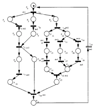
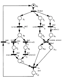
12. Compute the likely minimal time M L T(N)=max{mltS Nk},∀S Nk∈ N0. The method presented is applied to a small example (see Figure 10). This example is a concurrent description in which there are two choices. It is important to emphasize that one of these leads to a deadlock. In the qualitative analysis phase, we found out that the model is strongly connected, partially consistent, covered by semi-positive p-invariants, structurally bounded and safe.
Figure 11. Transformed net.
If the system is partially consistent, it means that some of its transitions either are not able to be fired or, if they were fired, they would lead to a deadlock.
The first step of the algorithm is the computation of the t-minimum invariant. The support of the t-minimum invariants are st1 = {t0,t2,t6,t7,t8,t9,t10,t11,t12,t13,t14,t15,t17}and
st2 = {t0,t2,t6,t7,t8,t9,t10,t11,t12,t13,t14,t16,t18}. By analyzing these invariants it may
be observed that the transitions t1,t3,t4,t5do not belong to any t-minimum invariant.
The second step is the elimination of the transitions which do not belong to any t-minimum invariant and also the elimination of the places that are input and/or output of such transitions. The resulting net (obtained by this transformation) is presented in Figure 11.
Considering the transitions of the branches of the choice (transitions t11,t16,t17and t18),
an execution probability of 0.5 was assigned.
The following step is the computation of the p-minimum invariants of the transformed net. The support of the p-minimum invariants are: sp1 = {p0,p1,p5,p8,p16,p18},
sp2 = {p0,p3,p12,p15,p17,p18,p19,p20}, sp3 = {p0,p1,p5,p10,p18}, sp4 = {p0,p2,
p9,p10,p18}, sp5 = {p0,p2,p8,p9,p16,p18}and sp6 = {p0,p3,p11,p13,p14,p17,p18}.
After that, the strongly connected components (Subneti) are obtained from these
in-variants. Each component has the following transitions as its elements: Subnet1 =
t13,t14}, Subnet4 = {t0,t6,t8,t13,t14}, Subnet5 = {t0,t6,t7,t8,t13,t14}and Subnet6 =
{t0,t9,t10,t11,t12,t13,t14,t15}.
Then, the likely minimal time for each strongly connected component mlt(S Nk) = P
d(tj)×pev(tj),∀tj ∈ S Nk): mlt(1) =12, mlt(2)=21, mlt(3)=7, mlt(4)=10,
mlt(5)=15 and mlt(6)=8 is computed
Each component which is not covered by only one t-minimum invariant is decomposed into subnets in such a way that each of its subnets is covered by only one t-minimum invariant. Therefore, the Subnet2 = {t0,t10,t11,t12,t13,t14,t16,t17,t18}is decomposed
into Subnet21= {t0,t10,t11,t12,t13,t14,t17}and Subnet22 = {t0,t10,t12,t13,t14,t16,t18}.
After that, we compute the time related to each subnet of the whole model. The result-ing values are: T(1)=12, T(21)=20, T(22)=22, T(3)=7, T(4)=10, T(5)=15 and T(6)=8. Then, we have C T(N)=max{T(1),T(21),T(22),T(3),T(4),T(5),T(6)} = 22,M T(N)=max{T(1),mi n{T(21),T(22)},T(3),T(4),T(5),T(6)} =20 and finally M L T(N)=max{mlt(1),mlt(2),mlt(3),mlt(4)mlt(5),mlt(6)} =21
For execution time computation in systems with data dependent loops, the designer has to assign the most likely number of iterations to the net. This number could be determined by a previous designer’s knowledge, therefore he/she may directly associate a number using annotation in the net. Another possibility is by simulating the net on several sets of samples and recording how often the various loops were executed.
Such a method has been applied to several examples and compared to the results obtained by the petri net tool INA. The results are equivalents, but INA only provides the minimal time.
9. Extending the Model for Hardware/Software Codesign
This section presents a method for estimating the necessary number of processors to execute a program, taking into account the resource constraints (number of processors) provided by the designer, in order to achieve best performance, disregarding the topology of the interconnection network.
First, let us consider a model extension in order to capture the number of proces-sors of the proposed architecture. The extended model is represented by the net N =
(P,T,I,O,M0,D), which describes the program, a set of places P0 in which each of its places(p0)is a processor type adopted in the proposed architecture; the marking of each of these places represents the number of processors of the type p0; the input and the output arcs that interconnect the places of the set P0to the transitions which represents the arithmetic/logical operations(ALUop⊂T).
In the extended model the number of conflicts in the net increases due to the competition of operations for processors [32]. These conflicts require the use of a pre-selection policy by assigning equal probabilities to the output arcs from processors places to the enabled transitions tj ∈ ALUop(O(p,tj),p ∈ P0)in each reachable marking Mz. Thus, more
formally:
Definition 9.1 (Extended Model). Let a net N=(P,T,I,O,M0,D)a program model, a set of places P0the processor types adopted in the architecture such that P∩P0= ∅and