Hybrids of Generative and Discriminative Methods for Machine Learning

Hybrids of Generative and

Discriminative Methods for

Machine Learning

Julia Aur´elie Lasserre

Queens’ College

University of Cambridge

This dissertation is submitted for the degree of Doctor of Philosophy.

March 2008

In machine learning, probabilistic models are described as be-longing to one of two categories: generative or discriminative. Generative models are built to understand how samples from a particular category were generated. The category chosen for a new data-point is the category whose model fits the point best. Discriminative models are concerned with defining the boundaries between the categories. The category chosen for a new data-point then depends on which side of the boundary it belongs to.

While both methods have different / complementary advantages, they cannot be merged in a straightforward way. The challenge we wish to undertake in this thesis is to find rigorous models blending these two approaches, and to show that it can help find good solutions to various problems.

Firstly, we will describe an original hybrid model [50] that allows an elegant blend of generative and discriminative approaches. We will show:

• how a hybrid approach can lead to better classification perfor-mance when most of the available data is unlabelled,

• how to make the optimal trade-off between the generative and discriminative extremes,

• and how the amount of labelled data influences the best model,

by applying this framework on various data-sets to perform semi-supervised classification.

Secondly, we will present a hybrid approximation of the belief prop-agation algorithm [51], that helps optimise a Markov random field of high cardinality. The contributions of this thesis on this issue are two-folded:

• a hybrid generative / discriminative method Hybrid BP that significantly reduces the state space of each node in the Markov random field,

• and an effective method for learning the parameters which ex-ploits the memory savings provided by Hybrid BP.

We will then see how reducing the memory needs and allowing the Markov random field to take higher cardinality was useful.

This dissertation is my own work and contains nothing which is the outcome of work done in collaboration with others, except as spec-ified in the text. Most of chapter 2 can be found in [50] and most of chapter 4 can be found in [51]. No part has been previously ac-cepted and presented for the award of any degree or diploma from any university.

This dissertation contains fewer than 45000 words and exactly 78 figures excluding the university crest on the title page. Therefore it stands within the authorised limits of 65000 words and 150 figures.

Firstly, I must express my deepest gratitude to my supervisor Prof Christopher Bishop. I have greatly benefitted from his experience, enthusiasm and advice. I also want to thank him for giving me the opportunity to experience Cambridge academic life under his wings.

I want to thank Prof Roberto Cipolla from the Department of Engineering for adopting me in his group half-way through my studies and for the help he has given me; Prof John Daugman from the Computer Laboratory for originally acccepting me in his group (and for managing my studentship!); Prof Zoubin Ghahramani and Prof Christopher Williams for accepting to examine me, and for giving me a gentle viva with many useful comments.

I am also immensely grateful to Microsoft Research Cambridge for their generous financial support, which has allowed me to do my studies in the best conditions possible.

I need to extend my sincere thanks to Dr Thomas Minka for his exciting ideas; to my friends Dr John Winn and Dr Anitha Kannan for a very educational, intense and fun internship at Microsoft Research Cambridge; and to all the people from my group whose help and company have made my working days so much more pleasant, in particular Gabe, Julien, Jamie, Tae-Kyun, Fabio, Bjorn, Carlos, George, and Matt J. I also want to mention all the people who have made my general experience in Cambridge so enjoyable: Matthias, Jim, Mair, Keltie, Jane, Sam, Matt D., my housemates Ben, Andreas, Roz, James, Catherine, Millie and Andrew, the Rhinos members, and the volleyball women’s Blues.

Last but not least, I would like to send my very tender thoughts to my close family in France. This thesis is dedicated to them. I want to give my encouragements to my adventurous sister Sarah - may she enjoy her dream-come-true to experience life in Japan; to my courageous sister Sophie - may she keep fighting hard in these diffi-cult times, I am confident she will find happiness on whichever path she will choose to pursue; and to my passionate brother Philippe -may he succeed in his wish to become a professional goal keeper.

Abstract i

Declaration ii

Statement of length iii

Acknowledgements v

List of figures xiii

Introduction 1

1 Generative or discriminative? 7

1.1 Generative models and generative learning . . . 8

1.2 Discriminative models and discriminative learning . . . 10

1.3 Generative vs discriminative models . . . 13

1.3.1 Different advantages . . . 13

1.3.2 Generative vs conditional learning . . . 16

1.3.3 Classification: Bayesian decision, point estimate . . . 18

1.4 Hybrid methods . . . 20

1.4.1 Hybrid algorithms . . . 20

Learning discriminative models on generative features . . . 21

Learning generative models on discriminative features . . . 22

Refining generative models with discriminative components . . . 22

Refining generative classifiers with a discriminative classifier . . . 23

Feature splitting . . . 24

When generative and discriminative models help each other out . . . 25

The wake-sleep-like algorithms . . . 26

1.4.2 Hybrid learning . . . 29

Discriminative training of generative models . . . 29

Convex combination of objective functions . . . 30

Multi-Conditional learning . . . 31

2.1.1 A new view of discriminative training . . . 36

2.1.2 Blending generative and discriminative models . . . 40

2.1.3 Illustration . . . 42

2.2 Comparison with the convex combination framework . . . 45

2.2.1 Visually . . . 46

2.2.2 Pareto fronts . . . 50

2.3 The Bayesian version . . . 54

2.3.1 Exact inference . . . 55

2.3.2 The true MAP . . . 56

2.3.3 Successive Laplace approximations . . . 61

First step . . . 62

Second step . . . 62

Results . . . 63

2.4 Conclusion . . . 68

3 Application to semi-supervised learning 69 3.1 The data-sets . . . 70

3.2 The features . . . 72

3.3 The underlying generative model . . . 73

3.4 The learning method . . . 76

3.5 Influence of the amount of labelled data . . . 81

3.5.1 On the generative / discriminative models . . . 82

General experimental set-up . . . 82

CSB data-set . . . 82

Wildcats data-set . . . 84

3.5.2 On the choice of model . . . 86

General experimental set-up . . . 90

CSB data-set - HF . . . 90

CSB data-set - CC . . . 94

Wildcats data-set - HF . . . 97

Wildcats data-set - CC . . . 100

3.5.3 On the choice between HF and CC . . . 103

CSB data-set . . . 103

Wildcats data-set . . . 103

3.5.4 Summary of the experimental results . . . 105

3.6 Discussion . . . 106

4 Hybrid belief propagation 111 4.1 Inference with belief propagation . . . 112

4.1.1 Standard belief propagation . . . 112

4.1.2 Approximations . . . 115

4.2 The Jigsaw model . . . 117

4.3.3 Hybrid belief propagation . . . 123

4.3.4 Efficiency of Sparse BP and Hybrid BP . . . 126

4.4 Hybrid learning of jigsaws . . . 130

4.4.1 Analysis of hybrid learning . . . 133

4.4.2 Image segmentation . . . 133

4.5 Discussion . . . 137

Conclusions 141 A Complements to chapter 2 147 A.1 Average plot for the toy example of section 2.1.3 . . . 147

A.2 Average plot for the toy example of section 2.2 . . . 149

A.3 Average plot for the toy example of section 2.3.2 . . . 150

A.4 Average plot for the toy example of section 2.3.3 . . . 151

B Complements to chapter 3 153 B.1 The trick . . . 153

B.2 The derivatives . . . 154

B.3 Results on the wildcats data-set with a mixture of 2 Gaussians . . . 157

B.3.1 Generative / discriminative models . . . 157

B.3.2 On the choice of model . . . 158

B.3.3 HF and CC . . . 165

1.1 Graphical representation of a basic generative model. . . 8

1.2 Training of a mixture of spherical Gaussians. . . 9

1.3 Graphical representation of a basic discriminative model. . . 11

1.4 Example of boundary obtained with an SVM. . . 12

1.5 Generative model vs discriminative model. . . 15

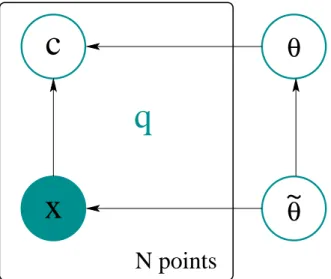
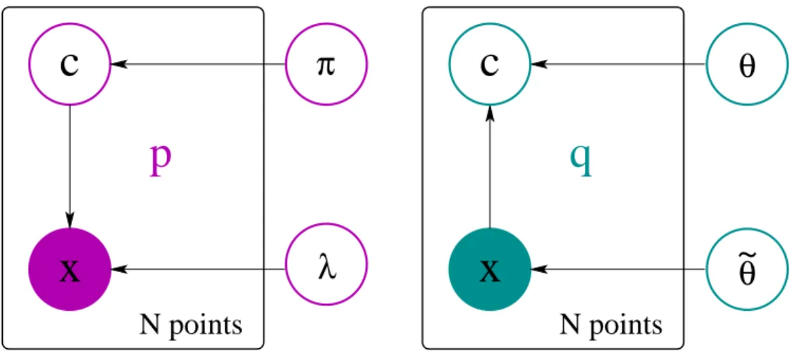
2.1 The additional set of parametersθ. . . .e 37 2.2 The communication channel is now open. . . 37

2.3 The discriminative case. . . 39

2.4 The generative case. . . 39

2.5 Hybrid models may do better. . . 40

2.6 Influence of the unlabelled data. . . 41

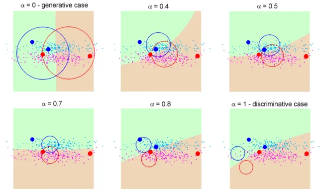
2.7 Synthetic training data. . . 43

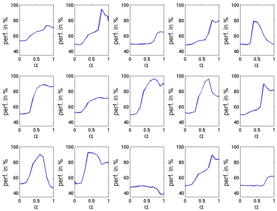
2.8 Classification performance of HF on the toy example for every run. . . 44

2.9 Results of fitting an isotropic Gaussian model to the synthetic data. . . 45

2.10 Classification performance of HF and CC on the toy example for every run. . 47

2.11 CC - run presenting similarities. . . 48

2.12 HF - run presenting differences. . . 49

2.13 CC - run presenting differences. . . 50

2.14 Visualisation of Pareto-optimal points. . . 51

2.15 Pareto fronts for both the HF and CC frameworks. . . 53

2.16 Pareto fronts for both the HF and CC frameworks. . . 54

2.17 Integrating overσ−2. . . 57

2.18 MAP approximation -b=a- run presented in figure 2.9. . . 58

2.19 MAP approximation -b= 1/2- run presented in figure 2.9. . . 59

2.20 Classification performance - MAP approximation - Gamma prior. . . 60

2.21 Laplace approximation - Gaussian prior - run presented in figure 2.9. . . 64

2.22 Laplace approximation - Gamma prior - run presented in figure 2.9. . . 65

2.23 Classification performance - Laplace approximation. . . 67

3.1 Sample images from the CSB data-set. . . 71

3.2 Sample images from the wildcats data-set. . . 71

3.3 The generative model for object recognition. . . 74

3.4 Other graphical models. . . 76

3.8 Schematic plots for the cumulative distribution function. . . 88

3.9 Schematic plots for the models’ probability. . . 89

3.10 CSB data-set - HF - Choice of model vs percentage of fully labelled data. . . . 91

3.11 CSB data-set - HF - Choice of model vs percentage of weakly labelled data. . 93

3.12 CSB data-set - CC - Choice of model vs percentage of fully labelled data. . . . 95

3.13 CSB data-set - CC - Choice of model vs percentage of weakly labelled data. . 96

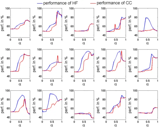
3.14 Wildcats data-set - HF - Choice of model vs percentage of fully labelled data. 98 3.15 Wildcats data-set - HF - Choice of model vs percentage of weakly labelled data. 99 3.16 Wildcats data-set - CC - Choice of model vs percentage of fully labelled data. 101 3.17 Wildcats data-set - CC - Choice of model vs percentage of weakly labelled data.102 3.18 CSB data-set - HF versus CC. . . 104

3.19 Wildcats data-set - HF versus CC. . . 105

3.20 Performance on the different runs. . . 107

4.1 A pair-wise 4-connected MRF. . . 113

4.2 Message passing. . . 114

4.3 The principle of sparse belief propagation. . . 116

4.4 Example the Jigsaw model applied to face images. . . 117

4.5 Diagram of the Jigsaw model. . . 118

4.6 Structure of the likelihood function. . . 119

4.7 Structure of the distribution of the label of a particular pixel. . . 120

4.8 Sparse structure of the messages. . . 122

4.9 The use of local evidence to favour mappings. . . 123

4.10 The use of local evidence to split similar pixels. . . 124

4.11 Role of the classifier. . . 125

4.12 Construction of the hybrid likelihood. . . 126

4.13 Segmentation on building images. . . 127

4.14 Various plots. . . 127

4.15 Recognition accuracy against memory use. . . 130

4.16 Memory needed for different jigsaw sizes. . . 131

4.17 Comparison of algorithms for learning jigsaws. . . 132

4.18 Accuracy of the hybrid learning against memory use. . . 134

4.19 Jigsaws of various sizes learnt from 100 images. . . 135

4.20 Recognition accuracy against jigsaw size. . . 136

A.1 Average classification performance of HF on the toy example using HF. . . 147

A.2 Average classification performance of CC on the toy example. . . 149

A.3 Classification performance for the MAP approximation. . . 150

A.4 Classification performance for the Laplace approximation. . . 151

B.1 Wildcats data-set - Generative and discriminative models’ performance. . . . 157 B.2 Wildcats data-set - HF - Choice of model vs percentage of fully labelled data. 159 B.3 Wildcats data-set - HF - Choice of model vs percentage of weakly labelled data.161 B.4 Wildcats data-set - CC - Choice of model vs percentage of fully labelled data. 163

Traditional artificial intelligence (AI) models, such as rule-based systems, try to give a rea-sonable description of the environment needed for a particular problem. This means that a lot of existing knowledge can be explicitly encoded, and that this knowledge is refined during the learning process by using available observations. However, these models are usually too rigid, thus they are limited to very specific tasks.

Many modern problems are now so incredibly ambitious, wide-scoped, and involve such sophisticated mechanisms that it has become almost impossible to use traditional AI methods. Therefore, there has been a massive shift from traditional models towards proba-bilistic models, and probaproba-bilistic inference has become very popular. Indeed, by their very nature, probabilistic approaches have the great advantage of explicitly modelling uncer-tainty and can benefit from the increasingly large amount of available data. Probabilistic models are split into two categories: generative and discriminative, whose formalisms will be detailed in chapter 1.

Generative

If we take the example of object recognition, generative models are built to understand how an object from a particular category was generated. A typical example is the constellation model [24] that describes an object as a particular spatial configuration of N specific-looking parts. A face would be represented as a spatial arrangement of the eyes, the nose and the mouth. The category chosen for a new object depends on which model fits the object most. Note that the constellation model is generative in the feature space only, i.e. it does not gen-erate the pixels across the whole image.

z_{, then a generative model will describe the system with a joint probability distribution over}

all the variables in z_{, i.e. writingp(}z_{), thereby providing a framework to model all of the}

interactions between the variables. This is called generative because we now have a way of sampling different possible states of the system. Since we have a distribution over all the variables of the system, inference can be performed for any variable, by marginalising out the others. Note that inference in this setting is able to give not only a solution, but also a confidence measure.

Generative probabilistic models provide a rigorous platform to define the prior knowl-edge experts have about the problem at hand, and to combine it with observed data. Their ability to model uncertainty while still absorbing prior knowledge, is what provoked the transfer from traditional techniques mostly to generative probabilistic modelling.

This is true for a number of application fields. In general computer vision, geometry has been put aside for probabilistic models: na¨ıve Bayes and numerous variants of the con-stellation model are common practice in object recognition, while techniques like Markov random fields have revolutionised segmentation, and there are numerous generative mod-els for pose estimation. In natural language processing, traditional rule-based systems have been overtaken by Markov models. In bio-informatics, to represent regulatory networks, the original dynamic models using differential equations have been challenged by Bayesian networks. In artificial intelligence, the list of applications where traditional methods have been augmented with probabilistic generative models is long: path planning, control sys-tems, navigation syssys-tems, etc.

However, recently a different shift has appeared, from generative to discriminative mod-els, which have known a popular success in many scientific fields.

Discriminative

If we take the example of object recognition, discriminative models are concerned with mod-elling the boundaries between the categories of objects we have at hand. A typical exam-ple is the use of a softmax function on appearance histograms [21]. Here, appearance his-tograms are distributions over learnt visual parts, and there is one histogram per image. The category chosen for a new object depends on which side of the boundary the object sits.

More formally, if the set of input variables in the system is denoted x_{, and the set of}

output variables is denotedc_{, then a discriminative model is a conditional probability}

dis-tribution over the output variables inc_{, i.e.p(}c_|x_{), therefore provides a framework to model}

the boundaries between the possible output states. This is called discriminative because we now have a way of discriminating directly between the different output states. Again, note that the prediction is given with a confidence measure.

It is worth stressing that the process is going the other way round than for generative models. Rather than sketching a solution using prior knowledge and refining it with the data available, discriminative models are generally data-driven. As a consequence, more effort is usually put into preprocessing the data.

Discriminative models have shown enormous potential in many scientific areas. Object recognition, economics, bio-informatics and text recognition have known a huge improve-ment with the use of support vector machines over generative approaches, while conditional random fields are the state-of-the-art in segmentation, and discriminative variants of hid-den Markov models have proved to be superior to their generative counterparts for speech recognition.

Discriminative probabilistic models are very efficient classifiers, since that is what they are defined for, however they have no modelling power. It is almost impossible to inject prior knowledge in a discriminative model (the best example of a model presenting this dif-ficulty is probably the Neural Network). This makes them act like black boxes: training data

→computation time→boundaries. Why / how? is not something a discriminative model will answer. Ironically though, in the recent years discriminative models have performed so well that they have been preferred to their generative cousins for their ability to classify, at the expense of clarity and modelling.

The mere observation of these complementary properties motivates the need of com-bining generative and discriminative models. However, their formalism is so different that they cannot be merged straightforwardly. This is the challenge we wish to undertake in this thesis.

Objective

The objective of this PhD is to explore new frameworks that allow the paradigms of gener-ative and discrimingener-ative approaches to be combined. In particular, we we will study two different models that use different properties of the generative / discriminative methods.

The first hybrid model that we will present was originally outlined in [61] and later studied in [50]. It is able to blend generative and discriminative training through the use of a hybrid objective function, and allows us to benefit from the good classification perfor-mance of discriminative models while keeping the modelling power of generative models. This framework will be studied in the context of semi-supervised learning, a natural appli-cation.

The second hybrid model that we will study is a combination of a global generative model including a Markov random field (MRF) presenting a very high cardinality, with a bottom-up classifier used to reduce the state space for the variables in the MRF [51]. This hybrid model is quite elegant in its way of marrying two different types of models that will try to mirror one another in order to give each other feedback. This hybrid model is able to achieve substantial reductions in memory usage while keeping the loss in accuracy reason-able.

The thesis is organised as follows:

• Chapter 1 will describe at length the properties of generative and discriminative ap-proaches, and how they are usually trained. It will also provide a solid motivation for our two new frameworks, and a substantial review of various relevant hybrid meth-ods.

• Chapter 2 will study in detail a hybrid framework that allows us to blend genera-tive and discriminagenera-tive learning. This hybrid model will be illustrated in a semi-supervised context, and some extensions to make the whole framework Bayesian will be presented.

• Chapter 3 will apply this hybrid model to real images in the context of semi-supervised object recognition. We will study the impact of the amount of labelled data on the

resulting choice of model (generative, hybrid or discriminative), and the chapter will end with a discussion of the limitations of this hybrid framework.

• Chapter 4 will present the combination of advantages of generative and discriminative models from a different perspective. We will introduce a new learning framework we call hybrid belief propagation. This method will be illustrated on the problem of re-ducing the state space of Markov random fields (MRFs) presenting a high cardinality. Again, the chapter will end with a proper discussion of the advantages and limitations of the hybrid framework.

• The Conclusions chapter will close this thesis with conclusions and final remarks, and will open possible future directions.

G

ENERATIVE OR DISCRIMINATIVE

?

Generative and discriminative approaches are two different schools of thought in proba-bilistic machine learning. In this chapter, we will define their characteristics more formally, in terms of what they do, what criterion they optimise and how they perform inference. We will first study the generative models, then the discriminative models. Once their for-malisms have been described, we will also try to provide a substantial overview of their intrinsic differences. We will close the chapter with a review of typical examples of hybrid approaches.

In many applications of machine learning, the goal is to take a vectorx_{of input features}

and to assign it to one of a number of alternative classes labelled by a variablec_{(for instance,}

if we haveCclasses, thenc_{might be aC-dimensional null vector whose entry}

correspond-ing to the right class is switched to 1). This task is referred to asclassification. Throughout this thesis, we will have in mind the problem of classification.

In the simplest scenario, we are given a training data-set comprising N data-points

X _{= {}x_{1, . . . ,}x_{N}together with the corresponding labels} C _{= {}c_{1, . . . ,}c_{N}, in which we}

assume that the data-points, and their labels, are drawn independently from the same fixed distribution. Our goal is to predict the classbc_{for a new input vectorb}x_{. This is given by}

bc_{= arg max}

c p(

c_|x_b,X_,C_{) (1.1)}

To determine this distribution we introduce a parametric model governed by a set of para-metersθsuch that, under a Bayesian setting, we generally have

p(c_|x_b,X_,C_{) =}

Z

How the generalp(c_|x_{,θ)is written is what makes models different in essence (generative}

or discriminative), whereas howp(θ|X_,C_{)is obtained is what makes the training / learning}

process different (note that the words training and learning refer to the same activity). These differences will be the subject of this chapter.

1.1

Generative models and generative learning

Probabilistic generative models are built to capture the interactions between all the variables of a system, in order to be able to synthesise possible states of this system. This is achieved by designing a probability distributionpmodelling inputs, hidden variables and outputsz

jointly. This is writtenp(z_{|θ), whereθ represents the parameters of the model. Note that}

the different variables involved inz _{can be heterogeneous. To make the joint distribution}

simpler to estimate, conditional independencies can be added so as to factorisep, or we can define a prior distribution overθto prevent it from taking undesirable values. Because of their modelling power, generative models are usually chosen to inject prior knowledge in the system. Experts use their experience of the problem to choose reasonable distributions and reasonable conditional independencies.

In the context of classification, the system’s input is the descriptorx_{of a data-point, and}

the output is the labelc_{of this data-point. Probabilistically speaking, it means thatp(}x_,c_|θ)

is defined, as shown in figure 1.1. If the categories are cats and dogs, the question generative

θ

N points

p

c

x

Figure 1.1:Graphical representation of a basic generative model.

label is modelled by the joint distribution, generative models can easily perform classifica-tion by computingp(c_|x_{,θ)using the common probability rules.}

Popular generative models include na¨ıve Bayes, hidden Markov models [67], Markov random fields [68] and so on. However, the simplest one is probably the Gaussian mixture model (GMM) [7]. For the cat category, and a Gaussian mixture of K components, this would give:

p(x_{|cat,θcat) =} K

X

k=1

πcat_k N(x_|µcat_{k ,}Σcat_{k )}

where∀k∈[1, K], πcat

k ≥0and

PK

k=1πcatk = 1. Hereθcat={πcat,µcat,Σcat}. The Gaussian N(x_|µcat

k ,Σcatk )gives the likelihood for the data-pointxto have been generated from thekth

component of the cat mixture, andp(x_{j|cat,θcat)the likelihood of}x_{to have been generated}

from the cat category in general.

Figure 1.2 has been taken from the web, and shows an example of GMMs. Clockwise,

Figure 1.2: Training of a mixture of spherical Gaussians. Taken from [35]. Top-left: the original distribution (shape of a 0). Top-right: initial spherical Gaussians represented by circles. Bottom-right: the components after training. The Gaussians have moved and split to cover as much as possible. Bottom-left: the resulting distribution.

we start from a thick oval distribution0. Then we can see the initial spherical Gaussians (represented by black circles with green dots to mark the centres) with the various training

points (red dots). Finally, we can see the spherical Gaussians after training and the last im-age shows the reconstructed distribution. Notice how the distribution has been captured as closely as possible. In particular, note how the Gaussians, initially grouped on the right side, have moved and split to cover as much as possible. The imperfections come from the fact that the model is too limited (the Gaussians are spherical, and there are few of them) and cannot cover everything. A greater number of spherical Gaussians, or fully specified Gaussians, would have done a better job.

Machine Learning is intimately linked to Optimisation, for most machine learning prob-lems come down to optimising what is called anobjective function.

Most generative probabilistic models are trained using what we will callgenerative learn-ing (but it is not necessarily always the case). Generative learning can optimise the joint likelihoodof thecompletetraining data (i.e.{X_,C_}whereX_{refers to the data and}C_{to their}

corresponding label), writtenp(X_,C_{|θ). However, as we discussed above, typically we have}

priors on the parameters so we usually take generative learning’s objective function to be thefull joint distributionof the complete data and the parameters, and we want to maximise it with respect to the parametersθ. The joint distribution is written:

LG(θ) =p(X,C,θ) =p({xn},{cn},θ) =p(θ) N Y n=1 p(x_n,c_n|θc_n) (1.2) The termp(x_n,c_n|θc

n) is crucial here. It describes the modelling of the data’s distribution,

i.e. the modelling of what the data looks like. Note that only thec_{npart ofθis used for each}

image.

1.2

Discriminative models and discriminative learning

Probabilistic discriminative models are built to capture the boundaries between the different possible output states of a system, without taking any interest in modelling the distribution of the inputs. This is achieved by designing a probability distribution p over the outputs

c_{, and conditioning it on the inputs}x_{. This is writtenp(}c_|x_{,θ), whereθ represents the}

pa-rameters of the model, and shown in figure 1.3. Note that sometimes, there is not even a probability distribution. Instead, a function f_θ(x_{) is designed, that simply returns one}

N points

p

c

θ

x

Figure 1.3: Graphical representation of a basic discriminative model.

we will focus on discriminative models that use probability densities, and if we talk about discriminant functions, we will assume that there exists a way to mapf_θ(x_)top(fθ(x_)|x_,θ).

The difference betweenp(x_,c_|θ)andp(c_|x_{,θ)has an important impact. In the context of}

classification,x_{is the descriptor of a data-point and}c_{the label of this data-point. Therefore,}

instead of focusing on recovering the distribution the data came from, the model now only concentrates on approximating the shape of the boundary between classes, so resources are much more targeted. If the categories are cats and dogs, the question generative models will answer is then: ‘is it a dog or a cat?’.

Popular discriminative models include logistic regression [7] and Gaussian processes [70]. However, the most popular discriminative model is probably the Support Vector Ma-chine (SVM) [19], that happens to be a discriminant function. Forcn ∈ {−1,1}, SVMs try to

separate the data linearly with a hyperplane defined by its normal vectorw_{such that}

cn(w·xn+b)≥1

where b is called the bias and needs to be learnt too. It can be shown that this reduces to a quadratic programming optimisation problem: minimise kwk

2

2 under the constraints afore mentioned. These classifiers are called SVMs because we can prove that the hyper-plane only relies on the few points that are close to the boundary, i.e. the ambiguous points, which are referred to as the support vectors. Figure 1.4 shows an example of

classifica-tion provided by a SVM. As a discriminant funcclassifica-tion, a SVM does not directly provide the

Figure 1.4: Example of boundary obtained with an SVM.Taken from [37]. The points that define the boundary are circled with white and are called the support vectors. They define the margin, i.e. the distance between the actual boundary (thick white line) and the manifold they create (thin white line).

posterior distribution over the labels, its outputR(w_{) simply says ‘class blue (R(}w_{) > 0)’}

or ‘class yellow (R(w_{) < 0)’. However, it does give a confidence measure in the sense}

that the higher|R(w_{)|is, the more reliable the answer is. Some trick can then be used to}

obtain an estimate of p(blue), typically adding a sigmoid function over R(w_{), such that}

p(blue|x_,w_{) =} 1

1 + exp (−R(w₎₎.

Another very popular discriminative model is the Neural Network [6], also called multi-layer perceptron (MLP). MLPs are discriminant functions too, but have been widely coupled with the sigmoid function to provide a probability distribution instead. A typical MLP con-tains an input layer where the user plugs in the features, a series of hidden layers where the core of the computation happens, and an output layer where the user can readp(c_|x_,θ),θ

being in this case the weights between units of different layers. Note that the layers can be connected to one another in different ways.

Most discriminative models are trained using what we will call discriminative learning. This type of training is fundamentally different from the generative learning defined in (1.2). With our complete training set{X_,C_{}at hand, the function to maximise with respect to the}

parametersθis written: LD(θ) =p(C|X,θ) =p({cn}|{xn},θ) = N Y n=1 p(c_n|x_n,θ)

This is referred to as the conditional likelihood since we optimise one part of the training set’s likelihood, conditioned on the other part. It is also sometimes abusively called the ‘discriminative likelihood’. Indeed, it can be seen as the likelihood of the system where the entities to model are now the labels, and the data acts as pure information. We now see the distinction from generative models. The data distribution has disappeared (no form of p(X_{)) and has been replaced by the posterior distribution of the labelsp(}C_|X_{,θ), which is}

now the quantity which is maximised. However, this definition ofLD(θ)is unsatisfactory,

as we would like to be able to inject a prior overθ, so we will write instead

LD(θ) =p(θ)p(C|X,θ) =p(θ)

N

Y

n=1

p(c_n|x_{n,θ) (1.3)}

1.3

Generative vs discriminative models

In the previous sections, we have described the principle of generative and discriminative models. This section will be primarily concerned with what makes them so different, and how they complement each other.

1.3.1 Different advantages

One of the interesting particularities that generative models have over discriminative ones, is that they are learnt independently for each category. Indeed, this comes out in equation (1.2) where we saw that only the c_{n part of θ was used for each image. This one to one}

mapping between model and category makes it very easy to add categories. It also makes it easier to have different types of model for every category. Conversely, because discrimina-tive methods are concerned with boundaries, all the categories need to be considered jointly. Therefore, if we want to add a category, we have to start everything again from scratch. In the generative case, we can keep the previous models we had and just train an additional one for the new category.

Generative models are designed to absorb experts’ beliefs about the system’s environment, i.e. prior knowledge about how some of its variables interact, prior knowledge about which variables do not interact, and prior knowledge about its parameters’ range of values. Con-versely, discriminative models are classification-oriented and therefore often lack the flexi-bility needed to model. This is why they tend to be black boxes. A data-point is given as an input, andp(category|input)is returned, but without a clear understanding of how or why.

Another fundamental particularity of generative models, that naturally follows from their modelling power, is their ability to deal with missing data. Indeed, when a model is determined, reconstructions of the missing values are also obtained. Conversely, discrim-inative models cannot easily handle incompleteness since the distribution of the observed data is not explicitly modelled. This particularity is crucial because it allows to use gen-erative models with different kinds of data: complete data or labelled data(that comes with labels), orincomplete dataorunlabelled data(that has no labels). There are other kinds of in-completeness generative models can deal with (for example a particular value missing in the feature vectorx_{) but here we will only focus on the label one.}

In classification problems, training is calledsupervisedwhen the labelsc_{nare known}

(ob-served), andunsupervisedwhen thec_{nare unknown (unobserved). Very often, both labelled}

data and unlabelled data are available. If a mixture of both is used in the training process, we call itsemi-supervisedtraining. Abusing the language, we will also refer to the problem and to the data as supervised, semi-supervised or unsupervised according to the type of training we perform.

Unlabelled data are very easy to get, and we want to be able to use them. Any generative model can make use of all kinds of data within the same framework. Indeed, if we consider L ={X_L,C_{L}to be the set of labelled data, andU =}X_{Uthe set of unlabelled data, we can}

rewriteLG(θ)as LG(θ) =p(L,U,θ) =p(XL,CL,XU,θ) =p(θ)p(X_L,C_L,X_{U|θ) =p(θ)p(}X_L,C_L|θ)p(X_U|θ) =p(θ)Y n∈L p(x_n,c_n|θc_n) Y m∈U p(x_n|θ)

=p(θ)Y n∈L p(x_n,c_n|θc_n) Y m∈U X c p(x_m,c_|θc) ! (1.4)

where we assume that the labels are missing at random. Conversely, a straightforward dis-criminative model requires the labels.

On the other hand, discriminative models do not waste any resources trying to model the joint distribution, instead they focus on the boundary between classes. Indeed, the joint distribution may contain a lot of structure that has little effect on the posterior probabilities, as illustrated in Figure 1.5. Therefore, it is not always desirable to compute the joint

distri-Figure 1.5: Generative model vs discriminative model. Taken from [7]. Example of the class-conditional densities for 2 classes having a single input variablex (left plot) together with the corresponding posterior probabilities (right plot). Note that the left-hand mode of the class conditional densityp(x|C1) shown in blue on the left plot, has no effect on the

posterior probabilities. The vertical green line in the right plot shows the decision boundary inxthat gives the minimum misclassification rate.

bution. This is the reason why discriminative models have been widely (and successfully) used. In particular, neural networks and SVMs are probably the most common examples because they gave excellent results for commercial applications such as the recognition of handwritten digits [53; 54].

Another popular characteristic for discriminative models is speed. Indeed, classifying new points is usually faster sincep(c_|x_{,θ)is directly obtained.}

1.3.2 Generative vs conditional learning

As we have just described, generative and discriminative methods have different advan-tages. As a first step to try and combine these, an interesting and widely used approach is to use a generative model and train it in a discriminative fashion, i.e. usingLD(θ)as an

objective function [13; 25; 15; 84; 30]. Indeed, we can apply Bayes rule:

p(c_|x_{,θ) =} p(x,c|θc)

p(x_|θ) =

p(x_,c_|θc) P

c′p(x,c′|θc′) which allows us to rewrite (1.3) as

LC(θ) =p(θ) N Y n=1 p(c_n|x_{n,θ) =p(θ)} N Y n=1 p(x_n,c_n|θc_n) P cp(xn,c|θc) (1.5)

and then to use a generative model to explicitly modelp(x_,c_|θc). With this method, hope-fully we keep the attraction of a generative model (distribution of the observed data) while keeping the power of classification of discriminative models. This approach is called con-ditional learningbut is also commonly referred to as ‘discriminative training’, although it is not really fully discriminative since the data is still modelled.

To gain further insight into the differences between generative and conditional learning, we can detail some mathematical derivations to see what would happen if we were to use a technique such as conjugate gradients to optimiseLG(θ)andLC(θ). Let us start withLG(θ):

∂logLG(θ) ∂θk = ∂ ∂θk log p(θ) N Y n=1 p(x_n,c_n|θc_n) ! = ∂ ∂θk logp(θ) + N X n=1 logp(x_n,c_n|θc_n) ! = ∂logp(θk) ∂θk + N X n=1 δc_nk ∂ ∂θk logp(x_{n, k|θk) (1.6)}

Now let us considerLC(θ):

∂logLC(θ) ∂θk = ∂ ∂θk log p(θ) N Y n=1 p(x_n,c_n|θ_cn) P cp(xn,c|θc) ! = ∂ ∂θk log p(θ) N Y n=1 p(x_n,c_n|θc_n) ! − ∂ ∂θk log " _N Y n=1 X c p(x_n,c_|θc) !#

= ∂logLG(θ) ∂θk − N X n=1 ∂ ∂θk log X c p(x_n,c_|θc) ! = ∂logLG(θ) ∂θk − N X n=1 1 P cp(xn,c|θc) ∂ ∂θk p(x_{n, k|}θ_k) = ∂logLG(θ) ∂θk − N X n=1 p(x_{n, k|θk)} P cp(xn,c|θc) ∂ ∂θk logp(x_{n, k|θk)} = ∂logp(θk) ∂θk + N X n=1 δc_nk− p(x_{n, k|θk)} P cp(xn,c|θc) ∂ ∂θk logp(x_{n, k|θk)} = ∂logp(θk) ∂θk + N X n=1 (δc_nk−p(k|x_n,θ)) ∂ ∂θk logp(x_{n, k|θk) (1.7)}

Equations (1.6) and (1.7) are useful to understand how both learning approaches operate. In the generative case, the parametersθ_k are influenced by the training samples of classk only. In the conditional case, the parametersθk are influenced by those training samples

that have a high absolute value for the quantityδc_nk−p(k|x_n,θ). These are the training samples that are of classk but have a low probability of being classified ask, or the sam-ples that are not of classkbut have a high probability of being classified ask. Here we can clearly see how conditional learning, similarly to discriminative learning, is concerned with boundaries, i.e. with these data-points that are problematic, and very little with the rest, as opposed to generative learning whose sole purpose is to capture the distribution of the data belonging to classk, regardless of the data from other classes. This behaviour is even more true in discriminative learning since it never has access to the distribution of the data.

Another interesting case is the use of unlabelled data in LG(θ). From (1.4), and using

similar steps we have:

∂logLG(θ) ∂θk = ∂logp(θk) ∂θk +X n∈L δc_nk ∂ ∂θk logp(x_{n, k|θk)} + X m∈U p(k|x_m,θ) ∂ ∂θk logp(x_{m, k|θk) (1.8)}

The last term of the equation shows that the model is able, for each unlabelled data-point, to make a prediction on which class it comes from, and then uses these predictions to regulate the influence of each unlabelled data-point on each class. Note that unlabelled data cannot be used withLCas defined in (1.5) sinceLCrelies on the labels’ posterior distribution.

1.3.3 Classification: Bayesian decision, point estimate

Remember that the categorybc_{of a new image}x_{bis decided using (1.1). For generative}

prob-abilistic models, we rewritep(c_|bx_,X_,C_{) ∝p(b}x_,c_|X_,C_{). Under a Bayesian setting, we then}

have

p(_bc_|x_b,X_,C_)∝

Z

p(_bx_,bc_|θ)p(θ|X_,C_)dθ

In practice though, bothp(θ|X_,C_{)and the integral are intractable, so we use either}

approx-imations (such as variational inference or Markov Chain Monte Carlo methods), or a point estimateθ.

Optimising the full joint distributionLG(θ)leads to a point estimate commonly called

themaximum a posterioriθMAP. Indeed, rewriting the optimisation gives

θMAP= arg max

θ LG(θ) = arg maxθ p(

X_,C_{,θ)≡arg max}

θ p(θ|

X_,C₎

We can see thatθMAPis actually a mode of the true posterior distributionp(θ|X,C)that we

are trying to approximate, hence the name. If data is plentiful, the distribution should be highly peaked around its mode(s), and it makes sense to consider a modeθMAPonly. If data

is really plentiful, then we can approximate further by removing the priorp(θ)fromLG(θ).

This method is commonly called themaximum likelihoodapproach, because it now optimises the joint likelihood of the data and the labels. Indeed, rewriting the optimisation gives

θML= arg max θ LG(θ) p(θ) = arg max_θ p(X_,C_,θ) p(θ) = arg max_θ p(X,C|θ)

θMAPis equivalent toθMLfor a uniform priorp(θ)and, under some mild conditions on the

prior distribution, tends toθMLwhen the number of data-points grows to infinity. Whichever

point estimate technique we use, we have:

p(c_|bx_,X_,C_)∝p(x_b,c_|X_,C_)≃

Z

p(x_b,c_{|θ)δ(θ−θ)dθ=p(b}x_,c_|θ)

so thatbc_{= arg max}

c p(b

x_,c_|θ).

condi-tional learning, a Bayesian setting gives

p(c_|x_b,X_,C_{) =}

Z

p(c_|x_b,θ)p(θ|X_,C_)dθ

Both p(θ|X_,C_{) and the integral are usually intractable, so we use either approximations}

(such as Markov Chain Monte Carlo methods), or a point estimateθ.

We now aim at maximising the objective function (or discriminative likelihood)LD(θ)

so that

θ = arg max

θ LD(θ) = arg maxθ p(θ)p(

C_|X_{,θ) (1.9)}

Again, if we have possession of lots of labelled data, then we can also consider dropping the prior overθ, in which case we have

θ= arg max θ

LD(θ)

p(θ) = arg maxθ p(

C_|X_,θ)

which is equivalent to (1.9) for a uniform priorp(θ) and, under some mild conditions on the prior distribution, tends to (1.9) when the number of data-points tends to infinity. Note, however, that in this caseθ no longer givesθMAP orθML. Whichever point estimate

tech-nique we use, we have:

p(c_|bx_,X_,C_)≃

Z

p(c_|x_{b,θ)δ(θ−θ)dθ=p(}c_|bx_,θ)

so thatbc_{= arg max}

c p(

c_|bx_,θ).

At this point, we ought to say that, for practical reasons, we do not usually optimise LGorLDdirectly. Indeed, because most of the probability densities that are used are from

the exponential family, it is much more analytically practical and numerically useful to max-imiselogLGorlogLD. This is fine though, since the logarithm function is strictly monotonic,

so the maximum is conserved.

As we have mentioned in our introduction, and as we have confirmed in this chapter so far, generative and discriminative models are highly complementary. However, there is no straightforward way to combine them. We have discussed discriminative training, but this is still limited as we do not fully take advantage of the modelling power of the generative model, since unlabelled data cannot be included for instance. Many attempts

have been made, within the various scientific communities that use or develop machine learning, to reach a better combination of generative and discriminative approaches. We will now review a few of them.

1.4

Hybrid methods

Generative versus discriminative models has been a hot topic for the last decade. Many authors have published empirical comparisons of the two approaches [43; 21; 77] often re-porting different conclusions, which tends to invalidate the common belief that, with the same (or comparable) training data, discriminative models should perform better at classi-fication. Nonetheless, Ng et al. [63] have published a very interesting formal comparison of logistic regression and na¨ıve Bayes in which they prove that logistic regression performs better (i.e. have a lower asymptotic error) when training data is sufficiently abundant.

The previous sections have shown how different the advantages of generative and dis-criminative approaches are. The complementary properties of these two approaches have understandably encouraged a number of authors to seek methods which combine their strengths. This has led to two subtly different types of hybrid frameworks, that we will callhybrid algorithms andhybrid learning. Hybrid algorithms refer to algorithms involving two or more models (with their own objective functions) that are trained one after the other (sometimes in an iterative process) and that influence each other. Hybrid learning (or more exactly hybrid objective functions) on the other hand, are multi-criteria optimisation prob-lems. Typically, they optimise a single objective function that contains different terms, at least one for the generative component and one for the discriminative component.

1.4.1 Hybrid algorithms

There are infinitely many ways to obtain a hybrid algorithm, many of which have been explored in the modern literature. However, we will try to give an overview of selected typ-ical examples, that are quite different from one another and give a good idea of the different approaches.

Learning discriminative models on generative features

A first approach is to learn interesting features using a generative model, and to use the derived feature vectors to train a discriminative classifier. Note that we have a generative step followed by a discriminative step.

The most popular example of this type of algorithm is Fisher’s kernel, suggested by Jaakkola et al. in [41]. The idea is to build a logistic regression model, but using feature vectors coming from a generative model, typically the derivative of the log likelihood of the data-point with respect to the different parameters of the generative model. Ifx_{is the}

set of basic features of data-pointI, then the features used by the discriminative model for data-pointIwill beφ= ∂

∂θlogp(x|θ). Usingp(x|θ) = X

c

p(x_,c_{|θ)and the trick defined in}

(3.2), we can write

φ=X c

p(c_|x_,θ) ∂

∂θlogp(x,c|θ)

Various kernel can now be defined, for instance:

−K1(φm,φn) =φm·φn,

−K2(φm,φn) =φm[E(φφT)]−1φn known as Fisher’s kernel,

and used for any kind of discriminative classifier such as logistic regression or SVMs. Fisher kernels have probably been the most used hybrid method. They have been applied suc-cessfully in domains as varied as biology [41; 39] using hidden Markov models (HMMs) and SVMs, speech recognition [52; 62] using Gaussian mixture models and SVMs, or ob-ject recognition [31] using constellation models [24] and SVMs ([32] even explores semi-supervised learning).

To perform scene recognition, Boschet al.[9] use a probabilistic latent semantic analy-sis (pLSA) model (see [29]), quite popular in the text literature. Similarly to Fisher ker-nels, their idea is to learn the image features with this generative model, and then to clas-sify new images discriminatively with a SVM. If we call patches of a visual vocabulary ‘words’, they define an imagedas a collection of wordsw conditioned, not on the image category, but on a latent ‘topic’ z, therefore p(w, d) = p(d)X

z

p(w|z)p(z|d), which gives p(w|d) = X

z

likelihood to maximise is thenL=X

d

X

w

n(w, d) logp(w, d), wheren(w, d)is the number of times the visual wordwappears in imaged. This simple model is trained using expectation-maximisation. Note that training is unsupervised. This gives them a distributionp(z|d)over the topics. Subsequently, a multi-class SVM is learnt, using the feature vectorp(z|d)and the class label of each training image as an input.

This concept of learning the features generatively and classifying discriminatively was also developed for image classification in [57].

Learning generative models on discriminative features

Interestingly, the reverse approach can also be found. In [56] for example, Lesteret al. per-form human activities modelling through a two-stage learning algorithm: firstly they run a boosting algorithm to discriminatively select useful features and learn a set of static classi-fiers (one static classifier per activity category). The predictions of these classiclassi-fiers are then combined in a feature vector per training sample that is used to train a hidden Markov model (HMM) in order to capture the temporal regularities. Recognition is then performed using the HMM.

Refining generative models with discriminative components

Yet another approach is to learn a generative model for each category, and then to perform inference using these generative models but giving different weights to different compo-nents of the model. These weights are learnt discriminatively. Note that in this case again, we have a generative step followed by a discriminative step.

A good example of this can be found in text classification, developed by Rainaet al.[69]. They consider that a document is split between regions, like the header or the signature for an email for example. Each region has a different set of parameters corresponding to a generative model, but the influence of this region (i.e. its weight) is learnt discriminatively. Their generative model is written p(x_{|y) =} Y

j

p(w=xj|y) with xj being thejth word of

documentx_{, andp(w|y)being estimated by simple counting:}

p(word w|y) = number of occurrences of w in class y documents number of words in class y documents

Inference is then performed using p(y|x_{) = P}p(x|y)p(y) yp(x|y)p(y)

. Splitting the document x _in

regions{xs_{}and assigning normalised weights} θs

Nsto these regions, gives

p(y|x_{) =} p(y) Q sp(xs|y)θs/Ns P yp(y) Q sp(xs|y)θs/Ns

whereNsis the length of thesthsection of the document. For a binary problem (y ∈ {0,1}),

this can be rewritten

p(y= 1|x_{) =} 1 1 + exp (−θTb₎ whereb0 = log p(y= 1) p(y= 0) ,bs= 1 Ns log p(xs_{|y= 1)} p(xs_{|y= 0)}

, andθ0= 1. Now the bestθ∗can be

learnt usingθ∗ = arg max θ

X

i

p(yi|xi).

In the same vein, Subramanya et al.[75] use a hybrid learning algorithm for speaker verification based on user-specific passphrases. They first build a non-speaker-specific gen-erative modelλ, and then they train one speaker-specific generative modelλu per user U.

When confronted to the query ‘X claims to be user S’, a passphrase spoken by X is needed to answer. Classification (X is S or not) could be performed by simply evaluating the likelihood score

p(passphrase from X was generated byλs)

p(passphrase from X was generated byλ)

However, they want to be able to assign a different relevance to the different words, de-pending on their ability to discriminate users. To learn the weights discriminatively, they use a boosting algorithm. They claim a much better verification performance (more than 35% improvement) compared to the usual likelihood score.

Refining generative classifiers with a discriminative classifier

A different approach is to use one generative model per class to perform inference on new data-points, and if some classes are ambiguous, to use a discriminative classifier to separate them. Note that in this case again, we have a generative step followed by a discriminative step.

the two most likely categories of a hand-written character, and a discriminative classifier to choose between the two. They build a confusion matrix on their training set, and learn pair-wise discriminative classifiers (neural networks) to further discriminate / separate each pair of categories that have a high confusion score. For a test character, they first run the gener-ative models to get the two most likely categoriesC1 andC2. IfC1 andC2 did not have a

high confusion score,C1is picked as the category, otherwise the discriminative classifier for

(C1, C2)is run to pick the category of the test character.

This kind of two-stage classification was also studied by Holub et al.in [30]: they first learn generative constellation models [24] for every class, build a confusion matrix between the different classes, identify the ambiguous subgroups of classes, and further discriminate between the classes of an ambiguous subgroup by retraining the constellation model dis-criminatively on the classes of this subgroup only.

Quite a different example can be found with deep belief networks [28]. The weights between layers are trained so as to maximise the joint distribution of the complete training setp(x_,c_{). They are learnt in an unsupervised greedy layer-by-layer fashion: the input of}

the first layer is the data, the input of the second layer is the output of the first layer and so on. Once training has converged, the resulting weights, combined with a final layer of vari-ables that represent the desired outputs, form a solid initialisation for a more conventional supervised algorithm such as back-propagation.

A closely related approach uses the same type of greedy, layer-by-layer learning with a different kind of learning module: an auto-encoder that simply tries to reproduce each data vector from the feature activations that it causes [4].

Feature splitting

Another approach was given by Kang et al.[45]. In this work, they essentially relax the independence assumption of na¨ıve Bayes by splitting the features into two setsX_{1 and}X_2,

and assuming conditional independence for the features inX_{2. The nodes of}X_{1will be the}

ancestors for the label c_{, and the nodes of}X_{2 will be its children. So now the quantities}

to maximise arep(c_|X_{1) (optimised discriminatively with logistic regression) andp(}X_2|c₎

(optimised generatively with na¨ıve Bayes). The split betweenX_{1 and}X_{2 is learnt through}

feature makes no significant improvement. Classification is performed using the posterior distributionp(C_|X_)∝p(C_|X₁₎ Y

A∈X2

p(A|C_).

When generative and discriminative models help each other out

In [26], Hintonet al.have introduced a very elegant algorithm mixing neural networks and a generative model to recognise hand-written digits. They use a hand-coded generative model taking a set of spring stiffnesses (a motor program) as an input, and giving the cor-responding drawing as an output. To come up with the appropriate motor programs for each image, they use one MLP per digit category (10 in total) that takes an image as an input and returns a set of spring stiffnesses. However, because they do not have access to the true motor programs needed to learn the MLPs, they hand-create a prototype of program and, for each MLP, they bootstrap their training data-set by adding various perturbations to this prototype and by using the hand-coded generative model to get the corresponding images. They do so until all the training images are well represented. They claim good object recog-nition can be achieved by 1) inferring the motor programs of the new image using the 10 class-specific MLPs, 2) scoring these programs by computing the reconstruction error using the generative model, and 3) using these 10-dimensional score feature vectors to perform recognition, using softmax classification for example. This work is a very elegant way of combining generative and discriminative approaches. However, the generative model is not jointly learnt with the MLPs, it is hand-coded beforehand.

Fujinoet al.[1] have designed a set of different models that they optimise in turns. First of all, they train a generative model on the labelled samples {x_{n, yn} they have available,}

by optimising the class-conditional likelihoodJ(θ) =p(θ)Y

n

p(x_{n|yn,θ). Once they have a}

MAP estimate ofθ, they define a bias correction model, using a similar likelihood function J(ψ) = p(ψ)Y

m

Y

k

p(x_m|k,ψ

k)umk, now augmented with weightsumk that will be learnt

discriminatively. Moreover, a new conditional distribution is defined by:

R(k|x_{,θ,ψ,λ,µ) =} p(x|k,θk)

λ1_p(x|k,ψ

k)λ2exp(µk)

P

zp(x|z,θz)λ1p(x|z,ψz)λ2exp(µz)

correction model. Learning is performed as follows: at iterationt,          ψt= arg max_ψJ(ψ), (λ,µ)t_{= arg max} (λ,µ) p(λ,µ)Q_nR(yn|xn,θ−n,ψ,λ,µ) , ut_mk=R(k|x_m,θ,ψt,λt,µt)

whereθ−n is the MAP estimate ofθ learnt on the labelled samples excludingx_{n. In other}

words, once the generative modelθis learnt, they define a similar bias modelψ, and com-bine bothθ andψ in a discriminative model(λ,µ). The discriminative model is updated and its predictions umk for each (data-point m, class k) pair are used to give weights to

training points in the bias model. The bias model is then updated and is used by the dis-criminative model, and so on. They report better results on text classification, mostly in the case where generative and discriminative classifiers have a similar performance. How-ever, learning θand everyθ−nis not tractable when models are complicated and samples numerous.

The wake-sleep-like algorithms

Going several steps further, Hintonet al.[27] have offered the machine learning community the typical example of how generative generative and discriminative models, or what they call generative and recognition models, can help each other and be learnt iteratively. The goal is to learn representations that are economical to describe but that still allow the input to be reconstructed accurately. Their framework is developed in the context of unsupervised training of a neural network. The network is given two sets of weights: the generative weights, and the recognition weights.

During the wake phase, training samples x _{are presented to the recognition model,}

which produces a representation ofx_{in the first hidden layer, a representation of this}

repre-sentation in the second hidden layer, and so on. The activity of each unit in the top hidden layer are communicated through distributions, then the activities of the units in each lower layers are communicated. The recognition weights determine a conditional probability dis-tributionq(y|x_{) over the global representation of}x_{, so that each generative weight can be}

adjusted to minimise the expected costP_yq(y|x_)C(y,x_{), whereCis a particular cost}

func-tion computed using the generative weights. The learning makes each layer of the global representation better at reconstructing the activities in the layer below.

the posterior distribution obtained using the generative weights. The recognition weights are now replaced by the generative weights, starting at the top-most hidden layer, down to the input units. Due to the stochasticity of the units, repeating this process provides different fantasised unbiased samples that are used to adjust the recognition weights so as to maximise the log probability of recovering the hidden activities that caused the fantasised samples.

The wake-sleep algorithm has also been applied to Helmholtz machines in [20], but more importantly it has been the precursor of most models based on iterative learning of gener-ative and discrimingener-ative methods. The few ones we will discuss in the remainder of this section are derived from this algorithm.

For motion reconstruction, Sminchisescuet al.[74] have interleaved top-down and bottom-up approaches, that are actually generative and discriminative approaches, through what they call a generative / recognition model. They define x_{as the hidden state of the}

hu-man joint angles, and r _{the observation of the body position given by SIFT descriptors}

over edge detections. The class-conditional density of the body position can be written p(r_|x_{,θ) = exp (−E(}r_|x_{,θ)). The recognition model is a conditional mixture of experts:}

Q(x_|r_{,ν) =} M X i=1 gi(r)N(x|Wir,Ωi) withgi(r) = exp (λiTr) PM k=1exp (λkTr)

andν ={W_,Ω_{,λ}. To include feedback from the generative}

model, the weights are transformed into

gi(r) =

exp (λiTr−E(r|Wir,θ))

PM

k=1exp (λkTr−E(r|Wkr,θ))

The optimisation is performed with variational expectation-maximisation (EM):

at iterationk,     

the E-step findsνk= arg max

ν KL(Q(x|r,ν)kp(x,r|θ

k−1₎₎

the M-step findsθk= arg max

θ KL(Q(

x_|r_,νk_)kp(x_,r_|θ))

Qacts as as an approximating variational distribution for the generative modelp. Learn-ing therefore progresses in alternative stages that optimise the probability of the image evi-dence: the recognition model is tuned using samples from the generative model which is in

turn optimised to produce predictions close to the ones provided by the current recognition model. A similar kind of algorithm (reconstruction / recognition) for the task of pose esti-mation was developed by Rosaleset al.in [71].

In [87], Zhang et al.perform object detection and develop what they call a random at-tributed relational graph (RARG), which is a slightly more general version of the constella-tion model [24]. The vertices of the graph are random variables, the edges are their relaconstella-tions, and each vertexai/ edgeaijis associated with a particular distributionfiorfij. IfOis the

‘presence of the object’ hypothesis then, following their graph, they define

p(image graph|O) =X X  p(X_|O) Y verticesu p(yu|X, O) Y edgesuv p(yuv|X, O)  

where X _{represents the correspondence between a node of the image graph and a node}

of the RARG, such that xiu = 1if the RARG nodeai matches the image partyu, xiu = 0

otherwise. Of coursep(yu|x11 = 0,· · · , xiu = 1,· · · , O) = fi(yu), and the same is true for

p(yuv|X). After a few equations, they want to optimise

X

(iu)

q(xiu) logηiu(xiu) +

X

(iu,jv)

q(xiu, xjv) logςiu,jv(xiu, xjv) +entropy(q(X))

whereq(xiu) and q(xiu, xjv) are the approximated marginals of p(X|image graph, O), and

ηiu(xiu)andςiu,jv(xiu, xjv)are likelihood ratio estimating how well partyu(edgeyuv) matches

nodeai(edgeaij). Now the trick is to see all theηiuand theςiu,jvas classifiers obtained

gen-eratively, and the idea is to replace them by discriminative classifiersexp (Ci)andexp (Cij).

Therefore theqare learnt generatively in a first pass (E-step) and theC are learnt discrimi-natively with a SVM (M-step). The process is repeated until convergence. They report better results than with the purely generative model.

Hybrid models based on the wake-sleep framework can also be found for newsgroup categorisation [23], or for biology [78].

We have seen seven different ways of using generative and discriminative models in a hybrid algorithm. All these methods (except