Hunting for Pirated Software Using Metamorphic Analysis

(1)

San Jose State University

SJSU ScholarWorks

Master's Projects Master's Theses and Graduate Research

Spring 2014

Hunting for Pirated Software Using Metamorphic

Analysis

Hardikkumar Rana

San Jose State University

Follow this and additional works at:https://scholarworks.sjsu.edu/etd_projects

Part of theComputer Sciences Commons

This Master's Project is brought to you for free and open access by the Master's Theses and Graduate Research at SJSU ScholarWorks. It has been accepted for inclusion in Master's Projects by an authorized administrator of SJSU ScholarWorks. For more information, please contact

Recommended Citation

Rana, Hardikkumar, "Hunting for Pirated Software Using Metamorphic Analysis" (2014).Master's Projects. 345. DOI: https://doi.org/10.31979/etd.8zg6-mk26

(2)

Hunting for Pirated Software Using Metamorphic Analysis

A Project Presented to

The Faculty of the Department of Computer Science San Jose State University

In Partial Fulfillment

of the Requirements for the Degree Master of Science

by

Hardikkumar Rana May 2014

(3)

c

○2014

(4)

The Designated Project Committee Approves the Project Titled Hunting for Pirated Software Using Metamorphic Analysis

by

Hardikkumar Rana

APPROVED FOR THE DEPARTMENTS OF COMPUTER SCIENCE SAN JOSE STATE UNIVERSITY

May 2014

Dr. Mark Stamp Department of Computer Science Dr. Chris Pollett Department of Computer Science Dr. Thomas Austin Department of Computer Science

(5)

ABSTRACT

Hunting for Pirated Software Using Metamorphic Analysis by Hardikkumar Rana

In this paper, we consider the problem of detecting software that has been pirated and modified. We analyze a variety of detection techniques that have been previously studied in the context of malware detection. For each technique, we empirically determine the detection rate as a function of the degree of modification of the original code. We show that the code must be greatly modified before we fail to reliably distinguish it, and we show that our results offer a significant improvement over previous related work. Our approach can be applied retroactively to any existing software and hence, it is both practical and effective.

(6)

ACKNOWLEDGMENTS

I would like to thank my advisor Dr. Mark Stamp for his continuous guidance and support throughout this project and believing in me. I would also like to thank him for giving me a chance to work on this topic. I would like to thank the committee members Dr. Chris Pollett and Dr. Thomas Austin for monitoring the progress of the project, their feedback and advice. Last but not least, I would like to thank my parents and sister for their love and support.

(7)

TABLE OF CONTENTS CHAPTER 1 Introduction . . . 1 2 Background . . . 4 2.1 Metamorphic Malware/Software . . . 4 2.2 Metamorphic Generator . . . 4

2.3 Techniques for Metamorphism . . . 6

2.3.1 Dead Code Insertion . . . 6

2.3.2 Code Permutation . . . 7

2.3.3 Insertion of Jump Instructions . . . 7

2.3.4 Instruction Replacement . . . 8

2.4 Hidden Markov Model . . . 9

2.4.1 Training . . . 11

2.4.2 Detection . . . 11

2.5 Opcode Graph Similarity . . . 12

2.6 Simple Substitution Distance . . . 14

2.6.1 Simple Substitution Ciphers . . . 14

2.6.2 Fast Attack on Simple Substitution . . . 15

2.6.3 Solution Using Hill Climbing Problem . . . 15

2.6.4 Overview of Jackobsen’s Algorithm . . . 15

2.7 Singular Value Decomposition . . . 18

(8)

2.8 Compression-Based Analysis . . . 23

2.8.1 Structural Entropy . . . 23

2.8.2 Classification Based on Compression . . . 24

3 Implementation . . . 26

3.1 Implementation of Hidden Markov Model . . . 26

3.2 Implementation of Opcode Graph Similarity . . . 27

3.3 Implementation of Simple Substitution Distance . . . 28

3.4 Implementation of Singular Value Decomposition . . . 30

3.5 Implementation of Compression-Based Analysis . . . 30

3.5.1 Creating File Segments . . . 31

3.5.2 Comparison Between Sequences . . . 35

4 Experimental Results . . . 39

4.1 Hidden Markov Model . . . 39

4.2 Opcode Graph Similarity . . . 39

4.3 Simple Substitution Distance . . . 41

4.4 Singular Value Decomposition . . . 42

4.5 Compression-Based Analysis . . . 44

5 Conclusion and Future Work . . . 46

APPENDIX ROC Curve . . . 52

A.1 ROC Curve for Hidden Markov Model . . . 52

(9)

A.3 ROC Curve for Simple Substitution Distance . . . 58 A.4 ROC Curve for Singular Value Decomposition . . . 61 A.5 ROC Curv for Compression-Based Analysis . . . 64

(10)

LIST OF TABLES

1 Dead Code Insertion . . . 7

2 Instruction Replacement . . . 9

3 Opcode Sequence . . . 13

4 Opcode Count . . . 13

5 Probability Table . . . 13

6 Simple Substitution Key . . . 14

7 Frequency Count . . . 17

8 Putative Key K . . . 17

9 Diagraph Distribution Matrix . . . 18

10 New Putative Key . . . 18

11 Corresponding Diagraph Distribution Matrix . . . 19

12 Final File Segments . . . 35

13 Edit Matrix for Both Strings . . . 37

14 AUC - Hidden Markov Model . . . 40

15 AUC - Opcode Graph Similarity . . . 41

16 AUC - Simple Substitution Distance . . . 42

17 AUC - Singular Value Decomposition . . . 44

(11)

LIST OF FIGURES

1 Metamorphic Generator . . . 5

2 Block Insertion . . . 6

3 Code Permutation . . . 8

4 Insertion of Jump Instructions . . . 8

5 Hidden Markov Model . . . 10

6 SVD on Matrix A, Matrix Transformation . . . 20

7 File Segmentation . . . 24

8 Training and Scoring Phase of HMM . . . 27

9 Process of Singular Value Decomposition . . . 31

10 Sample File and It’s Hexdump . . . 31

11 Sample File and It’s Windows1 . . . 32

12 Sample File and It’s Windows2 . . . 32

13 Window Compression Ratio of Sample File . . . 33

14 Wavelet Transform for 0 Iteration, 1 Iteration, 2 Iteration and 3 Iteration Respectively . . . 34

15 Hidden Markov Model AUC Plot . . . 40

16 Opcode Graph Similarity AUC Plot . . . 41

17 Simple Substitution Distance AUC Plot . . . 43

18 Singular Value Decomposition AUC Plot . . . 43

19 Compression-Based Analysis AUC Plot . . . 45

(12)

A.2 ROC for HMM20% morphing . . . 52

A.14 ROC for OGS10% morphing . . . 55

(13)

A.27 ROC for SS10% morphing . . . 58

A.40 ROC for SVD10% morphing . . . 61

(14)

A.53 ROC for for CBA10% morphing . . . 64

(15)

CHAPTER 1 Introduction

Software piracy can be defined as the unauthorized reproduction of software, dis-tribution of copyrighted software including downloading, sharing, selling, or installing multiple copies of licensed software [30, 33]. The Business Software Alliance (BSA) is a major anti-piracy organization. According to a 2010 BSA study, the commercial value of pirated software increased 14% globally in 2010 to a record total of $58.8 billion [31]. They estimate that almost 41% of all software installed on personal computers is pirated, and for every dollar of software sale, $3 to $4 revenue is lost to local IT support and distribution service [32]. Thus, software piracy drains significant revenue that might otherwise have been spent on salaries and innovation.

Pirated software is also a threat to security [32]. To defend against attacks, software developers release fixes and patches. Software users who use pirated or unli-censed copies of software are unable to benefit from patches and important updates, which may decrease their security, as well as the security of other licensed users [32]. The goal of this research is to develop techniques that help to detect modified pirated software. Detection of unmodified software is comparatively a trivial problem. An attacker might modify software as a way to obtain the functionality, while trying to maintain an air of legitimacy and also avoid copyright infringement issues [24]. Ideally, we would like to force the attacker to make major changes to the software before we cannot reliably detect it.

The techniques developed here are designed to be used as an automated first line of analysis. For example, if a company suspects their software has been illegally

(16)

copied and modified, they can compare the suspected variant to the original using the techniques in this paper. A high score indicates that further (costly) investigation is warranted, whereas a low score indicates that the suspect code differs significantly from the original code, and hence, further analysis would be a waste of resources.

Here, we consider a variety of techniques, and for all techniques, we require access to executable files only—no source code is used in the analysis. This is important, because we are unlikely to have the source code of the suspect software. Some of our techniques rely on assembly code, which can be extracted via disassembly, whereas others apply directly to the executable.

For all of the techniques considered in this report, no special effort is required at the time the software is developed and hence, the analysis presented here can be applied retroactively to any executable. Consequently, the research in this paper should not be confused with watermarking schemes, which require that a mark be embedded in the executable. Although our approach has some superficial similarity to software plagiarism detection, we suspect it may not be strong in such a scenario. We analyze the software from a low level perspective with the emphasis on structural and statistical properties, whereas plagiarism detection is generally focused on higher-level semantics and stylistic issues [7, 17, 28].

The techniques we consider fit loosely in the realm of software birthmark analy-sis [22, 39]. A software birthmark is a unique characteristic inherent to the software, which can be used for identification. All the techniques we proposed in the paper were previously used for metamorphic malware detection. We used these techniques for completely different approach of software piracy detection. Some previous work on the software piracy detection relied on statistical analysis, whereas, we used some novel approaches based on compression based analysis and singular value

(17)

decompo-sition. For all the techniques, neither the original nor the suspected software are executed. The results of our experiment indicate that software must be modified extensively to make it undetectable.

The techniques we analyze in this paper were inspired by previous research on metamorphic virus detection [13, 16, 26, 27, 44]. Metamorphic malware changes its internal structure at each infection, while maintaining its essential function. Such malware can easily evade signature-based detection and well-designed metamorphic malware can also evade statistical-based detection. Malware detection provides some parallels to the problem considered here, but there are also significant differences. These similarities and differences will become clear in subsequent sections.

The remainder of this paper is organized as follow. Chapter 2 discusses back-ground material on metamorphic malware (software), metamorphic generator and metamorphism techniques. Also, it covers background information about all the proposed techniques: hidden Markov model, opcode graph similarity, simple substi-tution distance, singular value decomposition, and compression-based analysis. In Chapter 3, we provide details on implementation. Experimental results and observa-tion are explained in Chapter 4. Finally, Chapter 5 contains conclusions and future work.

(18)

CHAPTER 2 Background

In this chapter, we will discuss background information required to understand the project. Starting with metamorphic malware (software), then metamorphic gener-ator and morphing techniques. After that we will cover background information about all the proposed techniques named Hidden Markov Model, Opcode Graph Similar-ity, Simple Substitution Distance, Singular Value Decomposition, and Compression Based Analysis.

2.1 Metamorphic Malware/Software

Metamorphic malware changes its internal structure after each infection, but its functionality remains the same. This technique is used by malware writers to evade anti-virus [38].

Metamorphism has some positive sides too. It can be used to raise diversity for the given software [36]. One can derive an interesting analogy between software and the biological system [37]. Large amount of the population survives in case of attack on biological system [37] due to diversity among the population. However, as software can be seen as a monoculture [37], a successful attack on one software works almost on every other software [37]. In the case of metamorphic software, no single attack will be successful on every copy of the software [37].

2.2 Metamorphic Generator

A metamorphic generator can be implemented in any language using different morphing techniques. We will discuss these techniques in the following section. We

(19)

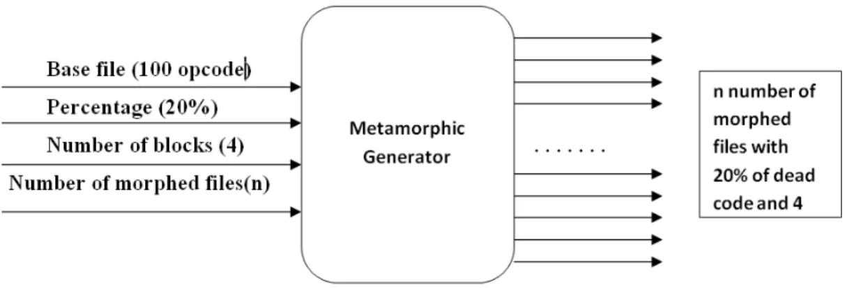
Figure 1: Metamorphic Generator

have chosen the dead code insertion technique for morphing. Ideally, the control and data flow of the code need to remain the same, and various jump statements can be used to achieve it. But, it would be easier to detect virus because of many jump statements. So, we did not try to maintain code execution sequence in same manner for morphed files, which eventually make harder case.

Initially, the program asks for morphing percentage and the number of blocks for dead code insertion. Suppose, that morphing percentage and number of blocks are given as 20 and 4 respectively, and we have a base file of 100 opcode. Then, the total number of opcode needed for dead code will be20and distributed5opcodes per block. Next, using random function of JAVA, it generates 4random numbers for the position of dead code insertion. The output file will become the size of 120 opcode. We can generate as many morphed files as required using metamorphic generator. Morphing percentage is one of the measures to check the robustness of our detection techniques. Here, we are simulating the way an attacker could have targeted any piece of software using dead code insertion.

(20)

Figure 2: Block Insertion

2.3 Techniques for Metamorphism

In the following section, we discuss some common techniques to generate the metamorphic code like dead code insertion, code permutation, insertion of jump in-struction, and instruction replacement.

2.3.1 Dead Code Insertion

Dead code insertion is one of the simplest methods of morphing used by a meta-morphic engine. In this method, a sequence of bytes is changed by inserting the dead code [23]. Ideally, instructions used for the dead code should not have any effect on the functionality of the original code [15]. Dead code is similar to a null operation [14]. The inserted dead code will never be executed, so it has no semantic effect on the software [4]. This strategy could be used to evade signature based detection and is succeeding against statistical based detection [3]. The example shown in Table 1, demonstrates the dead code insertion.

(21)

Table 1: Dead Code Insertion Original Code After Garbage Insertion ADD 1055h, EAX ADD 1055h, EAX

SUB EAX JMP loc1234

POP EBX PUSH EBX PUSH EBX POP EBX

loc1234 SUB EAX

In Table 1 we can see that, in the original code, execution of the ADD instruction is followed by SUB, whereas in the code after garbage insertion, ADD is followed by the JMP, which immediately transfers the control to the SUB. All the dead code between ADD and SUB is eliminated by JMP instruction and the dead code does not have any effect on the actual code execution.

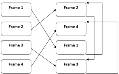
2.3.2 Code Permutation

In this method, code is divided into small modules (frames). After dividing the code, different modules are rearranged randomly by keeping the logic of the original code as it is. Various jump statements are used to maintain the logic of the code. Figure 3 illustrates the code permutation technique. So, this technique apparently changes the appearance of the software by reordering the frame sequences. If we have

𝑛 frames of the software, then 𝑛! unique generations are possible [5].

2.3.3 Insertion of Jump Instructions

JMP is assembly language instruction. It carries out an unconditional jump. It takes memory address, which are labeled in assembly language, as arguments [23].

(22)

Figure 3: Code Permutation

Figure 4: Insertion of Jump Instructions

JMP is used to change the address of targeted instruction. However, the flow of the program remains the same [23]. Many JMP are more prone to detections as it provides the identification.

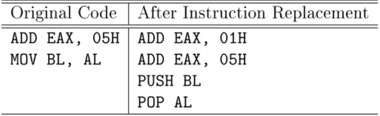
2.3.4 Instruction Replacement

In this method, instruction or a set of instructions is replaced by equivalent instruction or set of instructions. For example, different registers movements are

(23)

Table 2: Instruction Replacement Original Code After Instruction Replacement ADD EAX, 05H ADD EAX, 01H

MOV BL, AL ADD EAX, 05H

PUSH BL POP AL

replaced by number of PUSH and POP sequences. Instructions like OR-TEST and XOR-SUB can be used interchangeably [15]. Table 2 illustrates the instruction replacement techniques. Here, in the code after instruction replacement, ADD is replaced with two ADD instructions and MOV operation is performed using PUSH and POP operation. This technique defends strongly against the signature base detection.

2.4 Hidden Markov Model

A hidden Markov model (HMM) is a machine learning techniques [35]. As the name suggests, an HMM includes a Markov process and this process is the “hidden” part of the HMM. That is, the Markov process is not directly observable. But we do have indirect information about the Markov process via a series of observations that are probabilistically related to the underlying Markov process. The utility of HMMs derives largely from the fact that there are efficient algorithms for training and scoring. HMM have been used in various fields like malware detection [19] and speech recognition [25]. Following are the important notation to understand the Hidden Markov Model [35]:

(24)

𝑇 =length of the observation sequence

𝑁 =number of states in the model

𝑀 =number of observation symbols

𝑄={𝑞0, 𝑞1, . . . , 𝑞𝑁−1}=distinct states of the Markov process

𝑉 ={0,1, . . . , 𝑀 −1}=set of possible observations

𝐴=state transition probabilities

𝐵 =observation probability matrix

𝜋 =initial state distribution

𝒪 = (𝒪0,𝒪1, . . . ,𝒪𝑇−1) =observation sequence. Markov process: 𝑋0 - 𝑋1 𝑋2 · · · 𝑋𝑇−1 𝐴 -𝐴 -𝐴 -𝐴 ? 𝐵 ? 𝐵 ? 𝐵 ? 𝐵 Observations: 𝒪0 𝒪1 𝒪2 · · · 𝒪𝑇−1

Figure 5: Hidden Markov Model

Three matrices 𝐴, 𝐵 and 𝜋 are used to define hidden Markov model. HMM is

presented as 𝜆 = (𝐴, 𝐵, 𝜋). There are three basic problems that can be answered using hidden Markov model.

Problem 1: For a given model 𝜆= (𝐴, 𝐵, 𝜋)and a sequence of observations 𝒪, we

can determine 𝑃(𝑂|𝜆). That is, we can score an observation sequence to determine how well it fits a given model [35].

(25)

Problem 2: For a given model 𝜆 = (𝐴, 𝐵, 𝜋) and a sequence of observations 𝒪,

we can determine an optimal state sequence for the Markov model. That is, we can uncover the hidden part of the model [35].

Problem 3: For a given observation sequence 𝒪, and specific values of 𝑁 and 𝑀

we can determine a model. That is, we can train a model to fit a given observation sequence [35].

There are two main phases in HMM—Training and Detection. Training phase is to retrieve model that contains𝐴,𝐵, and 𝜋 matrices. This model will be used for

scoring files. 2.4.1 Training

In this phase, the opcode sequences are extracted from the base software. Using these opcode sequences, various slightly morphed copies of the base software are generated. These morphed copies are appended and finally hidden Markov model is trained on it. The reason for using slightly morphed copies is to avoid over fitting the training data for HMM [21]. At the end of the training phase, we retrieve 𝐴, 𝐵, and 𝜋.

2.4.2 Detection

In this phase, the opcode sequence from the suspected software is extracted. This sequence is scored against the trained HMM, which was derived in the previous phase. Then, score is compared against the previously calculated threshold value. The score above threshold indicates that further investigation is needed because suspected software is very similar to the base software. On the other hand, score below the

(26)

threshold signifies that suspected software is not similar to the base software. In our case, we mainly interested in separation between benign files and suspected files. Therefore, we did not bother about setting the threshold.

2.5 Opcode Graph Similarity

The paper [1] suggests one interesting graph based technique for malware detec-tion. The same technique can be used for the software similarity detecdetec-tion. Firstly, opcode sequence from the software is extracted to construct weighted directed graph. Each distinct opcode are assigned to the node in weighted directed graph. A directed edge is linked from a node to all the possible successor node. Weight of a particular edge gives the probability of corresponding successor node. The following example demonstrates the process. We used one dummy sequence of the opcodes as shown in the Table 3.

Using the Table 3, we obtained the counts for each digram of opcodes. These counts are shown in the Table 4. For example, the opcode SUB is immediately followed by the opcode JMP at 2 places (lines 10 and 20 in Table 3).

Using the digram frequency counts from Table 4, probability Table 5 is generated. Each cell in Table 5 represents a probability for occurrence of the given opcode after any opcode. Each entry in the Table 4 is divided by the sum of each entry of the corresponding row. The resulting probability table is shown in the Table 5. For example, JMP occurs 6 times in the table while (JMP, SUB) occurs 2 times. Therefore, (JMP, SUB) entry in the Table 5 contains the probability 1/3.

Using the entries from the Table 5 opcode directed graph is prepared. This directed probability graph is represented as adjacency matrix for ease of calculations.

(27)

Table 3: Opcode Sequence 1 CALL 2 JMP 3 ADD 4 SUB 5 NOP 6 CALL 7 ADD 8 JMP 9 JMP 10 SUB 11 JMP 12 ADD 13 NOP 14 JMP 15 CALL 16 CALL 17 CALL 18 ADD 19 JMP 20 SUB

Table 4: Opcode Count ADD CALL JMP NOP SUB

ADD 0 0 2 1 1

CALL 2 2 1 0 0

JMP 2 1 1 0 2

NOP 0 1 1 0 0

SUB 0 0 1 1 0

Table 5: Probability Table ADD CALL JMP NOP SUB

ADD 0/4 0/4 1/2 1/4 1/4

CALL 2/5 2/5 1/5 0/5 0/5

JMP 1/3 1/3 1/3 0/6 1/3

NOP 0/2 1/2 1/2 0/2 0/2

(28)

2.6 Simple Substitution Distance

Substitution cipher is one of the oldest cipher systems [36]. In this system, each plaintext symbol is substituted by ciphertext symbol. These symbols could be letters, digrams, or trigrams. There are many types of substitution ciphers. In the following section, we briefly discuss simple substitution ciphers.

2.6.1 Simple Substitution Ciphers

Simple Substitution ciphers are one of the simplest form of substitution ci-phers [36]. In this cipher, plaintext symbol maps to one ciphertext symbol [9, 18]. A simple substitution key is shown in Table 6. In that, each ciphertext letter is obtained by shifting the plaintext letter by 3 positions forward in the alphabetical order [36]. Hence, plaintext message HELLO is encrypted to KHOOR, if the key in Table 6 is used for encryption [3].

Table 6: Simple Substitution Key

plaintext: A B C D E F G H I J K L M N O P Q R S T U V W X Y Z ciphertext: D E F G H I J K L M N O P Q R S T U V W X Y Z A B C Simple substitution consists 26! possible keys if plaintext is in the English lan-guage. To break the system attacker needs to try 287 keys on average [9]. If the attacker has high computation power that can test 240 keys per second, then brute force attack will take around 247 seconds (millions of years) [9]. It is impractical to try such a huge key space. But attacker uses different approaches like English monograph statistic to crack the ciphertext [9]. For example, most frequent cipher-text letter maps to most frequent letter in the English cipher-text E, similarly second most frequent letter maps to second most frequent letter in the English text T, and so on. Using this technique, an attacker will be able to recover most of the plaintext very

(29)

fast. Then, he can guess for the remaining message [9]. 2.6.2 Fast Attack on Simple Substitution

An algorithm to crack the simple substitution cipher is mentioned in [12]. It initially guesses the key and modifies the key in each iteration by swapping elements in key. Correctness of key is determined by checking the closeness between digram matrix obtained from English plain text and decrypted text. The lower the score, the higher the correctness of the key. This algorithm is explained in section 2.6.4.

2.6.3 Solution Using Hill Climbing Problem

Hill climb is a mathematical optimized technique that starts with some initial solution and try to finds better solutions by doing minor changes to the putative solu-tion. The new score is compared against the previous score. If the score improves, the incremental changes are made [9]. This process is repeated until the better solution is obtained [9, 43].

2.6.4 Overview of Jackobsen’s Algorithm

Jackobsen’s algorithm [12] make assumptions about plaintext and ciphertext. It assumes that plaintext and ciphertext are in English and contains 26 alphabets. It makes an initial guess about key using frequency of letters that is most frequent letter in ciphertext maps to the most frequent letter in English text E, second most frequent letter maps to T, and so on.

In the subsequent iterations, algorithm modifies the current key and uses it to decrypt ciphertext. If putative plaintext is closer to the expected English text than before, the new key is used for next iterations; otherwise the old key is modified in a

(30)

different way. This process is repeated around (︀26 2

)︀

times, so that every elements of key are swapped at least once.

The scheme to modify the key is explained in [9]. Suppose that the putative key is 𝐾 = 𝑘1, 𝑘2, 𝑘3, 𝑘4, . . . , 𝑘25, 𝑘26. Here, 𝐾 is permutation of english letters. At beginning, the swapping takes place between adjacent elements. That is 𝑘1 with 𝑘2,

𝑘2 with 𝑘3 and so on. In the second iteration, elements away by two from each other are swapped, that is 𝑘1 with 𝑘3, 𝑘2 with 𝑘4 and so on. Same way in third iteration, elements away by three from each other are swapped. In the 𝑛𝑡ℎ iteration, elements away by 𝑛 from each other are swapped. The process is presented diagrammatically

in [9] which is shown in (1). round 1: 𝑘1|𝑘2 𝑘2|𝑘3 𝑘3|𝑘4 . . . 𝑘23|𝑘24 𝑘24|𝑘25 𝑘25|𝑘26 round 2: 𝑘1|𝑘3 𝑘2|𝑘4 𝑘3|𝑘5 . . . 𝑘23|𝑘25 𝑘24|𝑘26 round 3: 𝑘1|𝑘4 𝑘2|𝑘5 𝑘3|𝑘6 . . . 𝑘23|𝑘26 .. . ... . .. round 24: 𝑘1|𝑘24 𝑘2|𝑘25 𝑘3|𝑘26 round 25: 𝑘1|𝑘25 𝑘2|𝑘26 round 26: 𝑘1|𝑘26 (1)

where, ‘|’ means swap.

Using diagraph distribution matrix of putative key, the current key is modified [9]. This procedure is explained later in this section. To determine the closeness between digraph distribution matrix of putative plaintext and English language, the following scoring function (2) is used [9].

score(𝐾) = 𝑑(𝐷, 𝐸) =∑︁ 𝑖,𝑗

(31)

Table 7: Frequency Count E T A O I N S R H D 11 9 5 4 4 6 3 5 2 12

Table 8: Putative Key K

Plaintext: E T A O I N S R H D

Ciphertext: D E T N A R I O S H Where,

𝐷=𝑑𝑖𝑗 represents the putative plaintext digraph distribution matrix

𝐸 =𝑒𝑖𝑗 represents the expected English language digraph distribution matrix

𝐾 =similarity between two matrices (𝐾 is always greater than or equal to zero)

Procedure for modifying 𝐾 is explained in [9]. We also mentioned it below. If we

have simple substitution cipher that is based on English letters, descending order of plaintext symbols according to the frequency is

E, T, A, O, I, N, S, R, H, D M, O, P, S, J, R, U, Y, B, K

Suppose the ciphertext is [27]

TNDEODRHISOADDRTEDOAHENSINEOARDTTDTINDDRNEDNTTTDDISRETEEEEEAA The frequency count corresponding to the ciphertext is shown in Table 7 and the initial putative key 𝐾 is shown in Table 8. Putative plaintext will be [9]

(32)

Table 9: Diagraph Distribution Matrix E T A O I N S R H D E 3 1 2 1 0 3 1 1 0 0 T 2 4 1 1 1 0 0 2 0 0 A 2 2 2 1 0 0 1 0 0 0 O 2 2 1 0 0 0 0 0 1 0 I 1 0 0 0 1 1 0 0 0 1 N 1 1 1 1 0 0 0 0 0 1 S 0 0 0 2 0 0 0 0 2 0 R 1 0 0 0 3 0 0 0 0 0 H 0 0 0 0 0 1 1 1 0 0 D 0 1 0 0 0 0 1 0 0 0

Table 10: New Putative Key

Plaintext E T A O I N S R H D

Ciphertext E D T N A R I O S H

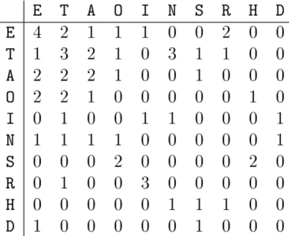
The digraph distribution matrix is shown in Table 9. Now, we will modify putative key as we discussed in swapping procedure. First, we swap the first two elements [9]. New putative key is shown in Table 10. Now, corresponding new putative plaintext will be [9]

AOTERTNDSHRITTNAETRIDEOHSOERINTAATASOTTNOETOAAATTSHNEAEEEEEII Diagraph distribution matrix of putative plaintext is shown in Table 11. From the matrix, we can see that, by swapping corresponding row and column we can swap the elements in key.

2.7 Singular Value Decomposition

Properly created metamorphic malware can avoid signature base detection, as well as other detection techniques based on statistical analysis [3]. On the other hand, some techniques based on compression rate, file entropy, and eigenvalue analysis seem to be more precious for malware detection [13]. We want to use such techniques for

(33)

Table 11: Corresponding Diagraph Distribution Matrix E T A O I N S R H D E 4 2 1 1 1 0 0 2 0 0 T 1 3 2 1 0 3 1 1 0 0 A 2 2 2 1 0 0 1 0 0 0 O 2 2 1 0 0 0 0 0 1 0 I 0 1 0 0 1 1 0 0 0 1 N 1 1 1 1 0 0 0 0 0 1 S 0 0 0 2 0 0 0 0 2 0 R 0 1 0 0 3 0 0 0 0 0 H 0 0 0 0 0 1 1 1 0 0 D 1 0 0 0 0 0 1 0 0 0 software piracy detection.

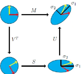
Eigenfaces, a technique for facial reorganization is the foundation for this imple-mentation [40]. Singular value decomposition [29] is factorization of the real matrix. The main idea behind the SVD is to consider the high variable dataset and reduce it to the lower dimension dataset in such a way that it clearly defines the substructure of the original dataset [13]. The SVD of the real matrix 𝐴 yields a factorization of

the form

𝐴=𝑈 𝑆𝑉𝑇.

Here, matrix 𝑈 is the left singular vector of matrix 𝐴. 𝑈 is calculated by the

eigenvectors of 𝐴𝐴𝑇. Also, matrix _𝑉 is the right singular vector of matrix _𝐴. _𝑉 is calculated by the eigenvectors of 𝐴𝑇_𝐴. Matrix _𝑆 is the diagonal matrix. It is calculated by taking the square root of eigenvalues, which is common to both the matrix 𝑈 and 𝑉. 𝑈 𝑈𝑇 and _𝑉𝑇_𝑉 are two identity matrices. The eigenvectors of the matrix 𝑈 is called singular vector because the eigenvector of the matrix 𝑈 are

normalized. Normalization is done by dividing every eigenvector by square root of corresponding eigenvalue. Matrix 𝑈 contains all eigenvectors as per the singular

(34)

Figure 6: SVD on Matrix A, Matrix Transformation values of the matrix 𝐴. SVD on matrix 𝐴 is shown in Figure 6 [13].

2.7.1 SVD Algorithm

SVD algorithm can be described in two phases. Training phase followed by testing phase. In the training phase, weights of the input files are determined by projecting them onto eigenspace. In the testing phase, suspected files and benign files are projected onto the eigenspace and their weights are determined. Finally, euclidean distance between the weights of training files and testing files are calculated. Step by step procedure of training phase and testing phase are described below.

2.7.1.1 Training Phase

First, we extract raw bytes from all the input files, and for each of these input files, we construct column vector. Then, the eigenvectors of the covariance matrix were determined. Eigenvectors with low eigenvalues are ignored as they are less important. Then, on eignespace, we project all the files to get weight. This phase is explained as below.

(35)

∙ Get 𝑀 number of files for training and extract raw bytes. Construct matrix 𝐴

using the vector of all files.

𝐴 = [𝜑1𝜑2𝜑3. . . 𝜑𝑀]. (3) Suppose,𝑁 is the maximum number of bytes an individual file contains, among

all files, then matrix𝐴will have𝑁 rows. Zeros are appended to column vectors,

which contains less than 𝑁 bytes. To identify variance between different files,

eigenvectors of covariance matrix 𝐶 is determined by 𝐶 = 1 𝑀 𝑀 ∑︁ 𝑖=1 𝜑𝑖𝜑𝑇𝑖 =𝐴𝐴𝑇 (4) In equation (4), 𝑀 is the number of files.

∙ Dimensions of matrix𝐴and𝐶are𝑁×𝑀 and𝑁×𝑁 accordingly. It is very hard

to find the eigenvectors of such a large matrix. So alternatively we can calculate eigenvectors for another matrix 𝐿 of dimension 𝑀 ×𝑀. 𝐿 is calculated using 𝐴𝑇_𝐴_{. In following equation (5)} _𝑣

𝑖 is the eigenvector of 𝐿 and it is calculated using

𝐿𝑣𝑖 =𝜆𝑖𝑣𝑖

𝐴𝑇𝐴𝑣𝑖 =𝜆𝑖𝑣𝑖

(5) Here,𝑣𝑖 is eigenvector and𝜆𝑖is eigenvalue. If we multiply the above equation (5) with 𝐴, it will give eigenvectors of matrix 𝐶

𝐴𝐴𝑇𝐴𝑣𝑖 =𝜆𝑖𝐴𝑣𝑖

𝐶𝐴𝑣𝑖 =𝜆𝑖𝐴𝑣𝑖

(6) where 𝐴𝑣𝑖 is the eigenvector of 𝐶. This is called reduce singular value decom-position. Now, according to the eigenvalues, sort the eigenvectors in descending order, because eigenvectors with higher eigenvalues are more important.

(36)

∙ We took 𝑀′ eigenvectors out of 𝑀, where 𝑀′ is less than 𝑀. We project

these eigenvectors into the space and space spanned by these vectors are called eigenspace. We can create original software replicate from𝑀′ vectors by adding

their corresponding weight. Suppose, for software file 𝑉 in the training set

having eigenvectors 𝑢𝑖, we can generate software file as

𝑉 =𝑤1 ×𝑢1+𝑤1×𝑢1+. . .+𝑤𝑀′ ×𝑢_𝑀′ 𝑉 = 𝑀′ ∑︁ 𝑖=1 𝑤𝑖𝑢𝑖 (7) Then we can get weight of each file as shown in equation (8) and we can represent set of weight as 𝑤𝑖 = 𝑀′ ∑︁ 𝑖=1 𝑢𝑇_𝑖 𝑉 (8) Ω𝑇_𝑖 = [𝑤𝑖, 𝑤2, 𝑤3, . . . , 𝑤𝑀′] (9)

∙ The weights of all software files together ∆is shown in equation (10). Weights of all the files together on eigenspace will be the output of the training phase.

∆ = [Ω1,Ω2,Ω3, . . .Ω𝑀] (10)

2.7.1.2 Testing Phase

In this phase, we project column vector of each test files on eigenspace. We append zeros to the file that has less than 𝑁 bytes and remove bytes from the file

that is more than 𝑁 bytes.

𝑤𝑖 = 𝑀′ ∑︁ 𝑖=0 𝑒𝑇_𝑖 𝑉𝑛 (11) Ω𝑇_𝑛 = [𝑤1, 𝑤2, 𝑤3, . . . , 𝑤𝑀′] (12)

Once we have weight for test files, we compare them with a weight vector of training files. Then, we can calculate euclidean distance between these vectors. IfΩ𝑖

(37)

is weight vector for training file then euclidean distance will be distance= √︁ (𝜔2 1 −𝑤21) + (𝜔22−𝑤22) +. . .+ (𝜔𝑀 ′ 1 −𝑤𝑀 ′ 1 ) (13)

where 𝜔 is weight of test file and 𝑤 is weight of training file.

2.8 Compression-Based Analysis

Utilizing structural entropy analysis is one of the novel approaches for software piracy detection. It has been already used against code obfuscation yielding positive results in [2, 34]. It uses the structural entropy to find variations within the files and calculate a similarity measure. This technique has two major phases: file seg-mentation followed by sequence comparison. The file segseg-mentation includes entropy measurement with wavelet analysis. Finally, similarity is measured using levenshtein distance.

2.8.1 Structural Entropy

Structural entropy was originally proposed in [34]. It has produced good results for polymorphic malware and metamorphic malware [2, 16]. Unlike other techniques, this technique will not work on opcode sequence; it works on raw byte of the file.

The proposed technique for detection of software piracy is an extension of the technique presented in [2, 16]. Our technique can be divided into two major parts: file segmentation and sequence comparison. File segmentation achieved using Shannon’s formula, where entropy is calculated. Once entropy is calculated, wavelet transform is applied [16]. Figure 7 gives the pictorial representation of segmentation process. For sequence comparison, edit distance algorithm is used [16]. Finally, using the similarity formula, the result of the algorithm is compared against the pre-defined threshold.

(38)

Figure 7: File Segmentation 2.8.2 Classification Based on Compression

Previous research [8] has been done using compression for malware detection. It is based on the principle: given two similar strings, they can be compressed more together than compressed separately. One unknown string is compared against sev-eral known strings. Each known string represents unique family. Unknown file is considered of the family with which it best matches [16]. The detection framework is described in the Algorithm 1 and is mentioned in [8].

Detection framework is highly successful. However, the drawback is, memory usage [8] increases rapidly as the size of software increases, which could be a problem in case of very big software.

One another technique based on compression is described in [45]. It depends on detection framework, which uses a learning engine for training on malware and benign code. Using this partial matching phenomenon, two compression models are created. One of these represents the malware code and other represent the benign code. For

(39)

Algorithm 1 Kolmogorov Complexity Based Detection Framework

1: Input : (1) Training set 𝑇 𝑅 = {𝑇 𝑅+, 𝑇 𝑅−}, where 𝑇 𝑅+ is set of malware instance, and 𝑇 𝑅− is set of benign code instances. (2) Test set , 𝑇 𝐸 =

{𝑇 𝐸1, . . . , 𝑇 𝐸𝑛}, where 𝑇 𝐸𝑖 is the 𝑖𝑡ℎ (𝑖= 1. . . 𝑛) code instance. (3) Estimating function for Kolmogorov complexity, denoted by 𝐾.

2: Output: Classification 𝐶𝐿(𝑇 𝐸𝑖)𝜖{+,−}, which corresponds to a benign or mal-ware instance. 3: 𝑀+←𝐾(𝑇 𝑅+); 4: 𝑀− ←𝐾(𝑇 𝑅−)); 5: for i=1 to n do 6: 𝑀1 𝑖 −𝐾(𝑇 𝐸𝑖∪𝑀+); 7: 𝐵𝑖𝑡𝑠(𝑇 𝐸𝑖, 𝑀+) =𝑠𝑖𝑧𝑒𝑜𝑓(𝑀𝑖1); 8: 𝑀2 𝑖 =𝐾(𝑇 𝐸𝑖∪𝑀−); 9: 𝐵𝑖𝑡𝑠(𝑇 𝐸𝑖, 𝑀−) =𝑠𝑖𝑧𝑒𝑜𝑓(𝑀𝑖2); 10: 𝐶𝐿(𝑇 𝐸𝑖) =𝑎𝑟𝑔𝑚𝑖𝑛𝑐𝜖{+,−}𝐵𝑖𝑡𝑠(𝑇 𝐸𝑖, 𝑀𝑐) 11: end for

Algorithm 2 PPM Based Classification

1: Input : Training set 𝑇 = 𝑇+∪𝑇−, test set 𝑃 = {𝑋1, . . . , 𝑋𝑛}, and the order of the Markov model in PPM,𝑘.

2: Output: Classification of 𝑐(𝑋𝑖)𝜖{+,−} of 𝑋𝑖𝜖𝑃, for 𝑖= 1, . . . , 𝑛. 3: 𝑀+←𝐶𝑟𝑒𝑎𝑡𝑒𝑃 𝑃 𝑀(𝑇+); 4: 𝑀−←𝐶𝑟𝑒𝑎𝑡𝑒𝑃 𝑃 𝑀(𝑇−); 5: for all 𝑋𝜖𝑃 do 6: 𝐵𝑖𝑡𝑠(𝑋, 𝑀+) =𝐶𝑜𝑚𝑝𝑢𝑡𝑒𝐵𝑖𝑡𝑠(𝑋, 𝑀+); 7: 𝐵𝑖𝑡𝑠(𝑋, 𝑀−) =𝐶𝑜𝑚𝑝𝑢𝑡𝑒𝐵𝑖𝑡𝑠(𝑋, 𝑀−); 8: 𝑐(𝑋) =𝑎𝑟𝑔𝑚𝑖𝑛𝑐𝜖{+,−}𝐵𝑖𝑡𝑠(𝑋, 𝑀𝑐); 9: end for

any suspected file, average numbers of bits are used to encode it using aforementioned compression model. The suspected file is then classified by the compression rate. Algorithm 2 describes this process.

(40)

CHAPTER 3 Implementation

In this section, we discuss about implementation of all techniques. We started with implementation of Hidden Markov Model, followed by Opcode Graph Similarity, Simple Substitution Distance, Singular Value Decomposition, and Compression Based Analysis.

3.1 Implementation of Hidden Markov Model

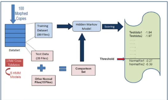
For training the Hidden Markov Model, we extracted opcode sequences from the base software. Then, we generated five 5% morphed copies of base software using metamorphic generator. All these five files were merged to obtain long observation sequences [20, 44].

Five-fold cross validation was used in this technique. It means, that we divided all files into five subsets. Four subsets were used for training the HMM and remaining one was used as test data [20]. This process is repeated five times; each time testing subset and training subset changes accordingly [20, 44]. Training and scoring phase of HMM is shown in Figure 8.

Secondly, we scored 100 files of each case, that is, 10% morphing to 400% mor-phing. Then, we scored benign files for comparison. Finally, we plotted ROC curve and AUC.

(41)

Figure 8: Training and Scoring Phase of HMM 3.2 Implementation of Opcode Graph Similarity

Our goal is to develop the similarity measure from the extracted opcode se-quences [26]. First, we extracted the opcode sequence and prepared the weighted directed graph. So far, our technique is similar to the technique used in [1]. But, instead of using graph kernels to generate scores, we directly compared the opcode graphs [26].

Let 𝑁 be the total number of the distinct opcode from the extracted opcode

sequences. We map this opcode to 0,1,2,3, . . . , 𝑁 −1. Let 𝐴 =𝑎𝑖𝑗 and 𝐵 =𝑏𝑖𝑗 be the two edge weighted matrices corresponding to the two executable files (in our case, base software and suspected software), same as Table 5. Note that, both𝐴and𝐵 are

of size 𝑁 ×𝑁 and both have the same opcode numbering [26]. It means, 𝑎𝑖𝑗 and 𝑏𝑖𝑗 represent the opcode 𝑖 is followed by opcode 𝑗 corresponds to 𝐴 and 𝐵 [26]. In case

of different number of distinct opcode in both opcode sequences, we take the superset of distinct opcodes from both sequences. Now, for comparing these matrices, we used

(42)

following equation. score(𝐴, 𝐵) = 1 𝑁2 (︃_𝑁₋₁ ∑︁ 𝑖,𝑗=0 |𝑎𝑖,𝑗−𝑏𝑖,𝑗| )︃2 (14) If 𝐴 and 𝐵 are equal, then minimum score 0is obtained. If 𝑎𝑖𝑗 = 1 and 𝑏𝑗𝑘 = 1, for 𝑗 ̸=𝑘, then maximum possible row sum

𝑁−1

∑︁

𝑗=0

|𝑎𝑖,𝑗−𝑏𝑖,𝑗|= 2 (15)

is obtained [26]. Maximum possible score of 4 is achieved if maximum row sum is achieved for all rows and hence, 0≤score(𝐴, 𝐵)≤4.

3.3 Implementation of Simple Substitution Distance

For software piracy detection, we used hill climb technique analogous to Jack-obsen’s algorithm [12]. The basic idea is that we train the detection system on a sequence of opcodes extracted from a five 5% morphed files and the trained system will be used to score suspected software to determine whether it is pirated or not. In the remainder of this section, we discuss the design of this technique in detail.

We extracted the opcode sequence from suspected software and base software. Using base software we created five 5% morphed files for training. Then, we con-structed two digraph distribution matrices, one using suspected file and other using training files. We mapped opcodes to indices 0,1,2,3, . . . , 𝑛−1. Any opcode other than the top n that occurs in the suspected files or the benign files are grouped to-gether under the same opcode category “Unknown”. Let 𝐷 = 𝑑𝑖𝑗 and 𝐸 = 𝑒𝑖𝑗 be the two digraph distribution matrices of suspected file and training files respectively. The size of both the matrices will be (𝑛+ 1×𝑛+ 1). Both 𝑑𝑖𝑗 and 𝑒𝑖𝑗 represent the probability of opcode 𝑖 followed by opcode 𝑗 in the suspected file and training files.

(43)

opcode in the training files. For the experiment, we considered five copies of slightly morphed base software. We assume that most frequent opcode in the training files maps to the most frequent opcode in suspected software, also the second most fre-quent opcode in training files maps to the second most frefre-quent opcode of suspected software, and so on. We created the 𝐷 matrix using initial key 𝐾, then normalized

it by dividing each cell with sum of all cells in matrix.

For constructing𝐸 matrix, suppose𝑚 denotes number of slightly morphed base

files. Then, we can construct𝑚matrices of size(𝑛+1)×(𝑛+1). We create matrix𝐹(0) with diagraph frequency counts of opcode in training file 0, and 𝐹(1) with diagraph frequency counts of opcode in training file1and so on. We normalized all the matrices by same way we normalized 𝐷matrix [9]. We created 𝐸 matrix as:

𝐸 ={𝑒𝑖,𝑗}=

(︁

𝐹_𝑖,𝑗(0)+𝐹_𝑖,𝑗(1)+. . .+𝐹_𝑖,𝑗(𝑚−1))︁/𝑚 (16)

Finally, to compare 𝐷 and 𝐸, we used following equation:

score(𝑘) =𝑑(𝐷, 𝐸) = ∑︁ 𝑖,𝑗

|𝑑𝑖,𝑗−𝑒𝑖,𝑗| (17) In the iterated loop, by swapping the opcode in the key

𝐾 =opcode₀,opcode₁,opcode₂,opcode₃, . . . ,opcode_𝑛₋₁,opcode_unknown

we changed the putative key, and the swapping is done the same way as in Jackobsen’s method [12]. In first iteration, all the opcode away from a distance of one are swapped, that is opcode0 with opcode1 and so on. In the second iteration, all the opcode away from a distance of two are swapped, that is, opcode0 with opcode2, and so on. Finally, in the 𝑛𝑡ℎ iteration, all the opcode away from distance of 𝑛 are swapped, that is,

opcode0 with opcode𝑛. After each swapping, we computed the score by comparing

(44)

again from the first iteration [9]. If the score does not improve, then we do other modification with the old key. We continue swapping for (︀𝑛

2

)︀

iterations to ensure all

(︀𝑛

2

)︀

pairs of opcodes in key are swapped at least once [9, 27]. Finally, we scored, 100 files of each cases, that is 10% morphing to 400% morphing and plotted ROC curve and AUC.

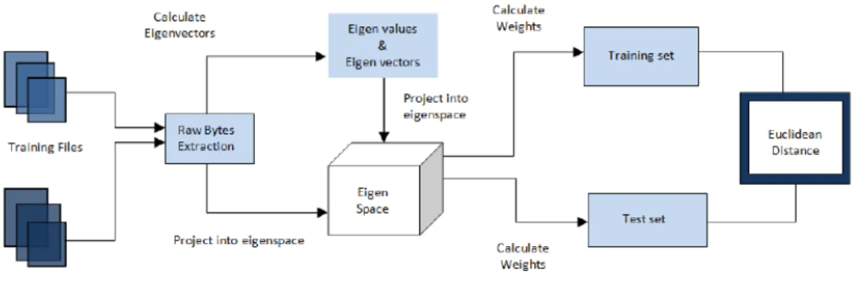
3.4 Implementation of Singular Value Decomposition

We extracted raw bytes from the text section of training files and constructed a training input matrix 𝐴. If we have 𝑀 files for training and Maximum number of

bytes among all files is 𝑁 then matrix 𝐴 will be of size 𝑁 ×𝑀. Zeros are append

to the files, which has fewer bytes than 𝑁 and first 𝑁 bytes are taken from the files

that have more than𝑁 bytes.

This matrix is passed to the JAMA API (JAVA Matrix Package), which is devel-oped in JAVA for the calculation of singular vectors and singular values. Using these singular vectors, we have calculated the weights of training files [13]. Weights for the testing files are calculated by projecting their column vectors on singular space. Once we have the weights for both training set files and testing set files, we can mea-sure the euclidean distance between the calculated weights. Figure 9 is the graphical representation of the process.

3.5 Implementation of Compression-Based Analysis

Implementation of compression based analysis has two major phases, File Seg-mentation followed by Sequence Comparison. File SegSeg-mentation phase measures the data complexity throughout the file using structural entropy and Sequence Compar-ison measures the similarity between files.

(45)

Figure 9: Process of Singular Value Decomposition

Figure 10: Sample File and It’s Hexdump 3.5.1 Creating File Segments

In this section we discuss about splitting the files into windows and then cal-culating the compression ratio for each window. Finally, wavelet transformation is applied in order to get smoothed data.

3.5.1.1 Splitting Files Into Byte Windows

First of all, this technique splits file into byte windows. These windows are strings of consecutive bytes, nearly the same size in terms of bytes. As we are considering file as a single stream of data, we should overlap windows to some extent. Window size and its slide size are determined experimentally [16]. As shown in the hex dump of sample file in Figure 10 [16], the file contains 103 bytes.

For example, the window size is 10 bytes and windows slide size is5 bytes. The first window is shown in Figure 11 and the second window is shown is Figure 12.

(46)

Figure 11: Sample File and It’s Windows1

Figure 12: Sample File and It’s Windows2

All the remaining windows are measured the same way. If the final window contains fewer bytes than the window size, null byte are appended [16].

In reality the windows size should be larger to derive any meaningful information from compression analysis. On the other hand, size should not be too large that it could allow attackers to mask any malicious code.

3.5.1.2 Compression Ratios for Windows

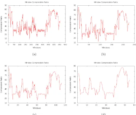
Having numbers of window, we need to calculate their compression ratio. The vi-tal part is that, windows with low entropy data should have higher compression ratio and windows with high entropy data should have lower compression ratio. There-fore, without having actual code, compression ratio gives us information about the underlying part of the file.

To calculate compression ratios, we used the software application named gzip. The main algorithm behind the gzip is lempel-ziv (LZ77) [16]. This algorithm mea-sures the distribution of unique byte sequence in the window. Figure 13 show, the compression ratio derived from an example file.

(47)

Figure 13: Window Compression Ratio of Sample File 3.5.1.3 Wavelet Transform Analysis

In the Figure 13, we can see that data can vary rapidly and it would be very hard to compare sets of plot. Using wavelet transformation, data can be smoothed where highly variations occur. In our implementation, we choose discrete Haar wavelet transform [16] from various wavelet transforms. We decided to choose it from previous work [2, 34]. This transforms gives simple and efficient results. Suppose, we have 𝑁

values: 𝑥= (𝑥1, 𝑥2, . . . , 𝑥𝑁). Here, 𝑁 is even number. 𝑠𝑘 and 𝑑𝑘 will be determined as 𝑠𝑘= 𝑥2𝑘−1+𝑥2𝑘 2 (18) and 𝑑𝑘 = 𝑥2𝑘−𝑥2𝑘−1 2 (19)

respectively. Discrete Haar wavelet transform can then be determined by [10]

(48)

Figure 14: Wavelet Transform for 0 Iteration, 1 Iteration, 2 Iteration and 3 Iteration Respectively

The 𝑠𝑘 contains set of values, known as pair-wise averages. We can perform discrete haar wavelet transform recursively and arbitrary times of iteration. The transform can only be applicable to sets, which contains even values. For the set, which contains an odd value, we need to pad last value to pretend as original data. Figure 14 shows the effect of three iterations on data.

3.5.1.4 Creation of File Segment

Next, we want to form the file segments. For that, we need threshold, which determine that which is high entropy and which is a low entropy [16]. In our experi-ment, we decided0.65as a threshold after examining calibration experiment [16]. So, values of compression ratio greater than 0.65considered low entropy and values less than 0.65are considered high entropy [16].

(49)

Table 12: Final File Segments

Segment # Segment Length Segment Value

1 1 0.820

2 1 0.640

3 3 0.897

4 2 0.575

5 3 0.903

Now, every segment has a length and value associated with it. Segment length represents all the values of compression ratio, contributing to a particular segment. The mean of all associated ratios are considered as the segment value. For example, suppose the final wavelet transformed values are 0.82, 0.64, 0.79, 0.90, 1.00, 0.60, 0.55, 0.93, 0.88, 0.90. Considering threshold of 0.65, Table 12 shows the resulting segment.

3.5.2 Comparison Between Sequences

The final sequence of segments represents a particular file. Now, the problem of file similarity becomes the problem of sequence comparison. For comparison, we used the levenshtein distance based algorithm. Finally, to determine the similarity we used the distance between the sequences. This approach is derived from [2, 34]. 3.5.2.1 Levenshtein Distance

To measure the difference between two files, a string metric named levenshtein distance is used [42]. It is also called the edit distance. Specifically, the levenshtein distance is the number of operations that need to be performed like insertion, deletion and substitution to convert𝑎into𝑏[6]. Lesser the operation, the more similar strings

are. For demonstration, we took two string abcde and azbcy. Assume the cost of each operation, insertion, deletion and substitution as 1. Then, to convert abcde to

(50)

azbcy,

abcde → azbcde (insert z)

azbcde → azbcye (substitute d for y)

azbcye → azbcy (delete e)

Since three operations are the minimum number of edits required to convert abcde to azbcy, the Levenshtein distance between these two strings is considered as three. Various combinations of operation is possible.

To generalize the process, if two sequences are 𝑋 = (𝑥1, 𝑥2, . . . , 𝑥𝑛) and 𝑌 = (𝑦1, 𝑦2, . . . , 𝑦𝑚), and cost of the functions are predefined than we can obtain the matrix of elements. Using the following recursion (21) elements of the matrix

𝐷(𝑛+1)×(𝑚+1) ={𝑑𝑖,𝑗} are computed as [2] 𝑑𝑖,𝑗 = ⎧ ⎪ ⎪ ⎪ ⎪ ⎪ ⎪ ⎪ ⎪ ⎨ ⎪ ⎪ ⎪ ⎪ ⎪ ⎪ ⎪ ⎪ ⎩ 0 if 𝑖=𝑗 = 0 𝑑0,𝑗−1+𝛿𝑦(𝑗) if 𝑖= 0 and 𝑗 >0 𝑑𝑖−1,0+𝛿𝑥(𝑖) if 𝑖 >0 and 𝑗 = 0 𝑑𝑖−1,𝑗−1 if 𝑥𝑖 =𝑦𝑗 min ⎧ ⎨ ⎩ 𝑑𝑖,𝑗−1+𝛿𝑦(𝑗) 𝑑𝑖−1,𝑗+𝛿𝑥(𝑖) 𝑑𝑖−1,𝑗−1+𝛿𝑋,𝑌(𝑖, 𝑗)) if 𝑥𝑖 ̸=𝑦𝑖 (21) Here, 𝛿𝑌(𝑗) =cost of insertion 𝛿𝑋(𝑖) =cost of deletion 𝛿𝑋,𝑌(𝑖, 𝑗) =cost of substitution

Considering the cost of 𝛿𝑌,𝛿𝑌 and 𝛿𝑋,𝑌 as 1 and using it with equation (21) for calculating the levenshtein distance for abcde and azbcy example, we get the matrix as shown in Table 13. The 𝑑𝑛,𝑚 gives the final score of the distance.

(51)

Table 13: Edit Matrix for Both Strings a b c d e 0 1 2 3 4 5 a 1 0 1 2 3 4 z 2 1 1 2 3 4 b 3 2 1 1 2 3 c 4 3 2 1 2 3 y 5 4 3 2 2 3 3.5.2.2 Sequence Alignment

Suppose we have 𝑋 and𝑌, two different files for similarity calculation. Then we

derived respective segment 𝑥𝑖 for 𝑖= 1,2,3, . . . , 𝑛and 𝑦𝑖 for 𝑗 = 1,2,3, . . . , 𝑚 as per the segmentation process. We used the cost function mentioned in [2, 34] to account for size differences.

cost𝜎(𝑥𝑖, 𝑦𝑗) =

|𝜎(𝑥𝑖)−𝜎(𝑦𝑗)|

𝜎(𝑥𝑖) +𝜎(𝑦𝑗)

(22) Here, 𝛿𝑌(𝑗) is size of segment 𝑥𝑖 and 𝛿𝑋(𝑖) is size of segment 𝑦𝑗.

The possible range of cost function is between0and 1inclusively. We use follow-ing cost function mentioned in [2, 34] with respect to compression ratio differences.

cost𝜖(𝑥𝑖, 𝑦𝑗) =

1

1 +𝑒−4|𝜖(𝑥𝑖)−𝜖(𝑦𝑗)+6.5| −0.001501 (23)

Here, 𝜖(𝑥𝑖)and 𝜖(𝑦𝑗)= compression ratios of respective segments. Two constant 6.5 and 0.001501 helps to produce the value of 𝑐𝑜𝑠𝑡𝜖 between 0 and 1 [2]. Using equations (22) and (23), the final version of the cost function is

cost(𝑥𝑖, 𝑦𝑗) =𝑐𝜎 cost𝜎(𝑥𝑖, 𝑦𝑗) +𝑐𝜖 cost𝜖(𝑥𝑖, 𝑦𝑗) (24) Here, 𝑐𝜎 is constant for size and 𝑐𝜖 is constant for entropy cost.

The cost function (24) applies to sequence alignment algorithm, which is based on levenshtein distance. Using dynamic programming, two-dimensional array similar

(52)

to Table 13 is created. Finally, got the last element for cost calculation between two-segment sequences [16]. To use, equation (21) for calculating elements of the array, we make 𝜏 = 0.3and prepared functions

𝛿𝑌(𝑗) =𝜏 log 𝜎(𝑦𝑗−1) 𝛿𝑋(𝑖) =𝜏 log 𝜎(𝑥𝑖−1) 𝛿𝑋,𝑌(𝑖, 𝑗) =cost(𝑥𝑖−1, 𝑦𝑗−1) log (︂ 𝜎(𝑥𝑖−1) +𝜎(𝑦𝑗−1) 2 )︂ (25)

The functions in (25) are derived in [2] 3.5.2.3 Similarity Calculation

Once we have calculated edit distance using equation (21) with penalty func-tions (25), we can calculate similarity between file 𝑋 and 𝑌 using [16]

similarity= 100 (︂ 1− 𝑑𝑛,𝑚 costmax )︂ (26) Here, costmax is worst case penalty and it is calculated in a special way as follow by considering penalty functions (28).

costmax=𝑑′0,𝑚+𝑑 ′ 𝑛,0 (27) 𝛿_𝑌′ (𝑗) = 𝛿𝑌(𝑗) 𝛿_𝑋′ (𝑖) = 𝛿𝑋(𝑖) 𝛿_𝑋,𝑌′ (𝑖, 𝑗) = 2𝜏(log 𝜎(𝑥𝑖−1) + log 𝜎(𝑦𝑗−1)) (28)

(53)

CHAPTER 4 Experimental Results

In all of the techniques we experimented, our main goal is to verify that, whether our techniques are able to distinguish between pirated software and legitimate soft-ware. We experimented with 10% of morphed files to 400% of morphed files. For each technique, we tried to find the point (morphing percentage) where techniques stop giving the ideal results. Finally, we plotted receiver operating characteristic curve (ROC) and area under the curve (AUC) for each case. We used cygwin utilities files as benign files and generated morphed copies using the metamorphic generator. 4.1 Hidden Markov Model

In our experiment, we found that up to 70% of morphing HMM is able to distin-guish between pirated software and legitimate software. From 80% onwards, technique is not able to distinguish properly. It happens because, as we add more deadcode, morphed files become more similar to the benign files and less similar to the original base software. We can clearly observe this in Table 14 of the AUC.

4.2 Opcode Graph Similarity

In our experiment, we found that up to 80% of morphing this technique is able to distinguish clearly between pirated software and legitimate software. This means that AUC remains 1 till 80% of morphing. For 90% and 100% of morphing AUC remains in the range of 0.9, which shows that this technique is able to distinguish until 100% of morphing. From the 300% onwards the technique is failing totally. It happens because, as we added more number of deadcode, morphed files start losing

(54)

Table 14: AUC - Hidden Markov Model Morphing Percentage(%) AUC

10 0.80937 20 0.745 30 0.71937 40 0.62313 50 0.6125 60 0.51562 70 0.51 80 0.51 90 0.3575 100 0.38813 200 0.20313 300 0.15188 400 0.1325

Figure 15: Hidden Markov Model AUC Plot

its originality from base software. We can clearly observe this in Table 15 for the AUC.

(55)

Table 15: AUC - Opcode Graph Similarity Morphing Percentage (%) AUC

10 1 20 1 30 1 40 1 50 1 60 1 70 1 80 1 90 0.96562 100 0.90250 200 0.17625 300 0 400 0

Figure 16: Opcode Graph Similarity AUC Plot 4.3 Simple Substitution Distance

In our experiment, we found that up to 100% of morphing this technique is able to clearly distinguish between pirated software and legitimate software. This means

(56)

Table 16: AUC - Simple Substitution Distance Morphing Percentage (%) AUC

10 1 20 1 30 1 40 1 50 1 60 1 70 1 80 1 90 1 100 1 200 0.996 300 0.896 400 0.856

that AUC remains 1 until 100% of morphing. From 200% to 400% morphing AUC remains in the range of0.9-0.8, which shows that the technique is able to distinguish up to that range. So, in our experiment up to 400% of morphing, which is the highest percentage of morphing we experimented with, the technique is not failing completely. We can clearly observe this in Table 16 for the AUC.

4.4 Singular Value Decomposition

In our experiment, we found that up to 50% of morphing, this technique is able clearly to distinguish between pirated software and legitimate software. This means that the AUC remains 1 until the 50% of morphing. From 60% to 400% morphing AUC remains in the range of 0.99 - 0.91, which shows that this technique is still able to distinguish in that range with clarity. So, in our experiment up to 400% of morphing, which is the highest percentage of morphing we experimented with, the technique is giving good results. We can clearly observe this in Table 17 for the AUC.

(57)

Figure 17: Simple Substitution Distance AUC Plot

(58)

Table 17: AUC - Singular Value Decomposition Morphing Percentage (%) AUC

10 1 20 1 30 1 40 1 50 1 60 0.99999 70 0.99769 80 0.98834 90 0.97959 100 0.97665 200 0.96776 300 0.95406 400 0.91427 4.5 Compression-Based Analysis

In our experiment, we found that up to 90% of morphing this technique is able to clearly distinguish between pirated software and legitimate software. This means that AUC remains 1 until 90% of morphing. From 100% to 400% morphing AUC remains in the range of0.9-0.8, which shows that the technique is able to distinguish up to that range. So, in our experiment up to 400% of morphing, which is the highest percentage of morphing we experimented with, the technique is not failing completely. We can clearly observe this in Table 18 for the AUC.

(59)

Figure 19: Compression-Based Analysis AUC Plot

Table 18: AUC - Compression-Based Analysis Morphing Percentage (%) AUC

10 1 20 1 30 1 40 1 50 1 60 1 70 1 80 1 90 1 100 0.97823 200 0.84218 300 0.83129 400 0.80136

(60)

CHAPTER 5

Conclusion and Future Work

All the techniques we discussed in the paper were previously used to detect metamorphic malware. In this paper, we proposed these techniques for the completely different approach of software piracy detection. We wrote our own metamorphic generator to replicate suspected software. Input to the metamorphic generator are numbers of the suspected software and amount of morphing percentage, and it will replicate suspected software accordingly. We used cygwin utilities files as benign files. First three techniques that are based on statistical analysis work on the disassembled files whereas last two techniques work directly on raw bytes of the file.

Our experimental results show that all the techniques are robust in detecting pirated software. The Hidden Markov Model is able to distinguish between pirated software and legitimate software up to 70% of morphing. The AUC for HMM falls gradually with morphing percentage. The opcode graph similarity method is able to distinguish up to 100% of morphing, Up to 80% it is distinguishing with 0% false positive and 0% false negative, which means AUC is 1 up to 80% . Over 100% of morphing AUC falls exponentially. Simple substitution distance is able to distinguish clearly up to 100% of morphing, that is with 0% false positive and 0% false negative. In singular value decomposition AUC is 1 up to 50% and in the range of 0.9 from 60% onward. Lastly, in Compression-based analysis AUC is 1 up to 100% and start falling from 200% onward.

For future work, one can try other morphing techniques than dead code insertion, like code permutation and instruction replacement. Morphing using the instruction

(61)

replacement technique could be hard to detect because instead of changing the code sequence or inserting some dead code, it actually changes the code. In addition, one can experiment with different types of files. Throughout our project, we experimented with executable files (.exe files), but one can experiment with other types like byte code. Various new metamorphic malware are coming into the market daily, so by observing them one can generate some challenging suspected software to experiment with.

This project can be extended by combining both static and dynamic birthmarks. All the techniques we experimented with are considered as static birthmark as they work on statistically available information. In contrast, dynamic birthmark work on information gathered by executing the program.

Finally, the results of all the techniques, we experimented with can be improved for a higher amount of morphing.

(62)

LIST OF REFERENCES

[1] Anderson, B.: Graph-Based Malware Detection Using Dynamic Analysis. Jour-nal in Computer Virology, 7(4) 247–258 (2011).

[2] Baysa, D., Low, R.M., Stamp, M.: Entropy And Metamorphic Malware. Journal of Computer Virology and Hacking Techniques, 9(4) 179–192 (2013).

[3] Borello, J., Me, L.: Code Obfuscation Techniques For Metamorphic Viruses. Journal in Computer Virology, 4(3) 30–40 (2008).

[4] Cesare, S.: Fast Automated Unpacking And Classification Of Malware. Masters Thesis, Central Queensland University. Retrieved from http://acquire.cqu. edu.au:8080/vital/access/manager/Repository/cqu:7351

[5] Computer Virus Creation kit. Retrived from http://www.informit.com/ articles/article.aspx?p=366890&seqNum=6

[6] Cormode, G., Muthukrishnan, S.: The String Edit Distance Matching Prob-lem With Moves. Journal in Association for Computing Machinery Transac-tions on Algorithms, 3(2) (2007). Retrieved from http://dimacs.rutgers.edu/ ~graham/pubs/papers/editmoves.pdf

[7] Costello, F., Bleakley, C., Aliefendic, S.: Using Whitespace Patterns To De-tect Plagiarism In Program Code. Retrieved from http://www.csi.ucd.ie/ content/using-whitespace-patterns-detect-plagiarism-program-code [8] Deng, W., et al: A Malware Detection Framework Based On Kolmogorov

Complexity. Journal of Computational Information Systems, 7(8) 2687–2694 (2011). Retrieved from http://www.jofcis.com/publishedpapers/2011_7_8_ 2687_2694.pdf

[9] Dhavare, A., Low, R., Stamp, M.: Efficient Cryptanalysis Of Homophonic Sub-stitution Ciphers. Cryptologia, 37(3) 250–281 (2013).

[10] Fleet, P.: The Discrete Haar Wavelet Transformation. Joint Mathematical Meet-ings, (2007). Retrieved from http://cam.mathlab.stthomas.edu/wavelets/ pdffiles/NewOrleans07/HaarTransform.pdf

[11] Gao, X., Stamp, M.: Metamorphic Software For Buffer Overflow Mitiga-tion. In Proceedings of the 2005 Conference on Computer Science and its Ap-plications, Retrieved from http://www.cs.sjsu.edu/faculty/stamp/papers/ BufferOverflow.doc