The autoregressive stochastic block model with changes in structure

The autoregressive

stochastic block model

with changes in structure

Matthew Ludkin, M.Sci.(Hons.), M.Res

Submitted for the degree of Doctor of

Philosophy at Lancaster University.

I declare that the work in this thesis has been done by myself and has not been submitted elsewhere for the award of any other degree.

Matthew Robert Ludkin

A version of Chapter 3 has been published as:

Ludkin, M., Eckley, I., and Neal, P. (2017). Dynamic stochastic block models: parameter estimation and detection of changes in community structure. Statistics

Acknowledgements

Network science has been a growing subject for the last three decades, with sta-tistical analysis of networks seing an explosion since the advent of online social networks. An important model within network analysis is the stochastic block model, which aims to partition the set of nodes of a network into groups which behave in a similar way. This thesis proposes Bayesian inference methods for problems related to the stochastic block model for network data. The presented research is formed of three parts. Firstly, two Markov chain Monte Carlo samplers are proposed to sample from the posterior distribution of the number of blocks, block memberships and edge-state parameters in the stochastic block model. These allow for non-binary and non-conjugate edge models, something not considered in the literature.

Secondly, a dynamic extension to the stochastic block model is presented which includes autoregressive terms. This novel approach to dynamic network models allows the present state of an edge to influence future states, and is therefore named the autoregresssive stochastic block model. Furthermore, an algorithm to perform inference on changes in block membership is given. This problem has gained some attention in the literature, but not with autoregressive features to the edge-state distribution as presented in this thesis.

Declaration ii

Acknowledgements iii

Abstract iv

List of Figures viii

List of Tables xi

1. Introduction 1

1.1. Modelling networks . . . 2

1.1.1. Notation and definitions . . . 3

1.1.2. Mathematical models for networks . . . 4

1.1.3. Statistical network models . . . 7

1.1.4. The stochastic block model . . . 12

1.2. Dynamic stochastic block models . . . 16

1.3. Contributions . . . 19

2. Arbitrary edge-states and unknown number of blocks in the stochastic block model 24 2.1. Introduction . . . 24

2.2. Model . . . 28

2.2.1. Prior for block structure . . . 31

2.4. Split-merge sampler . . . 36

2.5. Simulated data . . . 48

2.5.1. Example networks . . . 48

2.5.2. Assessing convergence . . . 56

2.6. Real data . . . 57

2.6.1. Macaque . . . 57

2.6.2. Enron . . . 61

2.6.3. Stack Overflow . . . 63

2.7. Concluding remarks . . . 64

3. Autoregressive stochastic block model with changes in block member-ship 67 3.1. Introduction . . . 67

3.2. The autoregressive stochastic block model . . . 71

3.2.1. Model . . . 71

3.2.2. Posterior distribution . . . 73

3.2.3. Identifiability . . . 76

3.3. Reversible jump MCMC . . . 78

3.3.1. Sampling scheme . . . 78

3.3.2. Updating change points and augmented edge states . . . 80

3.4. Initialisation of sampler state . . . 84

3.5. Simulation study . . . 87

3.6. Application: Communities of mice . . . 90

3.7. Concluding remarks . . . 94

4. Online monitoring of block membership in the autoregressive stochas-tic block model 98 4.1. Introduction . . . 99

4.3. SMC . . . 106

4.3.1. Sufficient statistics . . . 107

4.3.2. SMC algorithm . . . 111

4.4. Simulated data . . . 116

4.4.1. Comparison to offline methods . . . 120

4.5. Application to dynamic contact network . . . 123

4.5.1. Mice network . . . 123

4.6. Closing remarks . . . 126

5. Perspectives and future directions 129 A. Appendix for arbitrary edge-states and unknown number of blocks in the stochastic block model 133 A.1. Enron . . . 133

B. Appendix for autoregressive stochastic block model with changes in block membership 136 C. Appendix for monitoring block membership in the autoregressive stochas-tic block model 144 C.1. Posterior plots . . . 144

C.2. Trace of block membership per mouse . . . 148

List of Figures

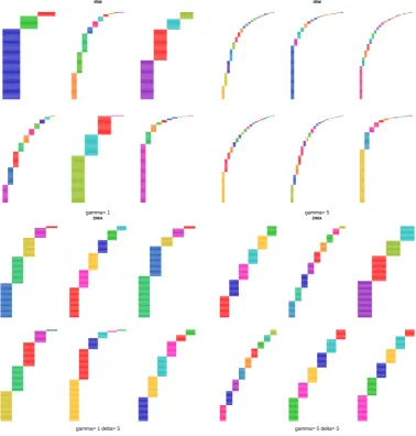
2.1. Comparison of block structures. Top left CRP(1), top right CRP(5). Bottom left: DMA(1,5), bottom right: DMA(5,5). . . 34 2.2. Posterior summaries for block membership in Bernoulli example

network. . . 52 2.3. Posterior summaries for block membership in Poisson example

net-work. . . 53 2.4. Posterior summaries for block membership in normal example

net-work. . . 54 2.5. Posterior summaries for block membership in negative binomial

ex-ample network. . . 55 2.6. Trace plots for number of blocks in example networks. Two chains

are simulated in each case: The “lower chain” with all nodes initially in one block (orange line) and the “upper chain” with all nodes initially assigned to different blocks (blue line). . . 58 2.7. Posterior summaries for block membership in Macaque brain

net-work using Dirichlet process sampler. . . 59 2.8. Posterior summaries for block membership in Macaque brain

net-work using Dirichlet process sampler. . . 60 2.9. Posterior summaries for block membership in Enron network with

Poisson edge-state model. . . 62 2.10. Posterior summaries for block membership in Enron network with

2.11. Posterior summaries for block membership in Stack Overflow network. 64

3.1. Possible changes. . . 81 3.2. Elbow plot for determining the number of communities with which

to initialise the sampler. . . 92 3.3. ARSBM: Maximum a posteriori community membership of each

mouse through time. Community labels: 1 red, 2 yellow, 3 -green, 4 - sky blue, 5 - dark blue, 6 - purple. . . 95 3.4. dynSBM: Maximum a posteriori community membership of each

mouse through time. Community labels: 1 red, 2 yellow, 3 -green, 4 - sky blue, 5 - dark blue, 6 - purple. . . 96

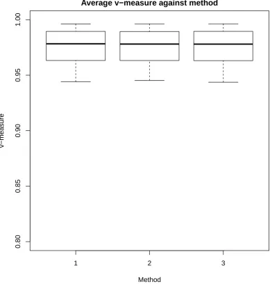
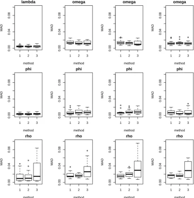
4.1. v-measure for simulated networks against method. 1 - Gibbs from mean, 2 - Gibbs from previous particle, 3 - store augmented states. 118 4.2. Mean absolute deviation for simulated networks against method.

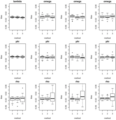
1 - Gibbs from mean, 2 - Gibbs from previous particle, 3 - store augmented states. . . 119 4.3. Bias for simulated networks against method. 1 - Gibbs from mean,

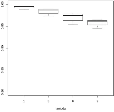
2 - Gibbs from previous particle, 3 - store augmented states. . . 120 4.4. v-measure against true λ values with method 2. . . 121 4.5. Comparison of v-measure for simulated networks under SMC and

RJMCMC algorithms. . . 124 4.6. Comparison of bias in parameters under SMC (left) and RJMCMC

(right) for example networks. . . 125 4.7. Maximum a posteriori block memberships of mice. . . 127

A.1. Posterior summaries for block membership in Enron network with Poisson edge-state model and strong prior. . . 134 A.2. Posterior summaries for block membership in Enron network with

B.1. Posterior density for each mouse’s community membership against

time. Shading implies levels of probability: White=0, Red=1 . . . . 137

B.2. Posterior density for each mouse’s community membership against time. Shading implies levels of probability: White=0, Red=1 . . . . 138

B.3. Posterior density for each mouse’s community membership against time. Shading implies levels of probability: White=0, Red=1 . . . . 139

B.4. Posterior density for each mouse’s community membership against time. Shading implies levels of probability: White=0, Red=1 . . . . 140

B.5. Posterior density for each mouse’s community membership against time. Shading implies levels of probability: White=0, Red=1 . . . . 141

B.6. Trace plots forπ and ρ parameters for mice data set. . . 142

B.7. Trace plots forλ and number of change-points for mice data set. . . 143

C.1. Posterior mean for λ at each time point in the mice network. . . 144

C.2. Posterior mean for ω at each time point in the mice network. . . 145

C.3. Posterior mean for φ at each time point in the mice network. . . 146

C.4. Posterior mean for ρ at each time point in the mice network. . . 147

C.5. Traces of block membership in mouse network. . . 148

C.6. Traces of block membership in mouse network. . . 149

C.7. Traces of block membership in mouse network. . . 150

C.8. Traces of block membership in mouse network. . . 151

2.1. Possible matching functions to ensure parameters lie in the correct

space. . . 41

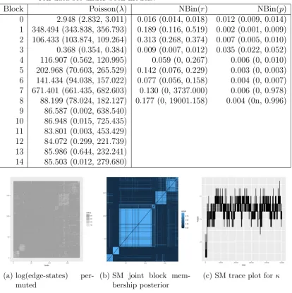
2.2. Simulated data parameter values for each edge-state distribution considered. . . 49

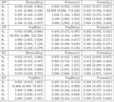
2.3. Mean and 95% credible interval (CI) for parameters of example networks. . . 51

2.4. RubGelman Statistics (and upper bound of 95% confidence in-terval) for each model with 30 independent chains of 5000 iterations for RJMCMC and Dirichlet Process samplers. . . 56

2.5. Parameter estimates and 95% highest posterior density interval for Macaque network. . . 60

2.6. Parameter estimates and 95% highest posterior density interval for Enron data set under both models. . . 62

2.7. Parameter estimates and 95% highest posterior density values for the Stack Overflow network. . . 65

2.8. Model block structure for the Stack Overflow network. . . 65

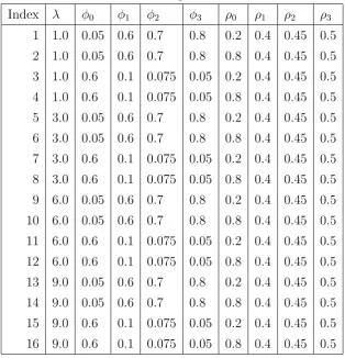
3.1. Parameter settings for simulation study. . . 88

3.2. Number of nodes per community for nc=unequal. . . 88

3.3. Parameter estimates for the mice community data set. . . 94

3.4. Parameter estimates for the mice community data set from the dynSBM (β) and ARSBM (π, ρ). . . 94

4.2. Parameter settings for simulated data sets. . . 117 4.3. Posterior means for SMC and RJMCMC algorithms in simulated

networks. . . 125 4.4. Final time posterior mean and variance for mice network under SMC

and the corresponding estimates for the RJMCMC algorithm. . . . 126

Networks are ubiquitous in modern life: physical networks including roads, rails and pipes carry goods and services. Virtual networks, including telecommunica-tions and the internet, enable sharing of files and messages. Social networks, both online and offline, describe the connections between people and animals. The field of network science is very broad, covering problems such as route-finding on a road network, designing telecommunications networks robust to the failure of connec-tions or finding the most influential member of a social network. The field can be broadly divided based on the characteristics of the network under study. For example, in the network flow problem, the network is considered fixed (the roads are already in place) and an optimal route is sought. In the robust telecommu-nications example, the network is being designed (where should the intersections be placed?). Finally, in social network analysis, often the network structure is un-known and needs to be inferred to answer questions such as influence. This leads to quite different sub-fields of study.

a mechanism under which the network was generated, e.g. small-world networks Watts and Strogatz (1998), whereas statistical models aim to fit a probabilistic model with all the power of assessing fit using statistical inference procedures. The line between mathematical and statistical model is blurred but the literature on both has remained mainly distinct over the past two decades.

Much of the early work on network modelling focused onstatic networks, where information about a network is collected at one point in time, or is summarised to yield a single piece of information between pairs of individuals. A popular and well studied statistical model is the stochastic block model (SBM). This divides the set of nodes into groups, such that nodes in the same group have a similar behaviour in terms of their edge-states. Example application areas for the SBM include determining the friendship groups in social network analysis (Wang and Wong, 1987; Snijders and Nowicki, 1997; Zhao et al., 2011; Newman and Reinert, 2016) and separating the regions of the brain into a number of functional groups (N´egyessy et al., 2006a).

In recent years, models fordynamicnetworks have been developed. These extend static network analysis and models to consider the state of networks through time. An interesting problem is thus to determine if a change in structure has occurred in the network.

This thesis is concerned with changes in the structure of a network. The topic lies at the intersection of network modelling, dynamic network models and changepoint detection. This chapter reviews the fields of network modelling for both static and dynamic networks, and introduces the contributions of each chapter and their position within the statistical literature.

1.1. Modelling networks

is assumed to be generated by some simple probabilistic rule with a small set of parameters. The estimation of such parameters from an observed network can indeed be viewed as a statistical problem, however the term “statistical models” refers to models designed to explain observed data. As such, statistical models allow for standard statistical tools such as goodness of fit tests and the evalua-tion of explanatory power of variables on the formaevalua-tion of edges within a network. This section reviews the literature on both these areas, with a focus on statistical models. Before proceeding with the review, firstly the mathematical concept of a network is defined and notation is introduced.

1.1.1. Notation and definitions

Networks are often conceptualised as mathematical graphs. In such a framework, the interactions of a network are denoted byedges, while the individuals or entities performing the interactions are designated asnodes. A static network N, consist-ing of a set of nodes V and a set of edges E, is written N = (V,E). Statistical analysis of a networkN involves models for the generation of the edges in E. For ease of reference, let ij denote the edge between nodes i and j. Furthermore, denote by Eij the state of edge ij in network N; this is considered random and is the quantity to be modelled. Networks with values for the edges can be viewed as weighted graphs, so in the above notation, the weight of edge ij is the value of

Eij.

be in conversation or not). By allowing every edge to exists, the phrase “the edge between nodes i and j switches state from true to false” is comprehensive.

Some graph-theoretic terms carry over into network modelling: in the case of binary edge-states, the degree of a node is the number of edges in state one for whichiis an end-node. Furthermore, thesize of a binary network is the number of edges in state one. Adegree sequence is the (ordered) list of degrees {di :i∈ V}.

The types of interaction can vary also. In some cases the interaction process may allow for self-interactions. These are calledself-loops. Symmetric interactions, such as “is friends with”, create symmetric networks. In symmetric networks the edge-states have the following relationship: Eij =Eji for all i6=j. If a network is symmetric with no self-loops, then it is modelled as asimple graph. On the other hand, interactions may have a concept of direction, such as “nodei sends node j

an email”; such networks are modelled asdirected graphs.

For a given network N, it is convenient to consider theadjacency matrix. This is the matrix of edge-statesE. If a network contains symmetric edge-states, then Eis a symmetric matrix. Furthermore, if there are no self-loops inN, then Ehas 0 values on the diagonal.

1.1.2. Mathematical models for networks

A mathematical model for a network is mainly concerned with the mechanisms that gave rise to the network via simple rules with few parameters. As such they can be referred to asnetwork growth models. There is an extensive literature on these models, mainly in the domain of statistical physics. Generally, a mathematical model takes some parameters θ which drive some growth mechanism.

Since this thesis is mainly concerned with statistical models, only a few major mechanisms are reviewed here.

The first growth model to appear in the literature is arguably the simple random graph (Gilbert, 1959; Erdos and R´enyi, 1960). In such a model, the set of N

nodes, V, is fixed and binary edge-states are assigned to the edges. In one version of the model, given the nodes, the edge-states are drawn uniformly with some probability p. An alternative version (which is easier to generalise), chooses a network at random from the set of all networks containing a given number of edges. The generalised Erd˝os-R´enyi model chooses a network uniformly at random among among a set of networks with a given set of properties. This generalises the original model since the number of edges is such a property. Another common property is the degree sequence, henceN is chosen from the set of networks with a set degree sequence{d1, d2, . . . , dN}. Interest may lie in some counts of arbitrary sub-graphs called “motifs” for example, the number of connected triples (complete sub-graphs on three nodes).

The following procedure demonstrates the ideas behind the mathematical mod-elling paradigm. To analyse a given networkN, firstly a property or properties P

are chosen and calculated as ˆp = p(N) for each p ∈ P. Secondly, the theoretical properties are calculated for the set of graphs obeying P. Finally, ˆp is compared to its theoretical value. For most properties of interest, the theoretical values are non-analytic, and hence MCMC algorithms to draw from the set of networks obey-ingP have been developed. This is a whole literature in itself, but key algorithms are given in Kolaczyk (2009). For the case of general motifs, first an underlying network generation model must be assumed, then the theoretical distribution for motif counts calculated. This quantity is non-analytic and difficult to approxi-mate, even for the simple Erd˝os-R´enyi model (Picard et al., 2008). Furthermore, without a robust theoretical distribution for motif counts, the use of p-values for model fit is difficult to justify.

networks have the following properties: (i) most nodes have few neighbours, (ii) the neighbourhoods of two neighbours has a large intersection, (iii) the average of the shortest path between any two nodes grows logarithmically in the number of nodes. The work of Watts and Strogatz (1998) classified networks based on the

clustering coefficient and shortest path length. The clustering coefficient measures the tendency for nodes to group together into clusters and attempts to measure (i) and (ii) in the above list. If nodes group together, then the intersection of the neighbourhoods of two nodes in the same group will contain many nodes. The clustering coefficient is defined as the ratio of the number of triplets of nodes with all possible edges to the number of triplets of nodes with two possible edges. This can be seen in a graph as the number of triangles divided by the number of connected triplets.

In an Erd˝os-R´enyi network model, the clustering coefficient is small, together with a short average shortest path length (ASPL). For example, withN nodes and probability of an edge appearingp, such that N p >1, the clustering coefficient is

p and ASPL grows as O(logN) in the limit N → ∞ (Bollob´as, 1998). However, in small-world networks, the clustering coefficient is large with a small ASPL.

The mechanism to generate a small-world network as given by Watts and Stro-gatz (1998) is as shown in Algorithm 1.1. In the first stage a regular lattice network is created. This ensures the network starts with a high clustering coeffi-cient. Secondly, by “rewiring” edges at random (avoiding already existing edges and self loops), the ASPL is greatly reduced. Asβ →1, a Watts-Strogatz network approaches an Erd˝os-R´enyi network. For the case of β = 0, the Watts-Strogatz algorithm yields a lattice: each node has exactly K neighbours and consecutive nodes share K −2 neighbours. In this case, the clustering coefficient is 3(₄₍K_K−₋2)₁₎ which approaches 3

4 for largeK whilst the ASPL is exactly

N

2K. For the case where

β∈(0,1), the ASPL decreases quickly with β, whilst the clustering coefficient re-mains close to the value atβ = 0 and can be shown to be asymptotically equal to

3(K−2)

4(K−1)(1−β)

produces small-world networks.

Algorithm 1.1The generation of a small world network via the Watts-Strogatz algorithm.

Require: Number of nodes N, mean degree K,β ∈[0,1]. Start with node set V ={1, . . . , N} and an empty edge setE. Label N nodes as 1, . . . , N.

for i= 1, , . . . , , N do

For nodes j such that i−j = 1, , . . . , , K mod N, add ij to E.

end for

for i= 1, , . . . , , N do for j =i, , . . . , , N do

With probability β choose a nodek ∈ {j :j 6=i, ij 6∈ E} 6=i. Deleteij from E.

Addik toE.

end for end for

return Network N = (V,E).

Another popular mathematical model for networks is the preferential attachment model. The mechanism generating such networks is often dubbed “the rich get richer”. A well-known algorithm for generating a preferential attachment network is described by Albert and Barab´asi (2002). To generate a network, start with a single edge between two nodes n1 and n2. At each step, a new node ni is added, and an edge betweenni and nj (j < i) is created with probability proportional to the degree ofnj. In such a way, the more edges incident to a node, the more likely it will receive an edge from a new node. This is made concrete in Algorithm 1.2. As such, networks generated from Algorithm 1.2 are likely to contain some nodes with very high degrees, or hubs. Another property of the Albert and Barab´asi (2002) model is the degree distribution: it is scale-free. Specifically P[d(ni) =k] ∝ k−3.

The ASPL can be shown to be asymptotically _{log log}logN_N.

1.1.3. Statistical network models

Algorithm 1.2The generation of a scale-free network via the Barab´asi–Albert algorithm.

Require: Number of nodes N, initial number of connected nodes N0.

Start with node set V ={1, . . . , N0} and empty edge set E =∅.

for i= 2, . . . , N0 do

for j < i do

Addij to E.

end for

Set the degree di =N0 −1.

end for

for i=N0+ 1, . . . , N do

Add node i to V.

for j < i do

Addij to E with probability pij = dj

P

k<idk.

end for

Update the degrees of nodes 1, . . . , i.

end for

return Network N = (V,E) and the degree sequence {di :i∈ V}.

network properties such as average degree, ASPL and clustering coefficient re-ported and discussed.

In this section, some statistical models are reviewed. The change in focus be-tween statistical and mathematical models is on estimation and representation: models must be able to be fit to the data and allow exploration of the effects that explain the data. None of the mathematical models are suited to this.

Three main categories of statistical model have been developed over the last few decades: exponential random graph models (ERGMs), latent space models, and stochastic block models (SBMs). These each mirror classical statistical methods: the ERGM can be viewed as a generalised linear model, latent space models use both observed and latent variables to model the probability of edge-states in the manner of classic latent space models, and SBMs are, at their heart, a mixture model.

mod-els (Wasserman and Pattison, 1996). These are special cases of the more general ERGM which itself is analogous to classical generalised linear models (GLMs).

P[E=e] = 1

Jexp

X

h∈H

θhgh(e)

!

, (1.1)

where gh are functions counting the number of times configuration h appears in e. Equation (1.1) shows the general form of the ERGM, an exponential family

form, for the joint distribution of the adjacency matrix E. The ERGM is based onconfigurations or sub-graphs within the network: for example, the appearance of edges or triangles or k-stars (a set of k edges sharing the same end-node). The hope is that simple structures can explain the observed adjacency matrix e. In Equation (1.1), the configurations of interest are denoted by the set H. For each configuration h, there is an indicator function gh, which counts the number of times configuration h appears in the adjacency matrix e. If θh is non-zero, then theEij are dependent for all i, j in configuration h. This is the main appeal of the ERGM: a certain dependency structure on the appearance of edges in the network can be imposed through a small number of configurations. A further draw of the ERGM framework is the ease with which additional information X on the network can be included, simply specify the conditional distribution of E on X in exponential form with the addition of statistics g depending on e and x. For example, if covariate information on the nodes is available as a vector x with xi the data about node i, then a simple model would be to include additive effects:

g(e,x) =P

ijeij(xi+xj). In this case, the log-odds of the edgeij appearing in the network increases with the covariate values for i and j. Second order terms can be included by comparing the values of xi and xj. In the simplest case, x is discrete and a matching criteria can be used: g(e,x) = P

ijeijI[xi +xj].

The simplest such ERGM assumes that each edge appears independently, with some probability θij for nodes i and j. As such the functions gh for configuration including more than two nodes hasθh = 0 and the model reduces to: P[E=e]∝ expP

ijθijeij

each data point. Setting eachθij =θmakes the further assumption that edges are independent and identically distributed and, in this case, the Erd˝os-R´enyi model is recovered with P[E=e]∝exp(θM(e)).

Although the ERGM has been demonstrated as a very flexible model, being able to incorporate covariate and dependency structures into the model, it does suffer from some problems. The configurations to include must be chosen carefully, since they easily conflict, leading to correlated estimates. For example, the number of triangles will be correlated to the number of edges since the number of edges is at least three times the number of triangles.

The work of Frank and Strauss (1986) posit ERGMs including only terms for the number of triangles and somek-stars (notice this includes the simple model of counts for edges and triangles since an edge is a 1-star). This model is simpler than the full model in Equation (1.1) which should lead to more interpretable results. In practise however, this model yields poor fit to real data due to model degeneracy (Handcock et al., 2003). To overcome such an issue, more terms could be included, but this leads to a large model. Various attempts to rectify this include making a parametric assumption on thek-star terms (Snijders et al., 2006; Robins et al., 2007).

ERGMs. Recent research (Bhamidi et al., 2011; Chatterjee and Diaconis, 2013) provides a framework for the asymptotic analysis of edge-and-triangle ERGMs, and give proofs of model degeneracy. Therefore, despite the potential of such models, ERGMs lack the theoretical underpinnings to be used with confidence.

The latent space models developed by Hoff et al. (2002); Handcock et al. (2007); Hoff (2008a,b); Krivitsky et al. (2009) treat the nodes as exchangeable in the absence of covariate information. This is motivated by the Aldous-Hoover theorem, since if the elementsEij are exchangeable, then they can be expressed in the form:

Eij =h(µ, ui, uj, ξij)

with wherehis a probability,µa constant,ui, uj i.i.d. latent variables (withh sym-metric inui, uj) and ξij i.i.d. pair-specific effects. This still leaves much flexibility via the specification of h. A popular approach is to let ξij be standard Gaussian variates,µto be augmented with covariate information and include latent termsu through some functionα. This leads to a probit-like model in Equation (1.2). The choice of functionα and the latent space U to which ui, uj belong determines the latent effects of the model, analogous to the choice of configurations in the ERGM. Lettingui, uj ∈ {1, , . . . , , κ} together with α(ui, uj) =muiuj for real valued mkl is

similar to the stochastic block model: ifiand j are in groups k and l in the latent space U, then the probit model increases by mkl. An interesting choice for α, U

comes from the social science principle of homophily, where similar individuals are likely to associate with each other. In this case,α is chosen as a distance function on the latent space U, such that nodes close together in latent space are more likely to share an edge.

P[Eij = 1|Xij =xij] = Φ µ+x0ijβ+α(ui, uj)

(1.2)

offer a variety of possible models but it can be difficult to interpret the latent space and the nodes’ positions therein. Those models based solely on a distance-basedα can also suffer in estimation, since the likelihood is invariant to isometric transformations of the latent space coordinates u.

1.1.4. The stochastic block model

Lastly, the stochastic block model (SBM) is reviewed. This is the basis of the research presented in this thesis and, as such, a more rigorous introduction is given for the SBM. The SBM was first posed by Holland et al. (1983); Fienberg et al. (1985); Wasserman and Anderson (1987) as a random graph model. In these, the nodes are split into clusters or blocks, and, given the block memberships, the edge-states are generated from a mixture model. The mixture weights for a given edge-state are determined by the block membership of the end nodes. The main assumption under the SBM is the node-setV can be partitioned intoκblocks such that any node belongs to only one block. Furthermore, edge-states are assumed independent of other edge-states, given the block memberships. Letting E be an adjacency matrix for a network and z denote the block memberships, such that

zik = 1 if node i is assigned to blockk and zik = 0 otherwise, then the SBM may be written in hierarchical form in Equation (2.1).

Z =z|ω∼Multinomial(z|ω) Θkl =θkl∼Beta(θkl|αkl)

Eij =eij|θ,z ∼Bernoulli eij|θzizj

(1.3)

this case, “community” normally refers to a block structure where a node is more likely to share an edge with a node in the same block than one in another block (θkk≥θkl). The most popular fitting procedure in the statistical physics literature is the maximisation ofmodularity. Modularity according to Girvan and Newman (2002) measures the difference between connectivity between blocks and within blocks. Specifically, let Mkl(z,E) = P

ijEijI[zik = 1, zjl= 1] be the counts of edges between block k and l under the block membership vector z. Then the modularity of z is:

Q(z,E) =

κ

X

k=1 Mkk

M −

Pκ

l=1Mkl M

2

.

Maximising modularity with respect tozyields block structures where the density of edges within blocks is higher than between blocks. Notice that modularity maximising methods do not perform inference on the parameters θ, they only recover the block structure z. It has been argued that modularity maximisation is biased compared to maximum likelihood estimation (Bickel and Chen, 2009) although recent work has shown its equivalence to a restricted form of the SBM (Newman, 2016).

A specific form of the SBM, dubbed the affiliation model, has been studied in depth by Snijders and Nowicki (1997); Nowicki and Snijders (2001); Copic et al. (2009). In this case, the parameters θ are reduced to either between-block and within-block parameters as θkk = θw and θkl = θb for k, l ∈ {1, . . . , κ}. The above references discuss technical issues such as fitting the affiliation model and the model degeneracy when all blocks are of the same size.

description lengths (Peixoto, 2013), sequential testing by embedding successive block models with increasing κ (Lei, 2016) and cross validation (Chen and Lei, 2016). These methods all fit an SBM model with a given κ, then do a post-hoc analysis to find an appropriate “final” κ.

An alternative approach is to let κ be random, and infer κ together with the block assignmentsz and parametersθ. Extending the SBM by allowingκto vary leads to the Infinite Relational Model (IRM) (Mørup and Schmidt, 2013). The IRM extends the model hierarchy of the SBM by placing a prior onκ. Specifically in the case of the IRM, a joint prior is placed on κ,z. This takes the form of the Chinese Restaurant Process (CRP) (Gershman and Blei, 2012). On top of this, the parameters θ can be integrated out of the SBM model, leading to efficient collapsed Gibbs sampling algorithms (Mørup et al., 2011; Mørup and Schmidt, 2012, 2013; McDaid et al., 2013)

The IRM extends the SBM by placing a CRP prior on the number of blocks and block memberships. The CRP is a form of Dirichlet process used in clustering (Antoniak, 1974; Anderson, 1991; Escobar and West, 1995; Rasmussen, 2000; Neal, 2000). To cluster a set of points e1, . . . , eN, the CRP assigns each point sequen-tially. Firstly, following the derivation of Gershman and Blei (2012), e1 forms a

cluster labelled 1. After i−1 points are assigned, suppose there are κi clusters. Then,ei is assigned to cluster k proportional to the number of points in cluster k

(fork = 1, . . . , κi) or ei starts a new cluster with probability γ (a model

parame-ter). This process is exchangeable, so the partition defined by the CRP does not depend on the order in which the vertices are assigned to clusters (Gershman and Blei, 2012). The CRP has a similar property to the preferential attachment model in Section 1.1.2: a large cluster is more likely to gain new points. As such, the CRP tends to create partitions where one part is much larger than the others.

and the block memberships are treated as unknown a priori. With this prior, the SBM is extended to the IRM in Equation (1.4)

The IRM can be written as:

κ,z ∼CRP(γ)

θkl ∼Beta(α)

Eij|z ∼Bernoulli θzizj

(1.4)

The posterior distribution of z can be found using a collapsed Gibbs sampler (Mørup and Schmidt, 2013). Note that under such an inference procedure, the θ parameters are treated as nuisance parameters and are integrated out of the model.

So far, only binary edge-states have been considered. This is reflected in the literature, with arbitrary edge-states considered only recently (Jiang et al., 2009; Mariadassou et al., 2010; Ambroise and Matias, 2012). The generalisation to arbitrary edge-states is simple, given the block memberships z, the edge-state E are assumed independent, and the distribution, G, of Eij depends on zi,zj and some parameters θ. These are the core assumptions of the SBM shown in Equation 1.5.

(Eij ⊥⊥Ei0_j0)|z for all i, i0, j, j0 ∈ V

g(Eij|z) =g(Eij|Zi, Zj,θ)

(1.5)

For example, when considering edge-states representing count data, a Poisson distribution may be used forG(Mariadassou et al., 2010) or a Normal distribution for real-valued edge-states (Wyse and Friel, 2012).

1.2. Dynamic stochastic block models

There is a vast literature on dynamic network models, including dynamic exten-sions of the models introduced in Section 1.1.3. Early work in the field started with continuous-time Markov processes with edge-independence (Wasserman, 1980a,b) and stochastic actor oriented models (Snijders and van Duijn, 1997; Snijders et al., 2010). For a full overview see the review paper by Holme (2015). This thesis focuses on dynamic extensions to the stochastic block model, and thus a more comprehensive review of this field is given in this section.

Multiple temporal extensions of the stochastic block model exist. These can be classified in one important way: how the data are collected. In point-process-like models, edge-state data is assumed to be collected with a time-stamp. As such, data sets come in the form of a list of edges with a time point. For example, the list (is, js, ts) for s = 1, . . . , S represents the S observed edges, with the sth observed edge at timets between nodes is and js. Insnapshot models, the edge-state of all edges is collected at predetermined observation times. As such, a series of network “snapshots” are taken at times sayt0, t1, . . . , tS, hence, the data comes in the form of a list of adjacency matrices E0,E1, . . . ,ES.

Point process models for dynamic networks consider data in the form of instan-taneous interactions between the nodes, such as sending an email. The stochastic block model with point process data aims to divide the nodes of the network based on their behaviour over time. Letting Eij(t) be the time-dependent edge-state for the pair of nodes i and j, a point process model, F(λ), is placed on Eij(t) with some parameters λ. The standard form of the stochastic block model can be applied by letting the parameter λ depend on the block membership of nodes i

and j. For example, consider a network of employees at a company and data on when a pair of employees exchange emails. A block structure could form between the departments of the company, such that the rate of email exchange between employees in the same department is higher than across departments.

multivariate hazard model with time-dependent covariates (Butts, 2008; Vu et al., 2011; Perry and Wolfe, 2013). These are Poisson process models with random intensity functions. Another special case of the Poisson process is the Hawkes process. A Hawkes process is a self-exciting point process, whereby the intensity function increases at times close to a point. In this way, the existence of a point makes future points more likely. Specifically, an impulse function is added to the intensity function in a region close to points. In the network case, a multivariate Hawkes process can be used to model the edge-states. Specifically each edgeEij(t) has a rate function λij(t). In the Hawkes process case, an impulse can be added to all intensity functionsλ(t) when a point in a single edge is witnessed. Hawkes process models with the SBM have been developed by multiple authors including Blundell et al. (2012), where there is a Hawkes process per pair of blocks (rather than pair of nodes). In this way an edge-stateEij(t) follows a Hawkes process with parameters determined by the end-nodes. Furthermore, Blundell et al. (2012) use the IRM rather than the SBM, allowing inference to be performed on the number of blocks as well as the underlying processes. Cho et al. (2013) extend the Hawkes process idea further by allowing both a temporal relationship in events (via a Hawkes process) and a spatial component (via a spatial Gaussian mixture model). Linderman and Adams (2014) also propose an SBM with a Hawkes process in non-observed networks, with the view to inferring both the network and its structure through time. The above models all treat the edge-states as point processes, however, research has also been done where the nodes are modelled rather than the edges (Fox et al., 2016).

Point process models are appropriate for instantaneous interactions such as send-ing emails or instant messages, but not so appropriate for interactions with a du-ration such as phone calls or proximity. An alternative dynamic extension of the stochastic block model assumes that data is available in the form of snapshots. These snapshots record the state of all edges in the network at predefined times

such a way that the dynamics of the edges between nodes i and j depends on the block membership of the pair i, j. Models in the literature mainly concern binary edge-states but allow the block membership of nodes to change through time. Therefore, given the block memberships zt at time t, the edge-states are drawn from a Bernoulli SBM. On top of this, the block membership of nodes follows some Markov process. In the works of Fu et al. (2009); Xing et al. (2010); Yang et al. (2011); Xu and Hero (2014), the latent block memberships evolve as a discrete time Markov chain. Specifically, Fu et al. (2009); Xing et al. (2010) propose a mixed-membership SBM where the block memberships are represented as a vectorπit, with πkit denoting the amount to which node ibelongs to block k at time t. The parameter πit is drawn at each time point from a logistic-normal distribution with mean µt and variance Σt. Dynamics are added to the block memberships by assuming that these meansµt evolve through time via an autore-gressive Normal process. On top of this, the parameters governing edge-formation are assumed to follow a similar construction. This choice of a logistic normal dis-tribution makes parameter estimation difficult since no conjugate prior is available and the authors appeal to variational inference. An alternative approach is pre-sented in Yang et al. (2011), where the block memberships are allowed to change over time, but are not mixed-membership. Therefore, a node can belong to only one block per time, but can move between these blocks. In this way, the evolution of block membershipzt is modelled by a discrete time Markov chain with transi-tion matrixA. As such, the probability that a node in block k remains in block k

in consecutive time points isAkk, and the probability of moving from blockk tol

t, the edge-states are drawn from a static SBM with parameterθt, whereθklis the probability of an edge appearing between nodes in block k and l. The inference procedure transforms θt to the real line (via a logit transform) toψt. The ψt are then treated as Gaussian variates with mean Aψt−1 and variance Σt for

parame-ters A and Σ. Given this structure, an extended Kalman filter is applied to get approximate parameter estimates forθt at each time point, then a label switching procedure is used to infer the block memberships zt. There is no explicit model for node transitions.

More recent work by Matias and Miele (2017) extend the SBM by assuming the block memberships evolve as a discrete-time Markov chain. Given the block memberships at time t, the edge-states are drawn from a static stochastic block model. The authors also consider non-binary states; in this case, the edge-state of ij at time t (Eijt) is drawn from a distribution G with a parameter θkl if zit = k and zjt = l. A variational inference procedure is presented to find the maximum likelihood estimates for the parametersθ and block membershipzt through time. Furthermore, the authors discuss model choice to determine the number of blocks and allow for nodes to exit and enter the network during the observation period. The authors discuss the problem of parameter identifiability in this model, where a permutation of the block labels leads to the same inference. As such it can be impossible to follow the path of a node through time, all that can be recovered is the groups at each time point. This problem affects all the models discussed above.

1.3. Contributions

structure in the ARSBM together with inferring the fixed model parameters. This section gives an overview of the contributions made in each of the above chapters. In Chapter 2, two Markov chain Monte Carlo (MCMC) algorithms are presented to draw samples from the posterior distribution of the number of blocks, block memberships and edge-state parameters in a stochastic block model. Historically, research for inference in the stochastic block model has mostly treated the number of blocks as fixed. Of the research where the number of blocks κ is treated as unknown, those which incorporate inference onκ into the main inference (such as the infinite relational model), only conjugate models for the edge-states have been considered. Furthermore, only the Chinese restaurant process prior is used. This is shown to be a rather inflexible choice in Section 2.2.1.

edge-state model, and the negative binomial finds additional structure, since the model is more flexible. Furthermore, a discussion in Section 2.2.1 considers the prior distribution of blocks and block memberships. Traditionally, this is taken as a Chinese Restaurant Process (CRP) which jointly models the number of blocks and block memberships. However, the CRP gives significant weight on block struc-tures dominated by one larger block and multiple small blocks. In Section 2.2.1, it is argued that the Dirichlet Multinomial Allocation (DMA) prior, first used in cluster analysis (Green and Richardson, 2001), is a more flexible model for the number of blocks and block memberships. Specifically, the DMA is a hierarchical model allowing the number of blocks to be specified via an arbitrary distribution with support on a subset of the positive integers. Following this, a prior is placed on the block memberships given the number of blocks. As such, priors can be constructed where the number of blocks can be modelled separately to the block structures. These allow distributions where blocks are expected to be of equal size without influencing the number of blocks; an impossibility under the CRP.

autoregressive edges, a more realistic temporal model is provided, (ii) by setting the model in a continuous time framework dealing with missing data or irregular sampling is simple. The closest available method is the work of Matias and Miele (2017), where dynSBM is proposed. This model sets the block-membership process as a discrete-time Markov chain. Given the block memberships, at each time-point the edge-states are drawn independently from a static SBM model. Compared to Chapter 3, dynSBM cannot handle irregular sampling times without adaptation. Furthermore, no autoregressive behaviour is possible for the edge-states. In the ARSBM, the location of change points is inferred via a reversible jump Markov chain Monte Carlo sampling algorithm. This yields a distribution over change location, providing a quantification in uncertainty of the change points. Current methods, including dynSBM only provide point estimates for block membership and model parameters, or use a variational approximation technique. Such vari-ational techniques are known to be over confident in their maximum likelihood estimates, and thus the uncertainty in parameter estimates provided by current methods is often underestimated (Blei et al., 2017), hence the ARSBM inference is more honest in its parameter uncertainty when compared to currently available methods for dynamic stochastic block models. The ARSBM allows more realistic treatment of dynamic network data by explicitly allowing temporal dependence on previous edge-states. On top of this, the problem of identifying evolutions in block membership is considered; specifically, the problem of detecting if nodes have changed group is tackled. This problem has been considered by other authors both in a Bayesian (Fu et al., 2009; Yang et al., 2011; Xu and Hero, 2014) and a frequentist context (Matias and Miele, 2017), yet these models do not allow for autoregressive terms.

distribution of parameters given the edge-states and block structures to be sepa-rable. This scheme allows for an MCMC within particle filter algorithm (Storvik, 2002; Fearnhead, 2002). Specifically, a Gibbs sampler can be implemented to infer the parameters through time in a rigorous manner within the SMC algorithm. Therefore, the storage requirements of the algorithm are much smaller than the RJMCMC algorithm of Chapter 3. This problem has been attempted (Fu et al., 2009; Xing et al., 2010; Yang et al., 2011; Xu and Hero, 2014), but without the inclusion of autoregressive terms. Hence, as in Chapter 4, applying the ARSBM in a dynamic setting allows more flexible modelling of temporal data by explicitly allowing future edge-states to depend on the past.

2. Arbitrary edge-states and

unknown number of blocks in the

stochastic block model

2.1. Introduction

Statistical analysis of networks has seen much growth in recent years with the in-creasing availability of network data. The term “network” is used in a broad range of research fields. In this paper, a network consists of a set of nodes, which can form pairwise interactions. Each possible interaction is referred to as an edge, with the value of that interaction being denoted as an edge-state. In similar work these are referred to as possible edges and edge-weights. By referring to each possible pair of nodes as an edge, the terminology is more succinct. The aim of statisti-cal network modelling is to describe the edge-states with a probabilistic model, potentially performing inference for model parameters. Such models include the exponential random graph, the class of latent space models and the stochastic block model (SBM). Under the SBM, the set of nodes is partitioned into blocks

such that the edge-state between two nodes depends on their block memberships. For example, an assortative block structure in a network with binary edge-states is formed when nodes in the same block are more likely to have an edge-state of one than between nodes in different blocks.

stochastic block model. The SBM has been studied at least since the 1980s (Hol-land et al., 1983; Frank and Harary, 1982), with attention turning to non-binary edge-states in the 2000s (Jiang et al., 2009; Mariadassou et al., 2010; Ambroise and Matias, 2012). There is a rich literature on the SBM including both Bayesian and Frequentist treatments. Extensions to the SBM include restricting the SBM to only within-block and between-block edge-state distributions in the affiliation network (Snijders and Nowicki, 1997; Nowicki and Snijders, 2001; Copic et al., 2009), multiple-block memberships in the mixed-membership SBM (Airoldi et al., 2008), degree-corrected SBM (Karrer and Newman, 2011), and the infinite rela-tional model (IRM) (Kemp et al., 2006) where the number of blocks is treated as unknown. For a thorough review of the SBM and inference methods see Matias and Robin (2014).

The Bayesian inference procedure we present is applicable to networks with arbitrary edge-states, extending the work of Mørup and Schmidt (2012, 2013) and McDaid et al. (2013). The inference algorithms presented in this paper allow much more flexible modelling than previous work on networks with arbitrary edge-states. Previous authors have only considered conjugate models for edge-states, whereas we allow much more flexibility in the choice of prior by only assuming that (1) samples can be taken and (2) point-wise evaluation is computationally feasible. This greatly broadens the applicability of the stochastic block model to general network data with arbitrary edge-states.

number of blocks (Lei, 2016) and cross validation (Chen and Lei, 2016). These methods all fit multiple SBM models with differing numbers of blocks, then do a post-hoc analysis to choice a final number. Alternatively, treating the number of blocks as a random variable allows inference on the joint distribution of number of blocks, block membership of nodes and model parameters. Extending the SBM by allowing the number of blocks to vary leads to the Infinite Relational Model

(IRM) (Mørup and Schmidt, 2013). The IRM extends the model hierarchy of the SBM by placing a Chinese Restaurant Process (CRP) prior (Gershman and Blei, 2012) on the number of blocks. On top of this, the parametersθ can be integrated out of the SBM model, leading to efficient collapsed Gibbs sampling algorithms (Mørup et al., 2011; Mørup and Schmidt, 2012, 2013; McDaid et al., 2013)

In this paper, the number of blocks is estimated under the later paradigm. Two algorithms are presented to sample from the posterior distribution of the block parameters, block memberships and number of blocks in a stochastic block model. The first algorithm uses the Dirichlet process (DP) sampler (Neal, 2000) to create a Metropolis-within-Gibbs sampler. Given the block memberships, the parameters θ can be updated using a Metropolis algorithm. The block memberships and number of blocks can be updated in turn given the parameter values. This is similar in spirit to the collapsed Gibbs sampler of McDaid et al. (2013) – for a given node i, the posterior probability of belonging to block k is computed with all other parameters fixed. Under the collapsed regime, considering assigningi to a new block k∗ is simple, since the parameters θ have been integrated from the model. In the case of non-conjugate mixture models, this parameter is required to evaluate the likelihood of node i belonging to block k∗. However, notice that in the SBM, if a node is the only member of a block, then such a block contains no edges – any parameter value θk∗ does not affect the likelihood. By drawing

θk∗ from its prior, the proposal and prior densities will cancel, meaningθ_k∗ has no

poor value of θk∗ can decrease the likelihood substantially).

The Gibbs like nature of the DP sampler is not without its pitfalls: the sampler can get “stuck” in local maxima of the posterior. Specifically, in the case of block models, the sampler can be stuck such that two “true” blocks (k, lsay withnkand

nl nodes respectively) are assigned to block m. To reach a better local maxima, the sampler must separate the nodes currently in m to two new blocks matching the true labels k and l. Under the Gibbs sampler, to reach such a state requires moving at least min(nk, nl) nodes. Each of these moves is unlikely, meaning the series of such moves is very unlikely. However, if the sampler proposed allnknodes belonging to the “true” block k to be moved at once, the sampler could “jump” to a place of higher posterior density. Such moves are considered in the second sampler introduced.

The second sampler is inspired by Green and Richardson (2001) – a reversible jump MCMC (Green, 1995) scheme using split and merge proposals to explore the posterior by either combining two blocks, or splitting a block into two. Such split-merge moves avoid the local maxima of the DP sampler, but at the expense of proposing parameter values. Nobile and Fearnside (2007); McDaid et al. (2013) make use of a split-merge proposal, although due to the conjugate models consid-ered, they do not require parameter values θ0. The difficulty in designing a good split-merge algorithm rests on ensuring that parameter values are “matched” when changing dimension.

2.2. Model

The canonical SBM (Holland et al., 1983; Fienberg et al., 1985; Wasserman and Anderson, 1987) considers a network with a fixed number of nodes and blocks denoted asN andκ respectively. The nodes are then partitioned into blocks, with each node belonging to only one block. Let z be the block indicator matrix with

zik = 1 if node i belongs to block k and 0 otherwise. As such zi is a one-of-κ indicator vector. It is assumed that zi is drawn from a Multinomial distribution with parameter ω. The parameter ω governs the block memberships, with ωk being the probability that a node joins block k.

For each pair of blocks, there is an associated parameter ϑkl which governs the probability of an edge-state between nodes in blocks k and l. These parameters can be arranged into a matrix, with diagonal elements ϑkk governing edge-states between nodes both in block k. In the case of undirected edges, the parameter matrix is symmetric with ϑkl = ϑlk. Finally, the edge-states are modelled as independent Bernoulli random variables with probability of success based on the block membership of the nodes. Specifically, the edge-state for edge ij, denoted

Eij, is drawn from a Bernoulli distribution with probabilityϑklwherezik =zjl= 1. Notice this can be written as the quadratic formz_i0ϑzj. This model is summarised in Equation (2.1), first the nodes are assigned to blocks; then given these block memberships, the edge-states are drawn with parameters depending on the block membership of the end-nodes.

z|ω ∼Multinomial(ω, κ)

Eij|ϑ,z ∼Bernoulli(z0iϑzj)

(2.1)

inference must be performed on bothz and ϑ.

The structure of the SBM can be applied to non-binary edge-states, such as count data or a continuous value. In this way, the parameters ϑ apply to some edge-state distribution other than the Bernoulli. As such, a prior distribution other than the Beta is required for the parameters in order to perform inference. A further extension allows ω to be treated as unknown by assigning it a Dirichlet prior. Letting G and G0 be the distribution on the edges-states and parameters

respectively yields the model in Equation (2.2).

ω ∼Dirichlet(γ) z|ω ∼Multinomial(ω, κ)

ϑkl ∼G0(αkl) Eij|ϑ,z ∼G ϑzizj

(2.2)

The IRM treats the number of blocks as unknown. Multiple authors have con-sidered Bayesian inference for the IRM with conjugate models for the edge-states In this case, the parameters governing the edge-states can be integrated out of the likelihood, resulting in a collapsed Gibbs sampler (McDaid et al., 2013). Such an approach is reliant on the conjugate assumptions; hence, only a limited number of edge-state models can be fitted using such algorithms.

In the canonical SBM, there are κ blocks. When considering the block mem-bership of the end-nodes there are κ+1₂

possibilities: the end nodes can be in the same block (κ possibilities) or in different blocks ( κ₂

how many blocks the are. This paper considers a parameterisation between these two extremes: letting θk be the parameters governing edges between nodes in the same block k (of which there are κ), and a global parameter θ0 for edge-states

between nodes in different blocks. In this way the number of parameters is κ+ 1, and grows linearly in the the number of blocks. This model is appropriate for net-works where between block connections are relatively homogeneous; for example in ecological contact networks, where herds of animals remain close together for most of the time, with some between herd interactions. For comparison to the generic SBM from Equation (2.2), let θ be the matrix with parameters with θkl = θ0

and θkk = θk, then the quadratic form zi0θzj picks the parameter governing the edge-state Eij. This may be extended to edge-state distribution G with multiple parameters. Note thatθk is a vector of parameters for the edge-state distribution for edges in blockk (or between blocks ifk = 0). For example, if Grepresents the Gaussian distribution, thenθk = (µk, σk2) represents the mean and variance of the edge-states in block k. In this case, an additional subscript is required onθk such thatθkp is thepth parameter for blockk. In the Gaussian exampleθk1 is the mean

value of edges in block k.

Since the number of blocks κis considered unknown in this paper, a prior must be placed on both the number of blocks and block memberships. Choices for this prior are discussed in Section 2.2.1. Prior parametersα are assigned to the block parametersθ. Meanwhile, letF be a joint distribution for (κ,z) with parameters γ, hence the restricted form of the SBM considered in this paper is shown in

Equation (2.3).

κ,z ∼F(γ, δ) θk ∼G0(α)

Eij|θ,z ∼G(zi0θzj)

2.2.1. Prior for block structure

Under a canonical SBM, the number of blocksκare assumed known. In this case, the standard prior to place on the block allocations z is a Multinomial(ω). In the case where κ is unknown, this can be extended by setting a prior on both

κ and z. A hierarchical prior distribution can be achieved by first setting an arbitrary prior distribution F0 for κ, and then setting a prior for z given κ. One

approach is to let z ∼Multinomial(ω), where ω ∼Dirichlet(γ, κ), the symmetric Dirichlet distribution on theκ−1 simplex. Such a hierarchical prior is referred to as a Dirichlet Multinomial Allocation (DMA) prior (Green and Richardson, 2001). Since a symmetric Dirichlet distribution with parameterγis used, the parameterω can be marginalised out to obtain a prior density for block memberships depending only onκ and γ as shown in Equation (2.4).

f(z|γ, κ) =

Z

ω

f(z|ω)π0(ω|γ)dω

=

Z

ω κ

Y

k=1

N

Y

i=1

ωzik+γ+1

k

Γ(κγ) Γ(γ)κdω = Γ(κγ)

Γ(γ)κ

Qκ

k=1Γ(Nk+γ) Γ(Pκ

k=1Nk+κγ)

(2.4)

whereNk is the number of nodes in block k.

E[κ] =γ(Ψ(γ+N)−Ψ(γ)) (2.5)

However, the marginal distribution on the number of blocks, p(κ), depends on the Stirling numbers of the first kind. The computation of Stirling numbers is non-trivial (Antoniak, 1974). As such, prior specification is more precise under the DMA specification, since it allows a distribution to be placed on the number of blocks independent to the block size distribution.

For use in the following samplers, both the density, and marginal densities for a single node are required. These are available in Equation (2.6) for the DMA and Equation (2.7) for the CRP.

f(zi =l|z¯, η) = η+1

X

κ∗_=η

f(z|κ∗)π0(κ∗|η) π0( ¯z|η) = Γ(γ)

η

Γ(γη)

Γ(γη+M)

Qη

k=1Γ(γ+Mk)

×

Γ(γη) Γ(γ)η

Qη

k=1Γ(γ+Mk+zik)

Γ(γη+M + 1) π0(η|η) + Γ(γη+γ)

Γ(γ)η+1

Qη+1

k=1Γ(γ+Mk+zik)

Γ(γη+γ+M+ 1) π0(η+ 1|η)

# =       

π0(η+ 1|η)B(γ_B+1_(γ,ηγ,M+₎ηγ) if l =η+ 1

π0(η|η) Ml+γ

M+ηγ +π0(η+1|η)

B(γ+1,M+ηγ)

B(γ,ηγ)

1 + Ml

γ

o.w.

(2.6) Where ¯z is the set of nodes without node i, M = N −1 is the number of nodes withouti,η is the number of blocks defined by the set ¯z and Mk is the number of nodes in block k from the set ¯z. As for the CRP:

f(z, κ|γ) = Γ(γ)γ κ

Γ(γ+N) κ

Y

k=1

Γ(Nk)

f(zik = 1|z−i, κ, γ) =

      

N_k0

N−1+γ if k ≤κ, γ

N−1+γ if k a new block.

This section closes with a comparison between the CRP and DMA priors. One downside to using the CRP is that generated blocks structures are skewed towards one large block with multiple smaller blocks. By keeping an explicit DMA prior the possible block structures are more flexible and interpretation of parameters is easier, since they are independent features of the model. Firstly, by choosing a specific prior distribution F0 for κ, much more can be said about the number

of blocks; this allows more informative priors when modelling. Secondly, explicit choices can be made for the distribution of nodes to these blocks viaγ. Therefore, for flexible modelling, the DMA is to be preferred. In this work, the DMA prior is used withF0the distribution obtained by adding one to a Poisson random variable. As a consequence, f0(K =κ) = δ

κ−1_exp(−δ)

(κ−1)! for k = 1,2, . . .. A comparison of block

Block

Node

Block

Node

Block

Node

Node Node Node

IRM

gamma= 1

Block

Node

Block

Node

Block

Node

Node Node Node

IRM

gamma= 5

Block Block

Node

Block

Node

Node Node

DMA

gamma= 1 delta= 5

Block Block

Node

Block

Node

Node Node

DMA

gamma= 5 delta= 5

Figure 2.1.: Comparison of block structures. Top left CRP(1), top right CRP(5). Bottom left: DMA(1,5), bottom right: DMA(5,5).

2.3. Dirichlet process sampler

In this section a Dirichlet process sampler for the restricted SBM is given. This adapts the Dirichlet process sampler for clustering of Neal (2000) for the SBM. Running such a sampler for a large number of steps will draw samples from the posterior distribution of (κ,z,θ). In such a procedure, the block membership of each node is updated in turn. When considering a node i, it is either assigned to one of the current κ blocks, or starts a new block denoted by k∗. For the current blocks, a parameterθk is used from the current state of the sampler when calculating the likelihood. For the new block however, a parameter θk∗ is simply

Neal (2000) introduce a Dirichlet process sampler for clustering with non-conjugate models. When clustering, assigning a data point to a new cluster requires a new parameter θk∗. However, in the case of the SBM, there is a key difference: under

the clustering problem each data point belongs to one component, in the SBM each nodei belongs to one block, which in turn decides the distribution which the

N −1 edges with end-node i follow. This will greatly influence the likelihood of the point being assigned to the new clusterk∗. An interesting property for the re-stricted SBM is that assigning a single node to a new block leaves no within-block edges, hence, any value of θk∗ will not affect the likelihood. This can help the

sampler in exploration, since creating a new block is not down-weighted by poor parameter valuesθk∗, such values may be updated by other moves of the sampler.

The specifics of the algorithm are now discussed.

Firstly, let (κs_,zs_,θs_{) be the state of the sampler after s steps. The process by} which the next states+ 1 is generated is described for each of the componentsκ,z andθ. The update process for parameter valuesθhas been chosen as a Metropolis-Hastings random walk on a transformed scale. In the following this is referred to as “Update”, which takes the current state of the sampler and proposes new values θs+1_{. In the analysis, a Metropolis-Hastings procedure is applied with symmetric}

Gaussian proposals on a transformed scale. That is,θ0_k=m−1_{(m(θk) +σξ) where} ξ is a draw from a standard normal distribution andm is an isomorphism fromΘ

toR.

The difficult part of the Dirichlet process sampler is the update for block mem-berships z and, as a consequence, the number of blocks κ. This makes use of a Metropolis update for each node in turn. Letibe the node whose block member-ship,zi, is to be updated. By choosing the marginal prior as the proposal distribu-tion for the block membership ofi, this will cancel in the acceptance probability. Therefore, the proposed block membership of i is drawn as z_i0 ∼Multinomial(p), where pk = f(zik= 1|z−i). Note that the prior here is marginalised over κ as

Therefore, all analysis with the DP sampler will use a CRP prior in this paper. The marginal density for the CRP is given in Equation (2.7). Next, ifiis proposed to start a new block k0, then a value for θk0 is required for this new block. In this

case, denoteθ0 =θ∪θk0 as the proposed set of parameters. By drawing θ_k0 from

its prior distribution G0, this also cancels in the acceptance probability. On the

other hand, ifzi is currently a member of a singleton blockland zi0 6=l, then block

lis removed from the model. In this caseθ0 =θ\θl. In the case where the number of blocks is unchanged when proposing z_i0, the proposed parameter values θ0 =θ. Finally, θs+1,z_is+1 is set to θ0,z_i0 with probability A in Equation (2.8), and to θs,zs_i otherwise. It remains to compute the acceptance probability. Since updates are proposed from the prior distribution, this cancels in the posterior leaving a likelihood ratio. Recall thatG is the distribution for the edge-states with density functiong, and thus g(E|z,θ) is the likelihood function then:

A(zi →z0i) =

π z_i0|E,zs

−i,θ

0

π zs

i|E,z−si,θs

q(zs i|z

0

i)

q(z0

i|zis) = g E|z

0

i,z−si,θ

0

g E|zs

i,z−si,θs

.

(2.8)

The procedure is summarised in Algorithm 2.3. Note that at a given step a node may start a new block, increasing κ. A node may also be the only node in a block, but then be reassigned to a block containing other nodes, decreasingκ. An important case to consider is when a node i is currently a member of a singleton block, say k: a block with only one node. In such a situation, assigning i to k0 is the same asi starting a new block in terms of the model, since block labels have no impact on the model. A simple remedy is to set the probability of reassigning nodei to block k as zero.

2.4. Split-merge sampler

Algorithm 2.3 Metropolis-within-Gibbs sampler for restricted SBM with un-knownκ: Dirichlet process sampler.

Inputs: Edge-states E, prior parametersα, γ, δ. Draw κ0_,z0 _∼F

0(·|γ, δ).

Draw θ0 ∼G0(·|α).

for s = 1, . . . , S do

Draw θs _{∼Update(·|E, κ}s−1_,zs−1_,θs−1_,α)

Let κs =κs−1

for i= 1, . . . , N do

for k = 1, . . . , κs_{+ 1 do} Let pk =f(zik = 1|z−i)

end for

if i currently belongs to a singleton block k then

Let pk = 0

end if

Draw z_i0 ∼Multinomial(p)

if z_i0 =κs+ 1 then

Draw θκs₊₁ ∼G₀(α)

end if

Calculate A from Equation (2.8) Draw Y ∼Bernoulli(A)

if Y = 1 then

Let zs_i =z0_i

else

Let zs i =z

s−1

i

end if

Letκs ₌P∞

k=1I

h PN

i=1z

s ik >0

i

end for

Store sample (zs_,θs_).

introduced in Section 2.3. Both methods draw samples from the posterior distri-bution of (κ,z,θ). However, the split-merge sampler can perform more drastic changes to the state space compared to the Dirichlet process sampler. This can have major benefits when exploring the posterior distribution. For example, the block membership of each node is updated in turn under the Dirichlet process sampler; this can lead to cases where it is difficult to separate nodes which should belong to different blocks. Consider two “true” blockskand l withnk ≥nl nodes. Furthermore, consider a states of the DPS where all nodes in blocks k and l are assigned to one blockks (which contains only these nodes). To separate the nodes withinks to the true blocks k and l requires at least nl steps, each of which takes the nodes assigned to ks _{and assigns them to a new block l}s_{. However, each of} these moves is quite unlikely: especially if the parametersθk,θl are close toθ0. On