Problem-driven Scenario
Generation for Stochastic
Programs
Submitted for the degree of Doctor of Philosophy
at Lancaster University
Jamie Fairbrother, MMath, MRes
Abstract
Stochastic programming concerns mathematical programming in the
pres-ence of uncertainty. In a stochastic program uncertain parameters are
mod-eled as random vectors and one aims to minimize the expectation, or some
risk measure, of a loss function. However, stochastic programs are
computa-tionally intractable when the underlying uncertain parameters are modeled
by continuous random vectors.
Scenario generation is the construction of a finitediscreterandom vector to use within a stochastic program. Scenario generation can consist of the
discretization of a parametric probabilistic model, or the direct construction
of a discrete distribution. There is typically a trade-off here in the number
of scenarios that are used: one must use enough to represent the uncertainty
faithfully but not so many that the resultant problem is computationally
in-tractable. Standard scenario generation methods aredistribution-based, that is they do not take into account the underlying problem when constructing the
discrete distribution.
In this thesis we promote the idea of problem-basedscenario generation. By taking into account the structure of the underlying problem one may be
able to represent uncertainty in a more parsimonious way. The first two
papers of this thesis focus on scenario generation for problems which use a
tail-risk measure, such as the conditional value-at-risk, focusing in particular
driven approach to scenario generation for simple recourse problems, a class
of stochastic programs for minimizing the expected shortfall and surplus of
Contents
Abstract iii
Declaration ix
Preface xi
I
Introduction
1
Background 3
1 Introduction . . . 3
2 Stochastic Programming . . . 3
2.1 General Stochastic Programs . . . 3
2.2 Two-stage stochastic linear programs . . . 6
3 The Basic Newsvendor Problem . . . 9
4 Risk Measures and Conditional Value-at-Risk . . . 12
4.1 General Risk Measures . . . 12
4.2 Conditional Value-at-Risk . . . 14
5 Scenario Generation . . . 20
5.1 Introduction . . . 20
5.2 Sampling Approaches . . . 21
5.3 Optimal Discretization . . . 30
5.5 Problem-Driven Scenario Generation . . . 41
Thesis Summary 47 References . . . 50
II
Papers
55
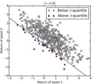
A Scenario Generation for Stochastic Programs with Tail Risk Mea-sures 57 1 Introduction . . . 592 Tail risk measures and risk regions . . . 63
2.1 Tail risk of random variables . . . 63
2.2 Risk regions . . . 66
3 Scenario generation . . . 73
3.1 Aggregation sampling and reduction . . . 74
3.2 Alternative approaches . . . 76
4 Consistency of aggregation sampling . . . 78
4.1 Uniform convergence of empiricalβ-quantiles . . . 78
4.2 Equivalence of aggregation sampling with sampling from aggregated random vector . . . 81
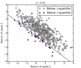
5 Risk regions for the portfolio selection problem . . . 86
5.1 Problem statement and brute force aggregation . . . 86
5.2 Non-risk region for elliptically distributed returns . . . 90
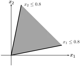
5.3 Non-risk region with convex constraints . . . 93
6 Numerical tests . . . 94
6.1 Experimental Set-up . . . 95
6.2 Results . . . 96
7 Conclusions . . . 96
A Continuity of Distribution and Quantile Functions . . . 99
B Convex cone results. . . 103
1 Introduction . . . 115
2 Portfolio selection and risk regions . . . 119
2.1 Tail risk measures and risk regions . . . 119
2.2 Risk regions for elliptical distributions . . . 124
3 Projections and the conic hull . . . 126
3.1 Conic hull of feasible region . . . 126
3.2 Projection onto a finitely generated cone . . . 129
4 Scenario generation . . . 130
4.1 Aggregation sampling and reduction . . . 130
4.2 Approximation of risk regions . . . 133
4.3 Ghost constraints . . . 135
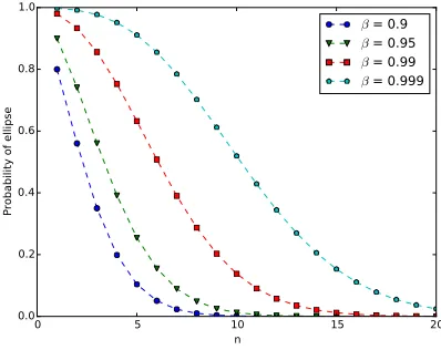
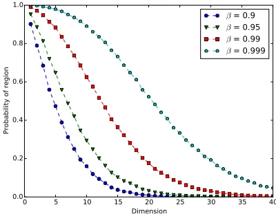
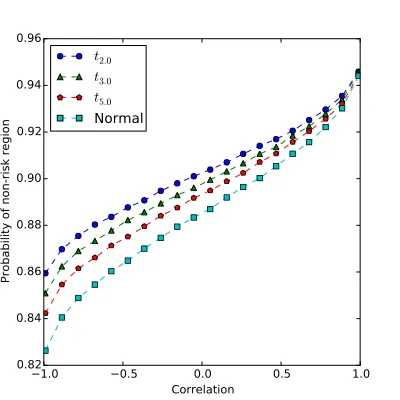
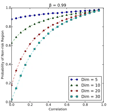
5 Probability of the non-risk region. . . 136
6 Numerical tests . . . 138
6.1 Experimental set-up . . . 139
6.2 Probability of non-risk region with quota constraints . . 141
6.3 Aggregation sampling . . . 142
6.4 Aggregation reduction . . . 145
7 Case study . . . 146
8 Conclusions . . . 152
A Reduction proportion tables . . . 154
B Aggregation sampling tables . . . 157
C Reduction error tables . . . 162
References . . . 165
C Scenario Generation for Newsvendor Problems 169 1 Introduction . . . 171
2 Preliminaries. . . 173
2.1 Wasserstein distance . . . 174
3 The univariate newsvendor problem . . . 177
4 General case . . . 179
4.1 Inactive Components. . . 180
4.2 Scenario generation . . . 182
5 Simple recourse problems . . . 185
6 Numerical Test . . . 188
7 Discussion and Future Work . . . 190
A Numerical Test Problem Data . . . 191
References . . . 192
Declaration
I declare that the work in this thesis has been done by myself and has not
been submitted elsewhere for the award of any other degree.
Preface
Uncertainty is a key feature of many real-world decision making problems.
In portfolio selection problems one has to choose how to invest capital in
fi-nancial instruments with uncertain returns; in inventory problems one must
choose quantities of stock without knowing the future demand. Scenario
generation is concerned with the representation of uncertainty in a form
ap-propriate for mathematical optimization. In particular, uncertain quantities
must be represented by a finite number of possible future realizations, or
scenarios, and one must specify a probability for each of these.
Typically the greater the number of scenarios one uses, the more reliable
the solution that the optimization problem yields, but the more difficult the
problem is to solve. It is therefore desirable to represent the uncertainty as
concisely as possible. Standard scenario generation methods are distribution-based. That is, they construct scenario sets which faithfully reflect the set of future possibilities. The aim of this thesis is the design of problem-based sce-nario generation methods. These are methods which take advantage of the
underlying structure of an optimization problem to provide a more
parsi-monious description of uncertainty. This may mean generating scenario sets
which, in a probabilistic sense, do not accurately represent the distribution of
future possibilities, but which yield near-optimal decisions to our problem.
The motivation for this thesis came from my supervisor Stein Wallace and
Preface
property-matching scenario generation. These methods consist of
construct-ing scenario sets which have prescribed statistical properties. Crucially, these
methods work on the premise that a given decision-problem will only
re-act to certain statistical properties, and in this sense, can be considered to
be problem-based. However, with these methods it is not usually clear a priori which properties are important to a particular decision problem and one has to resort to an empirical investigation to determine this. The aim of
this project was therefore to develop methods which could be proven
math-ematically to be adapted to a particular problem. For this purpose my other
supervisor, Amanda Turner, was enlisted to the project for her expertise in
probability theory.
The first two papers of this thesis concern decision problems which
in-volve tail risk measures. These are problems in which one attempts to
miti-gate or reduce the chance of extreme losses. The first paper is more general
and theoretical in content, and was primarily written in collaboration with
Amanda. The second paper, written primarily with Stein, is focused on
port-folio selection, and how the methodology proposed in the first paper could be
applied to realistic problems. The third and final paper of this thesis relates
to a class of inventory problems, and although it was more of an
indepen-dent piece of work, has benefited much from discussions with both of my
supervisors.
And so a big thank to both of my supervisors. Stein, for his enthusiasm
and insight, and whose flair for analogies would often be employed to make
me see the bigger picture. Amanda, for her optimism and mathematical
expertise, whose keen eye would often catch the flaws, subtle and unsubtle,
in my own mathematical logic.
It has been a privilege to have undertaken this research at the STOR-i
centre for doctoral training at Lancaster University. STOR-i has an engaged
and collegial community of students who have enthusiastically developed
regular forums, training events, and masterclasses organized by them and
staff have broadened my knowledge and skills well beyond the contents of
this thesis. There are too many people to thank here individually for their
work, collaboration and companionship, but I would like to mention my
colleagues Chris Nemeth, Tim Park and Shreena Patel, with whom I joined
STOR-i, for their friendship over these short few years.
Jamie Fairbrother
Part I
Background
1
Introduction
In this chapter we cover the preliminary material required for the reading of
this thesis. This introduction is by no means exhaustive; its aim is to simply
describe the general context of the research and provide some details on the
results we will implictly rely upon. In Section2we give a brief overview of stochastic programming, in Sections3and4we present specific problems in stochastic programming: the newsvendor problem and conditional
value-at-risk, two problems which feature prominently in our research papers. Finally,
we end this chapter with a broad review of scenario generation methods in
Section5.
2
Stochastic Programming
2.1
General Stochastic Programs
Stochastic programming concerns optimization in the presence of uncertainty.
In the most general form a stochastic program consists of a real-valued
ran-dom vector ˜ξ(ω)∈Ξ⊂Rddefined on a probability space(Ω,A,P), a
deter-ministic set of feasible decisionsX ⊂Rk, and alossfunction f
0:Rk×Rd→R∪ {+∞}
pro-gram is to minimize the expectation of the loss function subject to
determin-istic constraints and constraints in expectation:
minimize
x EP
f0 x, ˜ξ(ω) (1)
subject toEPfi x, ˜ξ(ω)≤0, i=1, . . . ,m
x∈ X. (2)
Through the use of indicator functions, the constraints in expectation become
probability constraints. These are useful in mitigating against extreme events
which cannot reasonably be completely precluded (see [1] for instance). This relatively simple form belies the modeling flexibility of stochastic
programs and the difficulty of their solution. For instance, the two-stage
stochastic linear program (SLP) has the following form:
minimize
x c
Tx+E
PQ(x, ˜ξ(ω)) (3)
subject toAx≤b x≥0 where
Q(x,ξ) =min{qTy : Wy=h−Tx, y≥0}, (4)
andy,q∈Rt, h∈Rs, W∈Rs×t,T∈Rs×kand finally
ξ= (q,W,h,T).
This type of problem models the situation where one has to make a
strate-gic decision in the presence of uncertainty, followed by a corrective orrecourse
action once the values of uncertain parameters are fixed, and which incurs
its own costs. The minimization in (4) is referred to as the recourse problem. The interpretation of the elements of the recourse problem is difficult as these
themselves are constructed from underlying blocks of variables or
parame-ters within the recourse problem. In addition, some of the components of the
random vector ˜ξ(ω) = (q(ω),W(ω),h(ω),T(ω))may be fixed.
For clarification we present a concrete example of a simple two-stage
which must produce and delivery some commodity to a group of customers
J. The aim of this problem is to decide on commodity capacities for each facility in such a way which minimizes the combined costs setting up the
facilities, and the future costs of transporting the commodity and of rejected
demand. The mathematical formulation follows:
Parameters:
ci=unit cost of capacity for facilityi
fij=unit cost of transporting commodity from facilityito customerj
rj=unit rejection penalty for unsatisfied demand for customerj
dj(ω) =stochastic demand of customerj
Decisions:
xi =capacity of facilityi
yij(ω) =amount of commodity to transport from facilityito customerj
zj(ω) =rejected demand of customerj
minimize
x≥0
∑
i∈Icixi+EP[Q(x,d(ω))]whereQ(x,d)is the optimal value to the following linear program: minimize
y,z≥0 i∈I
∑
,j∈Jfijyij+∑
j∈Jrjzjsubject to
∑
i∈Iyij+rj=djfor allj∈ J, (demand satisfied)
∑
j∈J
yij ≤xi for alli∈I. (capacity not exceeded)
The recourse problem of this stochastic program is the problem of
minimiz-ing the flow of the commodity from the facilities to the customers.
Compar-ing this formulation to the general one in (4), we note that the only stochastic element of ˜ξin this case ish.
For completeness, we mention also that the problem (1) also encompasses
stochastic process(ξ˜1(ω), . . . , ˜ξT(ω)), and one must make recourse decisions
as each set of values ˜ξt(ω) in the process is revealed. An example of this
problem type is the multistage stochastic unit commitment problem [2]. The most general form of multistage stochastic program is the following:
minimize
x1∈X1 f10(x1) +E
φ1(x1, ˜ξ1)
where for t = 2, . . . ,T the function φt−1 x1, . . . ,xt−1, ˜ξ1, . . . , ˜ξt is defined implicitly as the optimal value to the following stochastic program:
minimize xt ft0
(xt) +Eξt˜|ξ˜t−1φt x1, . . . ,xt, ˜ξ1, . . . , ˜ξt
subject to fti x1, . . . ,xt−1, ˜ξ1, . . . , ˜ξt−1≤0, i=1, . . . ,mt
xt∈ Xt.
where ˜ξ = (ξ˜1, . . . , ˜ξt−1)andXtare deterministic sets of feasible decisions.
2.2
Two-stage stochastic linear programs
The research in this thesis mostly relates to two-stage SLPs. Here we present
some terminology related to and properties of this type of problem. For a
detailed overview of this type of problem see [3, Chapter 3].
The functionQ(x,ξ)as defined in (4) is referred to as therecourse function,
whileQ(x) :=E[Q(x,ξ)]is the expected recourse function. By convention,
when the mathematical program which defines the recourse function in (4) is infeasible, we set its value to+∞. We denote the set of solutionsxfor which the Q(x,ξ) is feasible for allξ ∈ Ξ by K, that is K = {x ∈ Rk : Q(x,ξ) <
+∞for allξ∈Ξ}.
Similarly, if problem (4) is unbounded below then we set the value to be −∞. Note that ifQ(x0,ξ) =−∞for some x0 ∈RkthenQ(x,ξ) =−∞for all
follows:
maximize π∈Rs
(h−Tx)Tπ
subject toWTπ≥q.
If we haveQ(x0,ξ) = −∞for somex0 ∈Rk then this dual program is
infea-sible for x0, but given that the constraints of this problem do not involve x, it must then be infeasible for all x ∈Rk, in which caseQ(x,ξ) =−∞for all
x∈Rk.
A decisionxis considered to be feasible for the problem (3) ifQ(x, ˜ξ)<+∞
with probability 1, or equivalently, ifQ(x)<+∞. Note that this condition is slightly weaker than the constraintx∈K.
The following result concerns the convexity of the recourse function:
Theorem 2.1. Assuming the recourse function Q(x,ξ)defined in(4)is not
identi-cally−∞, it is:
1. a piecewise linear convex function in(h,T); 2. a piecewise linear concave function in q;
3. a piecewise linear convex function in x for all x∈K.
Proof. We just prove that Qis convex in x. The proofs that Qis convex in (h,T) and concave in q are similar. For the proofs of piecewise linearity, see [3].
Fixξ∈Ξ. IfQ(x,ξ) =−∞for somexthen the result is immediate as the
function is identically −∞, so we assume that this is not the case. Now, let
x1,x2 ∈Kand y1,y2be corresponding solutions to the problem (4). We first
show that the problem (4) is feasible forx=λx1+ (1−λ)x2:
W(λy1+ (1−λ)y2) =λWy1+ (1−λ)Wy2
=λ(h−Tx1) + (1−λ)(h−Tx2)
Finally,
Q(λx1+ (1−λ)x2,ξ)≤qT(λy1+ (1−λ)y2)
=λqTy1+ (1−λ)qTy2
=λQ(x1,ξ) + (1−λ)Q(x2,ξ),
where the first inequality follows from the fact thatλy1+ (1−λ)y2is a
fea-sible solution to the recourse problem.
The recourse function is not convex or concave as a function of the matrix
W. Thus, if the matrixW is non-stochastic, that isW(ω) ≡W, the
stochas-tic program is more tractable. The problem in this case is said to have fixed
recourse. In particular, if a problem has fixed recourse, it follows from
Theo-rem2.1, that the expected recourse function is convex.
The evaluation of the expected recourse function, and thus solving the
problem (3), is typically analytically and numerically intractable when the random vector ˜ξ has a continuous distribution. However, when the
distri-bution is discrete with mass points ξs = (qs,hs,Ts) for s = 1, . . . ,n and corresponding probabilities(ps)ns=1, this evaluation reduces to a summation, and the optimization problem to a linear program:
minimize
x c
Tx+
∑
n i=1psqTsys subject toAx≤b
Wys =hs−Ts fors=1, . . . ,n
x,y≥0
Although this can be solved using standard linear programming, specialized
algorithms exist which exploit the structure of this program, for example the
L-shaped decomposition [4].
In paper C of this thesis we study a particular type of fixed recourse called
simple recourse, which has the following form:
This function can be trivially rewritten as follows:
Q(x,ξ) =qT+(Tx−ξ)++qT−(ξ−Tx)+
where x+ = max(x, 0) and the operator is applied element-wise. A sim-ple recourse problem can thus be interpreted as follows: the vector Tx can be thought of as the availability of a set of resources, ξ the corresponding
random demands for those resources, andy+,y− the surplus and shortfalls, respectively of the resources with respect to this demand. The vectorsq+and q− are then considered to be unit holding costs, and rejection costs, respec-tively.
An important property of simple recourse is theirseparability. That is, the recourse function can be decomposed as follows:
Q(x,ξ) =
d
∑
i=1
Qi(x,ξ)
where
Qi(x,ξ) =q+i(Tix−ξi)++q−i(ξi−Tix)+,
andTi denotes thei-th row of the matrixT. This feature is exploited in more specialized solution algorithms, see [5] for instance. We also make use of this property in Paper C.
3
The Basic Newsvendor Problem
The newsvendor problem is a univariate decision problem which concerns
the inventory level of some product subject to an uncertain demand. The
name newsvendor problem has been given to this as it aptly models the
sit-uation of a newsvendor who must decide upon a stock of newspapers to
order to satisfy a daily uncertain demand. This problem is an example of
a two-stage stochastic linear program with simple recourse, and it is used
However, as will be seen in Section 4 the newsvendor problem is also in-timately related to conditional-value-at-risk. In this section we define this
problem, state its optimal solution, and give a detailed proof of this. A more
in-depth study of this model, including its applications and extensions can
be found in the classic textbook [6].
In the newsvendor problem, shortfall of stock relative to the demand
in-curs a unit rejection cost of R > 0. Similarly, a surplus of stock incurs a holding cost h > 0. The aim of the problem is to choose an inventory level which will minimize the total expected cost. If ˜ξ is a random variable
repre-senting demand, andx∈Ris the inventory of the product, then this problem can be written as follows1:
minimize x∈R E
Q(x, ˜ξ)
whereQ(x, ˜ξ) =min{hz++Rz−: x−ξ˜=z+−z−, z+,z− ≥0}. For convenience, we rewrite the recourse functionQ(x, ˜ξ)in the following
form:
minimize x∈R hE
h
x−ξ˜+
i
+REh ξ˜−x+
i
(5)
Note that the objective function E
Q(x, ˜ξ) is convex by the results in
Section 2.2. The set of minimizers of E
Q(x, ˜ξ) can be written in terms
lower and upper quantiles of the random variable ˜ξ. The lower quantile, or
simply the quantile2of a random variable ˜ξfor 0<β<1 is defined to be:
ξβ=inf{x ∈R:P ξ˜≤x≥β},
similarly upper quantile is defined as follows:
¯
ξβ=inf{x ∈R:P ξ˜≤x>β}.
1The above interpretation of this problem requires that the solution satisfiesx≥0. However,
as will be seen, if the random variable ˜ξ is almost surely non-negative then the solution is
guaranteed to be non-negative so we do not need to explicitly enforce this constraint.
2The lower quantile of a random variable when considered as a function ofβis also referred
Proposition 3.1. The set of minimizers of E
Q(x, ˜ξ) is the following compact
interval:
I= [ξ R
R+h, ¯ξRR+h].
Proof. Note first that forx0 <x we have
Eh x−ξ˜+i =
Z
(−∞,x]
(x−ξ)P(dξ) =
Z
(−∞,x]
(x−x0)−(ξ−x0)P(dξ)
= (x−x0)P ξ˜≤x+
Z
(−∞,x0](x
0−
ξ)P(dξ)−
Z
(x0,x](ξ−x
0
)P(dξ)
= (x−x0)P ξ˜≤x+E
h
x0−ξ˜+i
−
Z
(x0,x](ξ−x
0)P(d
ξ).
Similarly,
Eh ξ˜−x+i =
Z
(x,+∞)(ξ−x)P(dξ) =
Z
(x,+∞) (ξ−x
0)−(x−x0) P(dξ)
=
Z
(x0,+∞) ξ−x
0 P (dξ)−
Z
(x0,x](ξ−x
0
)P(dξ)−(x−x0)P ξ˜>x
=E
(ξ˜−x0)+−
Z
(x0,x]
(ξ−x0)P(dξ)−(x−x0)P ξ˜>x.
Now,
E
Q(x, ˜ξ)=EQ(x0, ˜ξ)+ (x−x0) hP ξ˜≤x−RP ξ˜>x
−(h+R)
Z
(x0,x](ξ−x
0)P (dξ)
=E
Q(x0, ˜ξ)+ (h+R)(x−x0)
P ξ˜≤x
− R
h+R
−(h+R)
Z
(x0,x](ξ−x
0)P(d
ξ). (6)
To show that the values in the above interval minimizeE
Q(x, ˜ξ)we
com-pare the value of this function for different values ofxandx0using (6). First, let x0∈ Iand x>ξ¯ R
R+h. By the definition of the upper quantile function, the second term in (6) is strictly positive, also
Z
(x0,x](y−x
0)P(dy)<(x−x0)P x0< ˜
ξ≤x
= (x−x0)
P ξ˜≤x
− R
R+h
hence E
Q(x0, ˜ξ) < EQ(x, ˜ξ). Similarly, if x0 < ξ R
R+h and x ∈ I, it can be shown thatE
Q(x, ˜ξ)≤EQ(x0, ˜ξ). SinceEQ(x, ˜ξ)is convex, it just
remains to be shown that it is constant onI. Suppose Iis not a single point, thatx0 =ξ R
R+h andx∈ Iwithx >x
0. Note that ifIis not a single point then we must havePξ˜≤ξ R
R+h
= RR+h. Ifx<ξ¯ R
R+h thenP x
0< ˜
ξ≤x=0 and
by (6) we see that we must haveEQ(x, ˜ξ)=EQ(x0, ˜ξ). Ifx=ξ R R+h, then R
(x0,x](ξ−x0)P(dξ) = (x−x0)
P ξ˜≤x
−RR+h and again using (6) we have thatE
Q(x, ˜ξ)=EQ(x0, ˜ξ)as required.
4
Risk Measures and Conditional Value-at-Risk
4.1
General Risk Measures
Throughout this section will denote by Z a random variable in R which represents some loss. For our purposes, a risk measure is simply a functional
on a space of random variables.
Definition 4.1 (Risk Measure). Let(Ω,F,P)be a probability space, and V be a non-empty set ofF-measurable real-valued random variables. Then, a risk measure is some functionρ:V→R∪ {∞}.
However, for a risk measure to be useful it should in some way quantify
the danger of large losses3. The quintessential example of a risk measure
is the variance of a random variable and was first used in [8] for portfolio selection problems. A small variance implies a small probability of extreme
losses by Chebyshev’s inequality:
P(|Z−E|Z|| ≥α)≤ Var(Z) α2 .
3The recent paper [7] which proposes a more general framework for measures of risk and
deviation, gives the following more specific characterization: a risk measureρshould “model
Xis “adequately”≤Cby the inequalityρ(Z)≤C”, where C is some loss one wishes not to
The use of variance as a measure of risk is problematic for a few reasons. The
foremost of these is perhaps that variance penalizes large profits as well as
large losses. As a consequence, in the case where the returns of financial
as-sets are not symmetrically distributed, using the variance can lead to patently
bad decisions; for instance, a portfolio can be chosen in favor of one which
al-ways has higher returns (see [9] for an example of this). This particular issue can be overcome by using a “downside” risk measure, that is one which only
depends on losses greater than the mean, or some other specified threshold.
For example the semi-variance [10, Chapter 9], or mean regret [11]:
SemiVar(Z) =Eh|Z−E[Z]|2+i MeanRegretτ(Z) =E[|Z−τ|+]
The semi-variance measures the deviation of losses greater than the mean,
whereas the mean-regret calculates the average loss exceeding some levelτ.
The paper [12] introduced the idea of acoherentrisk measure which is a risk measure which satisfies the following properties:
• (Positive homogeneity)ρ(λZ) =λρ(Z)forλ≥0
• (Translation invariant)ρ(Z+a) =ρ(Z) +afor anya∈R
• (Subadditivity)ρ(Z1+Z2)≤ρ(Z1) +ρ(Z2)
• (Monotonicity) IfZ≥0 thenρ(Z)≥04
Each of these has interpretations in finance, for instance ifZ represents the loss associated with the return of a portfolio, the subadditivity property
ensures that a risk measure favors diversification of portfolios. See [12] for more details. These properties also ensure that a risk measure has desirable
mathematical properties. In particular subadditivity and positive
homogene-ity directly imply that a risk measure is convex.
4This differs from the corresponding axiom in [12] whereZis interpreted as utility rather
4.2
Conditional Value-at-Risk
We now concentrate on a risk measure known as theconditional value-at-risk, as this is the risk measure we use for our numerical experiments.
Denote by 0 < β < 1 a risk level. By GZ we denote the distribution function ofZ, that is
GZ(z) =P(Z≤z).
ByGZ−1we denote thegeneralized inverse distribution function, orquantile func-tion, ofZ, that is
GZ−1(β) =inf{z∈R:GZ(z)≤β}.
We will assume that the random variableZhas finite mean.
The β Value-at-Risk , or β-VaR, is a risk measure simply defined to be
theβ-quantile of a random variable, that isβ-VaR(Z) =GZ−1(β). Theβ-VaR
has been widely used in finance [13], and it has the convenient interpretation of representing the amount of capital required to cover up to β×100% of
potential losses. However, the β-VaR has some undesirable properties: it is
not coherent and is generally intractable in an optimization context.
The β Conditional Value-at-Risk, or β-CVaR, is a risk measure which
dominates theβ-VaR and overcomes its major deficiencies. It can be thought
of as the conditional expectation of a random variable above the β-VaR,
which is indeed the case for continuous random variables, but the general
definition is more technical. The β-VaR and β-CVaR for a continuous
ran-dom variable are illustrated in Figure1.
The β-CVaR was first proposed in [14], and can be defined in several
ways. We use the following definition which is the most relevant in the
context of optimization.
Definition 4.2(β-CVaR).
β-CVaR(Z) =min
α∈R
{α+ 1
1−βE
h
(Z−α)+
i
Density
Loss
Fig. 1:Theβ-VaR andβ-CVaR of a continuous random variable
The definition ofβ-CVaR given in (7) is intimately related to the
newsven-dor problem presented in Section3. Settingh= (1−β)andR=βin (5) and
usingαin place of x, the objective function of the newsboy problem can be
rewritten as follows:
(1−β)E
h
(α−Z)+
i
+βE
h
(Z−α)+
i
= (1−β)E(Z−α)+−(Z−α)+βE
h
(Z−α)+
i
= −(1−β)E[Z] + (1−β)α+E(Z−α)+
= −(1−β)E[Z] + (1−β)
α+ 1
1−β E
h
(Z−α)+
i
.
Thus, calculating theβ-CVaR is equivalent to solving a newsvendor problem.
Sometimes the conditional value-at-risk is referred to as theexpected short-fall. As the name suggests, this quantity is usually defined with respect to lower tail of a random variable representing profit, rather than the upper tail
of a random variable representing loss as we have done. The following
alter-native characterizations ofβ-CVaR were originally given in [15] in relatation
to the expected shortfall. We restate and prove these results with respect to
the upper tail of the distributions rather than lower tails.
i 1−1βEhZ1{Z≥G−1 Z (β)}
i
−G−Z1(β)
β−P
Z<G−Z1(β)
ii 1−1βRβ1GZ−1(u)du
From the first of these characterizations it is clear that whenZ is contin-uous, we have β-CVaR(Z) = E[Z|Z≥β-VaR(Z)]. The second
characteri-zation is written purely in terms of the quantile function of the distribution
and allows us to easily placeβ-CVaR in a wider collection of risk measures
we callβ-tail risk measures as will be seen in Paper A of this thesis.
Proof. We first show that the first characterization is equivalent to (7). Noting the equivalence of calculating the β-CVaR with the newsvendor problem,
and using Proposition3.1, we see that the minimization in (7) is achieved for
α=G−Z1(β). Hence, β-CVaR=G−Z1(β) + 1
1−βE
Z−GZ−1(β)
+
=G−Z1(β) + 1
1−β
Z
[GZ−1(β),+∞)
z−G−Z1(β)
P(dz)
=G−Z1(β) + 1
1−β
EhZ1{Z≥G−1 Z (β)}
i
−G−Z1(β)P
Z≥GZ−1(β)
= 1
1−β
EhZ1{Z≥G−1 Z (β)}
i
+G−Z1(β)
1−β−P
Z≥G−Z1(β)
= 1
1−β
EhZ1{Z≥G−1 Z (β)}
i
−G−Z1(β)
β−P
Z<G−Z1(β)
.
Thus, the first alternative characterization is proved.
To verify the second alternative formulation, we show that it is equivalent
to the first. LetU∼Uniform(0, 1)and defineZ0 =G−Z1(U)∼Z. Note that, {U≥β}={Z0≥G−Z1(β)} \
{U<β} ∩ {Z0 =GZ−1(β)}
(8)
and so
1{U≥β}=1{Z0≥G−1
Now,
Z 1
β
G−Z1(u)du=EhZ01{U≥β}
i
=EhZ01{Z0≥G−1 Z (β)}
i
−EhZ01{Z0=G−1
Z (β)}∩{U<β}
i
=EhZ01{Z0≥G−1 Z (β)}
i
−G−Z1(β)
β−P
Z0<G−Z1(β)
=EhZ1{Z≥G−1 Z (β)}
i
−G−Z1(β)
β−P
Z<G−Z1(β)
as required.
Another definition of β-CVaR is given in [16] where it is defined to be
the expectation with respect to an appropriately modified tail distribution
function. The β-CVaR was shown to be a coherent risk measure in [16],
and [17].
The main reason for the popularity ofβ-CVaR is that it is tractable in an
optimization setting. Like in Section 2 denote by X ⊂ Rk a set of feasible decisions, by ˜ξa random vector with supportΞ⊂Rd, and our loss function
by f :Rk×Rd→R∪ {+∞}. We make the technical assumptions that for all
x∈ X we have thatξ7→f(x,ξ)is measurable andE
h
f x, ˜ξ+
i
<+∞.
Define the following auxiliary function,
Fβ(x,α) =α+ 1 1−β E
h
f x, ˜ξ−α+
i
,
so thatβ-CVaR(f x, ˜ξ) =minα∈R{Fβ(x,α)}. Now, the basic theory of op-timization ensures that minimizing Fβ(x,α) with respect toα∈ R and then minimizing the residual function with respect tox∈ X is equivalent to min-imizing Fβ(x,α) with respect to (x,α) ∈ X ×R. That is, minimizing the
β-CVaR f x, ˜ξis equivalent to minimizing the much more tractable
func-tion Fβ(x,α). Moreover, since Fβ(x,·) achieves its minimum for each x ∈ X the solution sets coincide. This is summarized in the following theorem.
Theorem 4.4. The minimization of β-CVaR(f x, ˜ξ) with respect to x ∈ X is
equivalent to minimizing Fβ(x,α)overX ×R:
min
x∈X β-CVaR(f x, ˜ξ
) = min
(x,α)∈X ×R
and moreover the sets of solutions coincide: (x∗,α∗)∈ argmin
(x,α)∈X ×R
Fβ(x,α)⇐⇒
x∗∈argmin x∈X
β-CVaR f x, ˜ξ, α∗∈argmin
α∈R
Fβ(x ∗,
α).
The minimization of the auxiliary functionFβ(x,α)with respect to(x,α)∈ X ×R is particularly tractable when the underlying cost function is convex.
Corollary 4.5. Suppose that the loss function x7→f(x,ξ)is convex for allξ ∈Ξ.
Then, the function Fβ(x,α) is jointly convex in (x,α) ∈ X ×R, and moreover,
β-CVaR f x, ˜ξis convex as a function of x∈ X.
Proof. If f(x,ξ)is a convex function, then the function(f(x,ξ)−α)+ is also
convex as a function of(x,α), and since the expectation of a convex function
is convex, the functionFβ(x,α)is a convex function of(x,α).
The functionβ-CVaR f x, ˜ξis the residual of Fβ(x,α)when we have minimized over α. A standard result from convex analysis [18, Proposition
2.22] tells us that when convex function is minimized with respect to some of
its variables, the residual function is convex. Thus, β-CVaR(f x, ˜ξ)is also
convex function ofx ∈ X.
When the loss function is convex inx∈ X we can thus use standard algo-rithms from convex optimization to minimize theβ-CVaR. In the case where
the random vector ˜ξ is discrete, and f x, ˜ξ is the recourse function of the
stochastic linear program in (4), we can write the problem in (10) as a linear program. Suppose the random vector ˜ξhas mass pointsξs = (qs,hs,Ts)with associated probabilities ps, fors=1, . . . ,n. We introduce non-negative aux-iliary decision variableszs ≥0, along with the constraints zs ≥ qTsys−αfor
s = 1, . . . ,n, so that zs models the exceedance of the loss over the variable
two-stage SLP can now be written as follows:
minimize x,α c
Tx+
α+ 1
1−β
n
∑
s=1
pszs subject tozs ≥qTsys−α ∀s=1, . . . ,n
Wy=hs−Tsx ∀s=1, . . . ,n
5
Scenario Generation
5.1
Introduction
In Section2we stated that stochastic programming problems were generally intractable when the underlying random vector was continuous. Scenario
generation is the construction of a discrete random vector to use within a
stochastic program. This discrete random vector is usually referred to as a
scenario setand the individual atoms of the distribution as thescenarios. Gen-erally, the more scenarios in a scenario set, the better the representation of the
uncertainty, and so the more reliable the solutions they yield. However, the
more scenarios one uses, the more computationally expensive the problem is
to solve. Scenario generation is therefore a trade-off between accuracy and
tractability.
Scenario generation methods can be categorized as distribution-driven or
problem-driven. The first three subsection present the main three families
of standard distribution-driven methods. In Section5.2, we present sampling approaches where one simply uses a sample from an underlying probabilistic
model of the uncertainty as a scenario set. In Section 5.3, we present the optimal discretization approach to scenario generation where one attempts
to explicitly minimize the distance between a probabilistic model and the
constructed scenario set. In Section5.4, we cover constructive approaches to scenario generation where one directly models uncertain parameters with a
discrete distribution.
The focus of this thesis is the developement of problem-driven scenario
generation methods which have not received much study. In Section5.5we we present two heuristic examples problem-driven approaches to scenario
5.2
Sampling Approaches
The simplest way to construct a scenario set is to sample from a probabilistic
model for the uncertain quantities in the stochastic program.
In this section we suppose our stochastic optimization problem is of the
following form:
minimize
x∈X {Fξ˜(x):=Eξ˜
f(x, ˜ξ)} (11)
where x is a vector of decision variables with deterministic feasible region X ⊂ Rk, ˜
ξ is a random vector with supportΞ ⊂ Rm, and f :Rk×Rd→R
is the loss function. Unlike the general model given in (1) we assume here that there are no expectation constraints, that is the feasible region does not
depend on the distribution of ˜ξ. Not only does this simplify the theory of
sampling in stochastic problems, as will be seen in Section5.2, it also allows one to easily assess the quality of solutions. For a more detailed treatment of
this subject, including the general case, see [19, Chapter 5].
We denote the set of optimal solutions and the optimal solution value to
problem (11) respectively as follows:
S:=argmin x∈X
Fξ˜(x), z∗=min
x∈XFξ˜(x). we also denote an optimal solution as follows:
x∗∈argmin x∈X
Fξ˜(x).
Suppose now that ˜ξ1, ˜ξ2, . . . are a sequence of independently, identically
distributed copies of ˜ξ, on a probability space(Ω,F,P). The sample average
approximation(SAA) of the problem is defined as follows: minimize
x∈X {Fn(x):= 1
n
n
∑
i=1
f(x, ˜ξi)} (12)
Similarly to the above, we denote the set of optimal solutions and the
optimal solution value for the SAA as follows:
Sn:=argmin x∈X
and an optimal solution is denoted as follows:
xn∗∈argmin x∈X
Fn(x).
The quality of a solution x∗n with respect to the original problem (11) is not guaranteed. Indeed, z∗n and x∗n are random5since they depend on the
real-izations of the random vectors ˜ξ1, ˜ξ2, . . . , ˜ξn. All we can hope to do is make
probabilistic statements about the distributions ofz∗n and x∗n. In this section we present some theorems concerning the asymptotic behavior of solutions
from SAAs, and also how sampling can be used to assess the quality of a
feasible solution.
Before moving on to the asymptotic theory, we present now two basic
results, taken from [20], which provide some intuition about the behavior of solutions obtained from the SAA.
In a stochastic program, the objective is to find a decision which
mini-mizes some expected future loss. In effect, this means that we must find a decision which leads to relatively low losses for all likely future scenarios. In
a SAA, we are minimizing our costs with respect to only a subset of
possi-ble future scenarios. Hedging over a smaller set of scenarios, we are liapossi-ble
to ’over-optimize’, and so we may expect the optimal costs with respect to
the approximated problem to be lower. This observation is formalized in the
following proposition.
Proposition 5.1. Let ξ˜1, . . . , ˜ξn be independently, identically distributed, with the
distribution ofξ˜; then,
E[z∗n]≤z∗ (13)
5Given that f(x,ξ)is continuous inxand measurable inξ, it can be shown thatz∗
n(ω)and
the set of optimal solutions Sn(ω) = argmin
x∈X
Fn(ω,x)are measurable functions. Viewingx∗n
as a measurable selection ofSn, it can be considered alongsidez∗nto be a random variable on
Proof.
z∗ =min x∈XEξ˜
f(x, ˜ξ)
=min x∈XE " 1 n n
∑
i=1
f(x, ˜ξi)
# ≥E " min x∈X 1 n n
∑
i=1
f(x, ˜ξi)
#
=E[z∗n]
The greater the sample size, the more scenarios against which we have to
hedge against in our SAA. Thus, we may expect the optimal costs of the SAA
increase as we increase our sample size.
Proposition 5.2. Let ξ˜1, . . . , ˜ξn+1 independently, identically distributed with the
distribution ofξ˜; then,
E[z∗n]≤E z∗n+1 Proof.
E z∗n+1
=E
"
min x∈X
1
n+1 n
∑
i=1
f(x, ˜ξi)
# =E " min x∈X 1
n+1 n+1
∑
i=1
1
n
n+1
∑
j=1,j6=i f(x, ˜ξi)
#
≥ 1
n+1 n+1
∑
i=1
E " min x∈X 1 n
n+1
∑
j=1,j6=i f(x, ˜ξi)
#
=E[z∗n]
The preceding propositions are instructive: they tell us that our expected
solution value is optimistic and improves as we increase our sample size. In
Consistency
A sequence of estimators (random variables) ˜ζ1, ˜ζ2, . . . is said to beconsistent
with the parameter (value) ζ if ˜ζn converges toζ with probability 1, that is,
ifP limn→∞ζ˜n=ζ=1. For the SAA to be a useful approximation to (11)
the estimatorsz∗nandx∗n must be consistent withz∗ andx∗respectively. For the sake of generality, in the following results, taken from [19], we take F :X →Rto be an arbitrary function, and Fn :X →Ra sequence of random functions defined on the common probability space (Ω,F,P). We will assume that Fn converges uniformly toF with probability 1 asn → ∞. Although this is not strictly required for consistency, this assumption allows
for more elementary proofs of the following two theorems.
Theorem 5.3. Suppose thatFn converges toFwith probability 1 as n → ∞ uni-formly onX. Then z∗nconverges to z∗with probability 1 as n→∞.
Proof. For ω ∈ Ω, we modify our notation for the sample average function
to be Fn(ω,x) := 1n∑in=1f(x,ξi(ω)) to make explicit the dependence of its
value on the underlying probability space. The uniform convergence with
probability 1 means that for all e> 0, and almost everyω ∈ Ω there exists
N(e,ω)∈Nsuch that for alln>N(e,ω)we have
sup x∈X
|Fn(ω,x)−F(x)|<e. (14)
Fixω∈Ωsuch that (14) holds andn>N(e,ω). Also, letx∗n∈argmin
x∈X
Fn(ω,x)
and x∗∈argmin x∈X
F(x), and without loss of generality suppose thatz∗n ≤z∗. Now,
z∗−z∗n(ω) =F(x∗)−Fn(ω,x∗n)
≤F(x∗n)−Fn(ω,x∗n)
<e by (14).
Hence
for almost allω∈Ωas required.
The above Theorem guarantees the convergence of solution values. For
the convergence of solutions, we need some notion of convergence of solution
sets. For this we use a measure of distance between sets, thedeviation. For
A,B⊂Rk this is defined as follows:
D(A,B) =sup x∈A
dist(x,B) where dist(x,B) = inf
x0∈B
x−x0
The following theorem, which has slightly stronger conditions than
The-orem5.3, guarantees the convergence of the set of optimal solutions.
Theorem 5.4. Suppose that there exists a compact set C⊂Rksuch that:
i the set S of optimal solutions to the true problem is contained in C ii the functionF(x)is finite-valued and continuous on C
iii Fn(x)converges toF(x)with probability 1 uniformly on C
iv With probability 1 for n large enough the set Sn is non-empty and Sn⊂C.
Then z∗n →z∗andD(Sn,S)→0with probability 1 as n→∞.
Proof. Given that S ⊂ C we can assume without loss of generality that X is compact. From assumptions (i) and (iii), we have by Theorem 5.3 that
z∗n →z∗with probability 1. To show thatD(Sn,S)→0 with probability 1 as
n→∞it thus suffices to show thatD(Sn(ω),S)→0 for allω ∈Ωsuch that
z∗n(ω)→z∗. We prove this by contradiction.
Supposez∗n(ω)→z∗butD(Sn(ω),S)90. Then, there existse>0 such
that for each n∈ Nthere is x∗n(ω)∈ Sn(ω)such thatkz∗n(ω)−z∗k ≥e. By
the compactness of X we may assume (taking a subsequence if necessary)
The first term on the RHS of this expression tends to zero by assumption (iii).
The second term on the RHS of this expression tends to zero by assumption
(ii). Hence,z∗n =Fn(x∗)→F(x∗)>z∗which is a contradiction.
Despite the strength of the assumption, uniform convergence of the SAA
holds for an important class of stochastic programs. Given a two-stage
stochas-tic linear program with fixed recourse, we have uniform convergence of the
sample average function if the set of feasible decisions X is compact [19, Theorem 7.48]. If the the loss function is convex, then there exist similar
consistency results which only require point-wise convergence, for example
see [21].
Asymptotic Distributions
The previous results did not tell us anything about the rate of convergence of
the optimal solution values of the SAA. The following result due to Shapiro
in [22] gives a central limit theorem for the optimal solution values when the stochastic program has a unique minimizer.
Theorem 5.5. Suppose thatX is compact and the following conditions hold: i For all x∈ X,ξ˜7→f(x, ˜ξ)is measurable.
ii There exists a pointx˜∈ X such thatE
f(x˜, ˜ξ)2<∞.
iii There exists b:Ξ→Rsuch thatE
b(ξ˜)2<∞and|f(x, ˜ξ)−f(y, ˜ξ)| ≤b(ξ˜)kx−yk.
If the stochastic program(11)has a unique minimizer S={x∗}, then n21(z∗n−z∗)−→d N(0,σ2)as n→∞
whereσ2=Var f(x∗, ˜ξ).
Notice that most of these assumptions will generally hold for a two-stage
linear stochastic program: the deterministic feasible region is defined by
and thus compact by introducing artificial bounds on the decision variables,
something which is not unrealistic in most real-world problems;ξ 7→f(x,ξ)
is piecewise linear (by Theorem 2.1) and thus measurable. Assumptions (ii) will hold for instance if the random vector ˜ξ has bounded support. Under
stronger assumptions, it was shown that a similar central limit theorem also
holds for the optimal solutions xn∗. See [22] for details.
Shapiro has also derived bounds on the probabilities of a solution to an
SAA having a value close to the optimal solution. Under stronger conditions,
it has been shown that these probabilities converge at an exponential rate to
one (see [23] for instance).
Assessing Solution Quality
Given a candidate solution x0 ∈ X to the stochastic program (11) we show
how one can construct approximate confidence intervals for the true objective
function valueE
f(x0, ˜ξ) (also known as the out-of-sample value) and the
optimality gap.
We will assume that for allx ∈ X thatE
f(x, ˜ξ)2<∞. This allows us to
appeal to the central limit theorem (CLT).
Suppose we have a feasible solution x0 to the problem (11). Let X =
f(x0, ˜ξ) and Xi = f(x0, ˜ξi) for i = 1, . . . ,n. Now, the random variables Xi are i.i.d. with the distribution of X, and by our assumptions the mean and variance ofXexist and are finite. For largenwe can therefore apply the CLT. Fix a confidence level 0< β < 1, and let ¯Xn = n1∑ni=1Xi be the sample mean and σn2 = n−11∑ni=1(Xi−X¯n)2 the sample variance. Using standard results from statistics, X¯n−eβ, ¯Xn+eβis a(1−β)approximate confidence
interval for E[X] where eβ = √σnn Φ−1
1−β 2
and Φ is the distribution
function of the standard Normal distribution. That is, for largen, 1
n
n
∑
i=1
f(x0, ˜ξi)−eβ,1
n
n
∑
i=1
f(x0, ˜ξi) +eβ
!
A confidence interval can be similarly constructed for the optimality gap
of a given feasible solution. The method presented originates from [20]. The optimality gap of a feasible solutionx0∈ X is defined as follows:
G=E
f(x0, ˜ξ)−z∗.
Now, define
Gn= 1
n
n
∑
i=1
f(x0, ˜ξi)−z∗n. Note that,
E[Gn] = E
"
1
n
n
∑
i=1
f(x0, ˜ξi)−z∗n
#
≥ E
f(x0, ˜ξ)−z∗ by Proposition5.1
=G.
Since 0≤G≤E[Gn], a conservative confidence interval onGcan be made by constructing a confidence interval for E[Gn]. We make the assumption that the central limit theorem holds for the random variableGn and construct an approximate confidence interval forE[Gn]in a similar fashion to that above. Let ˜ξijfor 1 ≤i ≤ng, and 1≤ j≤ nbe i.i.d. random variables with the
distribution of ˜ξ, and define
Gni =z∗n,i− 1
n
n
∑
j=1
f(x0, ˜ξij)
where z∗n,i = minx∈X 1n∑nj=1f(x, ˜ξij). The random variables Gni are inde-pendently identically distributed with the distribution of Gn. Let ¯Gn =
1
ng ∑ ng
i=1Gni and σG2,ng = ng1−1∑ni=g1 Gni −G¯n. Since each evaluation of Gni may be expensive, the number of batches ng used may be relatively small and so the random variable
√
ng(G¯n−E[Gn])
σG,ng
degrees of freedom. That is,
PTn ≤tng−1,α
=1−α.
Now, settingeng,α=tng−1,α σG√,ng
ng, we have:
PE[Gn]≤G¯n+eng,α
=P
¯
Gn−E[Gn] σG√,ng
ng
≥ −tng−1,α
≈P
¯
Gn−E[Gn] σ√G,ng
ng
≤tng−1,α
(by symmetry of t-distribution)
≈1−α.
Hence,(0, ¯Gn+eng,α)is a(1−α)-approximate confidence interval forE[Gn] and thus a(1−α)-approximate confidence interval forG. Note that the size
of this interval decreases if we increase either the number of batchesngsince
eng,α decreases as ng increases, or the batch size n, since E[Gn], an upper bound onG, will decrease as we increasenby Proposition5.2.
The main drawback of the above method for estimating a confidence
in-terval for the optimality gap is that it involves solving multiple problems.
Other procedures have been proposed which require require only one or two
replications [24], [25].
The estimation technique presented here does not require i.i.d. samples.
Any sampling technique which produces unbiased estimates of the expected
loss function is also valid, we only require independence between the batches
of samples. This opens up the possibility of using variance reduction
tech-niques, such as Latin hypercube sampling, or antithetic sampling, to reduce
5.3
Optimal Discretization
One might expect for a stochastic program, whose loss function satisfies
cer-tain continuity properties, that if the underlying random vector is slightly
perturbed then the expected loss function would only experience a small
change. The distance between two random vectors can be measured using
a probability metric, and it has been shown that under certain conditions
the effect of using a different random vector in a stochastic program can be
bounded by the distance between the original and new random vector.
Byoptimal discretizationwe mean the discretization of a random vector so as to explicitly minimize the distance between the original and discretized
random vectors, with respect to some probability metric. The probability
metric which should be used depends upon the type of problem. For
in-stance, it has been shown that discrepancy distances are a natural metric to
use for probabilistically constrained problems and mixed integer recourse
problems [28]; Fortet-Mourier metrics are a natural choose for two-stage re-course problems [29].
In this section we introduce a probability metric called the Wasserstein
distance and show that this is a natural metric to use for discretization with
linear fixed recourse problems. This metric is used in Paper C to analyze the
behavior of the proposed scenario generation methodology.
Approximation Error and Wasserstein Distance
The discretization of a continuous random vector to solve a stochastic
pro-gram leads to another stochastic propro-gram which is an approximation of the
original. The error is most meaningfully quantified by the optimality gap of
the solution that the approximate problem yields.
follows:
e(ξ˜, ˘ξ) = sup
x0∈argmin
x∈X
Fξ˘(x) {min
x∈XFξ˜(x)−Fξ˜(x0)}
A convenient way to bound the approximation error is to use the
sup-distance between the true and approximate expected cost functions. The
following elementary lemma is taken from [29].
Lemma 5.7.
e(ξ˜, ˘ξ)≤2||Fξ˜−Fξ˘||∞
Proof. Set e = ||Fξ˜−Fξ˘||∞, let x∗ ∈ argmin Fξ˜ and ˜x∗ ∈ argmin Fξ˘. We
assume that Fξ˜(x∗) ≤Fξ˘(x˜∗)and derive a contradiction by supposing that
Fξ˜(x∗) +2e<Fξ˜(x˜∗). A similar argument holds for the reverse case.
Fξ˜(x∗) +2e<Fξ˜(x˜∗)
≤Fξ˘(x˜∗) +e by definition ofe
≤Fξ˘(x∗) +e
≤Fξ˜(x∗) +2e by definition ofe
A contradiction is established and so the result holds.
Minimizing the sup-distance is thus a good proxy to minimize the
ap-proximation error. For a stochastic linear program with fixed recourse, this
sup-distance can be bounded in turn by the Wasserstein distance between ˜ξ
and ˘ξ which we now define.
Definition 5.8. Supposeξ˜andξ˘are random vectors inRd. Then, the Wasserstein
distance betweenξ˜andξ˘(with respect to the 1-norm) is as follows:
dW(ξ˜, ˘ξ) = inf
Y1,Y2
{E[kY1−Y2k]} (15)
where the infimum is taken over all pairs of random vectors Y1,Y2 defined on the
The Wasserstein distance is strongly related to the optimal transportation
problem. To see this, we restate the definition in terms of probability
mea-sures:
dW(ξ˜, ˘ξ) =inf
π Z
Rn×Rnky1−y2kdπ(y1,y2)
where the infimum is taken over all probability measuresπ on the product
spaceRd×Rdwhose marginals are such that for all measurable A,B⊂Rd:
π(A×Rn) =µ1(A)
π(Rn×B) =µ2(B)
where µ1 and µ2 are the probability measures for the random vectors ˜ξ
and ˘ξ respectively. Now, for a fixed measure π the quantity π(A×B) can
be viewed as the amount of mass one is transporting from A to B, and R
A×Bky1−y2k dπ(y1,y2) the cost of this transportation. The calculation
of the Wasserstein distance thus amounts to finding a transportation plan of
minimal cost. See [30] for more details.
The key property of fixed recourse problems that allows us to use the
Wasserstein distance to bound the sup-distance between the true expected
loss function and an approximation is that the loss function in such a problem
has the Lipschitz property6, whose definition we now recall.
Definition 5.9(Lipschitz). For a functiong :Ξ⊂Rm→R, its Lipschitz constant
is defined as follows:
L(g) =inf{L:|g(u)−g(v)| ≤Lku−vk for all u,v∈Rm} (16)
The function g is said to be Lipschitz if L(g)<∞.
The Wasserstein distance is related to Lipschitz functions via the
Kantorovich-Rubinstein Theorem.
6This follows from Theorem2.1which says that the loss function for a stochastic program
Theorem 5.10(Kantorovich-Rubinstein).
dW(ξ˜, ˘ξ) =sup{Eξ˜g ˜ξ−Eξ˘g ˘ξ: g :Rn →Ris Lipschitz}
For a proof of this see [30, Chapter 1]. Suppose now that ¯L > 0 is a Lipschitz constant for our loss function, uniform across all decisions x ∈ X, that is
|f(x,ξ1)−f(x,ξ2)| ≤L¯ kξ1−ξ2k for allx∈X, andξ1,ξ2∈Ξ.
Hence,ξ7→ 1L¯f(x,ξ)is Lipschitz with constant 1 for allx∈ X and so applying
the Kantorovich-Rubinstein Theorem we have
||Fξ˜−Fξ˘||∞=sup x∈X
{Eξ˜f(x, ˜ξ)−Ef(x, ˘ξ)}
≤Ld¯ W(ξ˜, ˘ξ).
In particular, we have
e(ξ˜, ˘ξ)≤2 ¯LdW(ξ˜, ˘ξ).
Scenario Reduction and Generation
In the section above we showed that the error of approximating a random
vector in a stochastic program can be bounded by the Wasserstein distance
between the true and approximate random vectors. Hence, when
approxi-mating a random vector with a discrete one, we should try to minimize this
distance.
Suppose we are trying to approximate the random vector ˜ξwith the
dis-crete random vector ˘ξ which has mass points{ξ1, . . . ,ξN} and probabilities {p1, . . . ,pN}. These mass points induce a (Voronoi) partition7on the space
Rd:
Ai={ξ∈Rd:kξ−ξik= min
1≤i≤Nkξ−ξik}
7These partitions can be made disjoint using the following convention: ifξbelongs to more
Now, the probabilities which minimizes the Wasserstein distance between ˜ξ
and this discrete random vector are pi =P ξ˜∈Ai
fori =1, . . . ,N. In this case the Wasserstein distance is as follows:
dW(ξ˜, ˘ξ) =
N
∑
i=1 Z
Ai
ξ˜−ξi
P dξ˜
This fact can be seen by viewing the definition of the Wasserstein distance
as a mass transportation problem. The most efficient way of transporting
the mass in the partition set Ai is to transport it to the closest mass pointξi. See [29] for more details.
To minimize the Wasserstein distance of a discrete approximation,
sce-nario generation methods thus seek to solve the following problem:
minimize ξ1,...,ξN
N
∑
i=1 Z
Ai
ξ˜−ξi
P dξ˜
(17)
This problem is highly non-convex and one typically must resort to heuristics.
The paper [29] suggests a variant of the k-means clustering algorithm [31] to converge to a local optimum. The paper [32] suggests two heuristics, for-wards and backfor-wards reduction, for the case of scenario reduction where one
is attempting delete a given proportion of scenarios from a large scenario set
in a way that minimizes the distance between the Wasserstein distance
be-tween the original and reduced sets.
More recently, anested distancehas been proposed in [33], which is spe-cially adapted for multistage stochastic programs where one must discretize
a stochastic process.
5.4
Constructive Approaches
When formulating a stochastic program, uncertain parameters must be
de-scribed by a full multivariate probability distribution. Expertise and analysis
of historical data may lead us to compile a list of properties we would like
our distribution to have. For instance, if we wanted to model the