warwick.ac.uk/lib-publications
Original citation:
Fijalkow, Nathanael. (2017) Profinite techniques for probabilistic automata and the Markov Monoid Algorithm. Theoretical Computer Science. doi: 10.1016/j.tcs.2017.04.006
Permanent WRAP URL:
http://wrap.warwick.ac.uk/87907
Copyright and reuse:
The Warwick Research Archive Portal (WRAP) makes this work by researchers of the University of Warwick available open access under the following conditions. Copyright © and all moral rights to the version of the paper presented here belong to the individual author(s) and/or other copyright owners. To the extent reasonable and practicable the material made available in WRAP has been checked for eligibility before being made available.
Copies of full items can be used for personal research or study, educational, or not-for-profit purposes without prior permission or charge. Provided that the authors, title and full bibliographic details are credited, a hyperlink and/or URL is given for the original metadata page and the content is not changed in any way.
Publisher’s statement:
© 2017, Elsevier. Licensed under the Creative Commons Attribution-NonCommercial-NoDerivatives 4.0 International http://creativecommons.org/licenses/by-nc-nd/4.0/ A note on versions:
The version presented here may differ from the published version or, version of record, if you wish to cite this item you are advised to consult the publisher’s version. Please see the ‘permanent WRAP url’ above for details on accessing the published version and note that access may require a subscription.
Profinite Techniques for Probabilistic Automata
and the Markov Monoid Algorithm
?Nathanaël Fijalkow
University of Oxford, United Kingdom
Abstract. We consider the value1problem for probabilistic automata over finite words: it asks whether a given probabilistic automaton accepts words with prob-ability arbitrarily close to1. This problem is known to be undecidable. However, different algorithms have been proposed to partially solve it; it has been recently shown that the Markov Monoid algorithm, based on algebra, is the most correct algorithm so far. The first contribution of this paper is to give a characterisation of the Markov Monoid algorithm.
The second contribution is to develop a profinite theory for probabilistic au-tomata, called the prostochastic theory. This new framework gives a topological account of the value1problem, which in this context is cast as an emptiness problem. The above characterisation is reformulated using the prostochastic the-ory, allowing us to give a simple and modular proof.
Keywords:Probabilistic Automata; Profinite Theory; Topology
1 Introduction
Rabin [11] introduced the notion of probabilistic automata, which are finite au-tomata with randomised transitions. This powerful model has been widely stud-ied since then and has applications, for instance in image processing, compu-tational biology and speech processing. This paper follows a long line of work that studies the algorithmic properties of probabilistic automata. We consider the value1problem: it asks, given a probabilistic automaton, whether there ex-ist words accepted with probability arbitrarily close to1.
This problem has been shown undecidable [7]. Different approaches led to construct subclasses of probabilistic automata for which the value1problem is decidable; the first class was]-acylic automata [7], then concurrently simple au-tomata [2] and leaktight auau-tomata [5]. It has been shown in [4] that the so-called Markov Monoid algorithm introduced in [5] is the most correct algorithm of the three algorithms. Indeed, both]-acylic and simple automata are strictly sub-sumed by leaktight automata, for which the Markov Monoid algorithm correctly solves the value1problem.
?A preliminary version appeared in the proceedings of STACS’2016 [3]. This work was
Yet we were missing a good understanding of the computations realised by the Markov Monoid algorithm. The aim of this paper is to provide such an insight by giving a characterisation of this algebraic algorithm. We show the existence ofconvergence speeds phenomena, which can be polynomial or ex-ponential. Our main technical contribution is to prove that the Markov Monoid algorithm captures exactlypolynomial behaviours.
Proving this characterisation amounts to giving precise bounds on conver-gences of non-homogeneous Markov chains. Our second contribution is to de-fine a new framework allowing us to rephrase this characterisation and to give a modular proof for it, using techniques from topology and linear algebra. We develop a profinite approach for probabilistic automata, called prostochastic the-ory. This is inspired by the profinite approach for (classical) automata [1,10,6], and for automata with counters [12].
Section 3 is devoted to defining the Markov Monoid algorithm and stating the characterisation: it answers “YES” if, and only if, the probabilistic automa-ton accepts some polynomial sequence.
In Section 4, we introduce a new framework, the prostochastic theory, which is used to restate and prove the characterisation. We first construct a space called the free prostochastic monoid, whose elements are called prostochastic words. We define the acceptance of a prostochastic word by a probabilistic automaton, and show that the value1problem can be reformulated as the emptiness problem for probabilistic automata over prostochastic words. We then explain how to construct non-trivial prostochastic words, by defining a limit operatorω, leading to the definition of polynomial prostochastic words. The above characterisation above reads in the realm of prostochastic theory as follows: the Markov Monoid algorithm answers “YES” if, and only if, the probabilistic automaton accepts some polynomial prostochastic word.
Section 5 concludes by showing how this characterisation, combined with an improved undecidability result, supports the claim that the Markov Monoid algorithm isin some senseoptimal.
Acknowledgments
several scientific meetings has been a fruitful experience, and I thank every-one that took part in it. Last but not least, the reviewers greatly participated in improving the quality of this paper.
2 Probabilistic Automata and the Value 1 Problem
LetQbe a finite set of states.
A (probability) distribution overQis a function δ : Q → [0,1]such that P
q∈Qδ(q) = 1. We denoteD(Q) the set of distributions overQ, which we often consider as vectors indexed byQ.
ForE ⊆R, we denoteMQ×Q(E)the set of (square) matrices indexed byQ overE. We denoteIthe identity matrix. A matrixM ∈ MQ×Q(R)is stochastic if each row is a distribution overQ; the subset consisting of stochastic matrices is denoted SQ×Q(E). The space SQ×Q(R) is equipped with the norm || · || defined by
||M||= max
s∈Q X
t∈Q
|M(s, t)|.
This induces the standard Euclidean topology onSQ×Q(R). The following clas-sical properties will be useful:
Fact 1 (Topology of the stochastic matrices)
– For all matrixM ∈ SQ×Q(R), we have||M||= 1,
– For all matricesM, M0 ∈ MQ×Q(R), we have||M·M0|| ≤ ||M|| · ||M0||,
– The monoidSQ×Q(R)is (Hausdorff) compact.
Definition 1. (Probabilistic automaton) A probabilistic automatonAis given by a finite set of states Q, a transition function φ :A → SQ×Q(R), an initial stateq0 ∈Qand a set of final statesF ⊆Q.
Observe that it generalises the definition for classical deterministic automata, in which transitions functions areφ : A → SQ×Q({0,1}). We allow here the transition functions of probabilistic automata to have arbitrary real values; when considering computational properties, we assume that they are rational numbers. A transition function φ : A → SQ×Q(R) naturally induces a morphism φ:A∗→ SQ×Q(R)1.
We denotePA(s−→w t)the probability to go from state sto statetreading won the automaton A,i.e.φ(w)(s, t). We extend the notation: for a subsetT of the set of states,PA(s −→w T)is defined byφ(w)(s, T) = Pt∈T φ(w)(s, t).
1
Theacceptance probabilityof a wordw∈ A∗ byAisPA(q0 −→w F), denoted PA(w). In words, the above is the probability that a run starting from the initial state q0 ends in a final state (i.e. a state in F). The value of a probabilistic automaton A is val(A) = sup{PA(w) | w ∈ A∗}, the supremum over all words of the acceptance probability.
Definition 2. (Value 1 Problem) The value 1 problem is the following deci-sion problem: given a probabilistic automaton Aas input, determine whether val(A) = 1, i.e. whether there exist words whose acceptance probability is ar-bitrarily close to1.
Equivalently, the value1 problem asks for the existence of a sequence of words(un)n∈Nsuch thatlimnPA(un) = 1.
3 Characterisation of the Markov Monoid Algorithm
The Markov Monoid algorithm was introduced in [5], we give here a different yet equivalent presentation. Consider a probabilistic automatonA, the Markov Monoid algorithm consists in computing, by a saturation process, the Markov Monoid ofA.
It is a monoid of Boolean matrices: all numerical values are projected to Boolean values. So instead of considering M ∈ SQ×Q(R), we are interested in π(M) ∈ MQ×Q({0,1}), the Boolean matrix such that π(M)(s, t) = 1 if M(s, t) > 0, and π(M)(s, t) = 0 otherwise. Hence to define the Markov Monoid, one can consider the underlying non-deterministic automaton π(A)
instead of the probabilistic automatonA. Formally,π(A)is defined asA, except that its transitions are given byπ(φ(a))for the lettera∈A.
The Markov Monoid ofπ(A)contains the transition monoid ofπ(A), which is the monoid of Boolean matrix generated by{π(φ(a)) |a ∈ A}. Informally speaking, the transition monoid accounts for the Boolean action of every finite word. Formally, for a wordw ∈A∗, the elementhwiof the transition monoid ofπ(A)satisfies the following:hwi(s, t) = 1if, and only if, there exists a run fromstotreadingwonπ(A).
The Markov Monoid extends the transition monoid by introducing a new operator, the stabilisation. On the intuitive level first: letM ∈ SQ×Q(R), it can be interpreted as a Markov chain; its Boolean projectionπ(M)represents the structural properties of this Markov chain. The stabilisationπ(M)]accounts for
limnMn,i.e.the behaviour of the Markov chainM in the limit.
the real semiring, and when considering Boolean matrices, we compute products in the Boolean semiring, leading to two distinct notions of idempotent matrices. The following definitions mimick the notions of recurrent and transient states from Markov chain theory.
Definition 3. (Idempotent Boolean matrix, recurrent and transient state) Letm be a Boolean matrix. It is idempotent ifm·m=m.
Assumemis idempotent. We say that:
– the states∈Qism-recurrent if for allt∈Q, ifm(s, t) = 1, thenm(t, s) = 1, and it ism-transient if it is notm-recurrent,
– the m-recurrent states s, t ∈ Q belong to the same recurrence class if m(s, t) = 1.
Definition 4. (Stabilisation) Letmbe a Boolean idempotent matrix. The stabilisation ofmis denotedm]and defined by:
m](s, t) =
(
1 ifm(s, t) = 1andtism-recurrent,
0 otherwise.
The definition of the stabilisation matches the intuition that in the Markov chainlimnMn, the probability to be in non-recurrent states converges to0.
Definition 5. (Markov Monoid) The Markov Monoid of an automatonAis the smallest set of Boolean matrices containing{π(φ(a)) | a ∈ A} closed under product and stabilisation of idempotents.
On an intuitive level, a Boolean matrix in the Markov Monoid reflects the asymptotic behaviour of a sequence of finite words.
The Markov Monoid algorithm computes the Markov Monoid, and looks forvalue1witnesses:
Definition 6. (Value 1 witness) LetAbe a probabilistic automaton.
A Boolean matrixmis a value1witness if: for all statest∈Q, ifm(q0, t) =
1, thent∈F.
The Markov Monoid algorithm answers “YES” if there exists a value1 wit-ness in the Markov Monoid, and “NO” otherwise.
Our main technical result is the following theorem, which is a characteri-sation of the Markov Monoid algorithm. It relies on the notion ofpolynomial sequences of words.
ALGORITHM 1:The Markov Monoid algorithm. Data:A probabilistic automaton.
M ← {π(φ(a))|a∈A} ∪ {I}. repeat
ifthere ism, m0∈ Msuch thatm·m0∈ M/ then addm·m0toM
end
ifthere ism∈ Msuch thatmis idempotent andm]∈ M/ then addm]toM
end
untilthere is nothing to add;
ifthere is a value1witness inMthen return YES;
else
return NO; end
– the first is concatenation: given(un)n∈Nand(vn)n∈N, the concatenation is the sequence(un·vn)n∈N,
– the second is iteration: given(un)n∈N, its iteration is the sequence(unn)n∈N; thenth word is repeatedntimes.
Definition 7. (Polynomial sequence) The class of polynomial sequences is the smallest class of sequences containing the constant sequences(a)n∈Nfor each lettera∈Aand(ε)n∈N, closed under concatenation and iteration.
A typical example of a polynomial sequence is((anb)n)
n∈N, and a typical example of a sequence which is not polynomial is (anb)2n
n∈N. We proceed to our main result:
Theorem 1. (Characterisation of the Markov Monoid algorithm) The Markov Monoid algorithm answers “YES” on inputAif, and only if, there exists a poly-nomial sequence(un)n∈Nsuch thatlimnPA(un) = 1.
This result could be proved directly, without appealing to the prostochastic theory developed in the next section. The proof relies on technically intricate calculations over non-homogeneous Markov chains; the prostochastic theory allows to simplify its presentation, making it more modular. We will give the proof of Theorem 1 in Subsection 4.5, after restating it using the prostochastic theory.
A second advantage of using the prostochastic theory is to give a more nat-ural and robust definition of polynomial sequences, which in the prostochastic theory correspond to polynomial prostochastic words.
Corollary 1. (No false negatives for the Markov Monoid algorithm)
If the Markov Monoid algorithm answers “YES” on inputA, thenA has value1.
4 The Prostochastic Theory
In this section, we introduce the prostochastic theory, which draws from profi-nite theory to give a topological account of probabilistic automata. We construct the free prostochastic monoid in Subsection 4.1.
The aim of this theory is to give a topological account of the value1 prob-lem; we show in Subsection 4.2 that the value1problem can be reformulated as an emptiness problem for prostochastic words.
In Subsection 4.3 we define the notion of polynomial prostochastic words. The Subsection 4.4 is devoted to a technical proof, about the powers of stochastic matrices.
The characterisation given in Section 3 is stated and proved in this new framework in Subsection 4.5.
4.1 The Free Prostochastic Monoid
The purpose of the prostochastic theory is to construct a (Hausdorff) compact2 monoidPA∗ together with an injective morphism ι : A∗ → PA∗, called the free prostochastic monoid, satisfying the following universal property:
“Every morphismφ:A∗ → SQ×Q(R)extends uniquely to a continuous morphismφb:PA∗ → SQ×Q(R).”
Here, by “φbextendsφ” we meanφ=φb◦ι.
We give two statements aboutPA∗, the first will be weaker but enough for our purposes in this paper, and the second more precise, and justifying the name “free prostochastic monoid”. The reason for giving two statements is that the first avoids a number of technical points that will not play any further role, so the reader interested in the applications to the Markov Monoid algorithm may skip this second statement.
Theorem 2. (Existence of the free prostochastic monoid – weaker statement) For every finite alphabetA, there exists a compact monoidPA∗and an injective morphism ι : A∗ → PA∗ such that every morphism φ : A∗ → SQ×Q(R) extends uniquely to a continuous morphismφb:PA∗ → SQ×Q(R).
2Following the French tradition, here by compact we mean Hausdorff compact: distinct points
We construct PA∗ and ι. Consider X = Qφ:A∗→S
Q×Q(R)SQ×Q(R), the product of several copies of SQ×Q(R), one for each morphism φ : A∗ →
SQ×Q(R). An elementmofXis denoted(m(φ))φ:A∗→S
Q×Q(R): it is given by an elementm(φ)ofSQ×Q(R)for each morphismφ:A∗ → SQ×Q(R). Thanks to Tychonoff’s theorem, the monoidX equipped with the product topology is compact.
Consider the mapι:A→Xdefined byι(a) = (φ(a))φ:A→P, it induces an
injective morphismι : A∗ → X. To simplify notation, we sometimes assume thatA⊆Xand denoteaforι(a).
Denote PA∗ = A∗, the closure of A∗ in X. Note that it is a compact
monoid: the compactness follows from the fact that it is closed inX. By defini-tion, an elementuofPA∗, called aprostochastic word, is obtained as the limit inPA∗of a sequenceuof finite words. In this case we writelimu=uand say thatuinducesu.
Note that by definition of the product topology onX, a sequence of finite wordsuconverges inXif, and only if, for all morphismsφ:A∗ → SQ×Q(R), the sequence of stochastic matricesφ(u)converges.
We say that two converging sequences of finite wordsuandvare equivalent if they induce the same prostochastic word,i.e.iflimu = limv. Equivalently, two converging sequences of finite wordsuandvare equivalent if, and only if, for all morphismsφ:A∗ → SQ×Q(R), we havelimφ(u) = limφ(v).
Proof. We prove thatPA∗satisfies the universal property. Consider a morphism φ :A∗ → SQ
×Q(R), and define φb: PA∗ → SQ×Q(R) byφb(u) = limφ(u), whereuissomesequence of finite words inducingu. This is well defined and extendsφ. Indeed, consider two equivalent sequences of finite wordsu andv
inducing u. By definition, for all ψ : A∗ → SQ×Q(R), we have limψ(u) =
limψ(v), so in particular forφthis implieslimφ(u) = limφ(v), andφbis well defined. Both continuity and uniqueness are clear.
We prove thatφbis a morphism. Consider
D={(u, v)∈ PA∗× PA∗ |φb(u·v) =φb(u)·φb(v)}.
To prove thatφbis a morphism, we prove thatD = PA∗ × PA∗. First of all, A∗×A∗ ⊆D. SinceA∗×A∗ is dense inPA∗× PA∗, it suffices to show that Dis closed. This follows from the continuity of both product functions inPA∗ and inSQ×Q(R)as well as ofφb.
From now on, by “monoid” we mean “compact topological monoids”. The term topological means that the product function is continuous:
P × P → P (s, t) 7→s·t
A monoid is profinite if any two elements can be distinguished by a contin-uous morphism into a finite monoid,i.e.by a finite automaton. (Formally speak-ing, this is the definition of residually finite monoids, which coincide with profi-nite monoids for compact monoids, see [1].) To define prostochastic monoids, we use a stronger distinguishing feature, namely probabilistic automata.
Definition 8. (Prostochastic monoid) A monoidP is prostochastic if for all ele-mentss6=tinP, there exists a continuous morphismψ:P → SQ×Q(R)such thatψ(s)6=ψ(t).
There are many more prostochastic monoids than profinite monoids. Indeed,
SQ×Q(R)is prostochastic, but not profinite in general.
The following theorem extends Theorem 2. The statement is the same as in the profinite theory, replacing “profinite monoid” by “prostochastic monoid”.
Theorem 3. (Existence of the free prostochastic monoid – stronger statement) For every finite alphabetA,
1. There exists a prostochastic monoid PA∗ and an injective morphism ι :
A∗ → PA∗ such that every morphism φ : A∗ → P, where P is a pros-tochastic monoid, extends uniquely to a continuous morphismφb: PA∗ →
P.
2. All prostochastic monoids satisfying this universal property are homeomor-phic.
The unique prostochastic monoid satisfying the universal property stated in item 1. is called the free prostochastic monoid, and denotedPA∗.
Proof. We prove thatPA∗ satisfies the stronger universal property, along the same lines as for the weaker one. Consider a morphismφ:A∗ → P, and define
b
φ:PA∗ → P byφb(u) = limφ(u), whereuissomesequence of finite words inducingu.
lim(ψ◦φ)(u) = lim(ψ◦φ)(v),i.e.limψ(φ(u)) = limψ(φ(v)). Sinceψis con-tinuous, this impliesψ(limφ(u)) = ψ(limφ(v)). We proved that for all con-tinuous morphismsψ:P → SQ×Q(R), we haveψ(limφ(u)) =ψ(limφ(v)); since P is prostochastic, it follows that limφ(u) = limφ(v), and φbis well defined.
Clearly φbextends φ. Both continuity and uniqueness are clear. We prove thatφbis a morphism. Consider
D={(u, v)∈ PA∗× PA∗ |φb(u·v) =φb(u)·φb(v)}.
To prove thatφbis a morphism, we prove thatD = PA∗ × PA∗. First of all, A∗×A∗ ⊆D. SinceA∗×A∗ is dense inPA∗× PA∗, it suffices to show that Dis closed. This follows from the continuity of both product functions inPA∗ and inP as well as ofφb.
We prove thatPA∗ is prostochastic. Letu 6= vinPA∗. Consider two se-quences of finite words u andvinducing respectively u andv, there exists a morphismφ :A∗ → SQ×Q(R) such thatlimφ(u) 6= limφ(v). Thanks to the universal property proved in the first point, this induces a continuous morphism
b
φ:PA∗ → SQ×Q(R)such thatφb(u) 6=φb(v), finishing the proof thatPA∗ is prostochastic.
We now prove that there is a unique prostochastic monoid satisfying the universal property, up to homeomorphism. LetP1 andP2 be two prostochas-tic monoids satisfying the universal property, together with two injective mor-phismsι1 :A∗ → P1 andι2 : A∗ → P2. Thanks to the universal property,ι1 andι2are extended to continuous morphismsι1b :P2 → P1 andι2b :P1 → P2, andιb1◦ι2=ι1andιb2◦ι1=ι2. This implies thatιb1◦ιb2◦ι1=ι1; thanks to the universal property again, there exists a unique continuous morphismθsuch that θ◦ι1 =ι1, and since bothι1b ◦ι2b and the identity morphism onP1satisfy this equality, it follows that they are equal. Similarly,ιb2◦ιb1 is equal to the identity morphism onP2. It follows thatιb1andιb2are mutually inverse homeomorphisms betweenP1andP2.
Remark 1. We remark that the free prostochastic monoidPA∗contains the free profinite monoidAc∗. To see this, we start by recalling some properties ofAc∗,
which is the set ofconvergingsequences up toequivalence, where:
– two sequences of finite wordsuandvare equivalent if for every determin-istic automatonA, either both sequences are ultimately accepted byA, or both sequences are ultimately rejected byA.
Clearly:
– if a sequence of finite words is converging with respect toPA∗, then it is converging with respect toAc∗, as deterministic automata form a subclass of
probabilistic automata,
– if two sequences of finite words are equivalent with respect toPA∗, then they are equivalent with respect toAc∗.
Each profinite word induces at least one prostochastic word: by compactness of PA∗, each sequence of finite words u contains a converging subsequence with respect toPA∗. This defines an injection fromAc∗intoPA∗. In particular,
this implies thatPA∗ is uncountable. Since it is defined as the topological of a countable set, it has the cardinality of the continuum.
4.2 Reformulation of the Value 1 Problem
The aim of this subsection is to show that the value 1 problem, which talks about sequences of finite words, can be reformualted as an emptiness problem over prostochastic words.
Definition 9. (Prostochastic language of a probabilistic automaton) LetAbe a probabilistic automaton,φis the transition function ofA. The prostochastic language ofAis:
L(A) ={u|φb(u)(q0, F) = 1}.
We say thatAaccepts a prostochastic worduifu∈L(A).
Theorem 4. (Reformulation of the value 1 problem) Let Abe a probabilistic automaton. The following are equivalent:
– val(A) = 1,
– L(A)is non-empty.
Proof. Assume val(A) = 1, then there exists a sequence of wordsu such that
limPA(u) = 1. We seeuas a sequence of prostochastic words. By compactness ofPA∗ it contains a converging subsequence. The prostochastic word induced by this subsequence belongs toL(A).
Conversely, letu inL(A), i.e.such thatφb(u)(q0, F) = 1. Consider a se-quence of finite wordsuinducingu. By definition, we havelimφ(u)(q0, F) =
4.3 The Limit Operator, Fast and Polynomial Prostochastic Words
We show in this subsection how to construct non-trivial prostochastic words, and in particular the polynomial prostochastic words. To this end, we need to bet-ter understandconvergence speeds phenomena: different limit behaviours can occur, depending on how fast the underlying Markov chains converge.
We define a limit operatorω. Consider the functionf :N →Ndefined by f(n) =k!, wherekis maximal such thatk!≤n. The functionfgrows linearly; the choice ofnis arbitrary, one could replacenby any polynomial, or even by any subexponential function, see Remark 2.
The operator ω takes as input a sequence of finite words, and outputs a sequence of finite words. Formally, letube a sequence of finite words, define:
uω = (ufn(n))n∈N.
It is not true in general that ifuconverges, thenuωconverges. We will show that a sufficient condition is thatuis fast.
We say that a sequence(Mn)n∈Nconverges exponentially fast toMif there exists a constantC >1such that for allnlarge enough,||Mn−M|| ≤C−n.
Definition 10. (Fast sequence) A sequence of finite words u is fast if it con-verges (we denoteuthe prostochastic word it induces), and for every morphism φ:A∗→ SQ×Q(R), the sequence(φ(un))n∈Nconverges exponentially fast.
A prostochastic word isfastif it is induced bysomefast sequence. We de-note PA∗f the set of fast prostochastic words. Note that a priori, not all pros-tochastic words are induced by some fast sequence.
We first prove thatPA∗f is a submonoid ofPA∗.
Lemma 1. (The concatenation of two fast sequences is fast) Let u,v be two fast sequences.
The sequenceu·v= (un·vn)n∈Nis fast.
Proof. Consider a morphismφ:A∗ → SQ×Q(R)andn∈N.
||φ(un·vn)−φb(u·v)||
=||φ(un)·φ(vn)−φb(u)·φb(v)||
=||φ(un)·(φ(vn)−φb(v))−(φb(u)−φ(un))·φb(v)||
≤ ||φ(un)|| · ||φ(vn)−φb(v)||+||φb(u)−φ(un)|| · ||φb(v)||
=||φ(vn)−φb(v)||+||φb(u)−φ(un)||.
Letuandvbe two fast prostochastic words, thanks to Lemma 1, the pros-tochastic wordu·vis fast.
The remainder of this subsection is devoted to proving thatωis an operator
PA∗f → PA∗f. This is the key technical point of our characterisation. Indeed, we will define polynomial prostochastic words using concatenation and the op-eratorω, mimicking the definition of polynomial sequences of finite words. The fact that ω preserves the fast property of prostochastic words allows to obtain a perfect correspondence between polynomial sequences of finite words and polynomial prostochastic words.
The main technical tool is the following theorem, stating the exponentially fast convergence of the powers of a stochastic matrix.
Theorem 5. (Powers of a stochastic matrix) LetM ∈ SQ×Q(R). DenoteP = M|Q|!. Then the sequence (Pn)
n∈N converges exponentially fast to a matrix Mω, satisfying:
π(Mω)(s, t) =
(
1 ifπ(P)(s, t) = 1andtisπ(P)-recurrent,
0 otherwise.
The proof of Theorem 5 is given in Subsection 4.4.
The following lemma shows that theωoperator is well defined for fast se-quences. The second item shows thatωcommutes with morphisms.
Lemma 2. (Limit operator for fast sequences) Letu,vbe two equivalent fast sequences, inducing the fast prostochastic wordu. Then the sequencesuωand
vω are fast and equivalent, inducing the fast prostochastic word denoteduω. Furthermore, for every morphismφ: A∗ → SQ×Q(R), we haveφb(uω) = b
φ(u)ω.
Proof. Letφ:A→ SQ×Q(R).
The sequence(φb(u)f(n))n∈Nis a subsequence of(φb(u)|Q|!·n)n∈N, so The-orem 5 implies that it converges exponentially fast to φb(u)ω. It follows that there exists a constant C1 > 1 such that for all n large enough, we have
||φb(u)f(n)−φb(u)ω|| ≤C−f(n) 1 .
We proceed in two steps, using the following inequality, which holds for everyn:
||φ(ufn(n))−φb(u)ω|| ≤ ||φ(un)f(n)−φb(u)f(n)||+||φb(u)f(n)−φb(u)ω||. For the left summand, we rely on the following equality, wherexandymay not commute:
xN −yN =
NX−1
k=0
LetingN =f(n), this gives:
||φ(un)N −φb(u)N||
=||
NX−1
k=0
φ(un)N−k−1·(φ(un)−φb(u))·φb(u)k||
≤
NX−1
k=0
||φ(un)N−k−1|| · ||φ(un)−φb(u)|| · ||φb(u)k||
≤
NX−1
k=0
||φ(un)||N−k−1
| {z }
=1
·||φ(un)−φb(u)|| · ||φb(u)||k | {z }
=1
=N· ||φ(un)−φb(u)||.
Sinceuis fast, there exists a constantC2 >1such that||φ(un)−φb(u)|| ≤C2−n. Altogether, we have
||φ(ufn(n))−φb(u)ω|| ≤f(n)·C2−n+C1−f(n).
To conclude, observe that for allnlarge enough, we havelog(nn) ≤f(n)≤n. It
follows that the sequenceuωis fast, and thatφ(uω)converges toφb(u)ω.
Furthermore, sinceuandvare equivalent, we havelimφ(u) = limφ(v), i.e.φb(u) =φb(v), soφb(u)ω =φb(v)ω,i.e.limφ(uω) = limφ(vω), This implies thatuωandvωare equivalent.
Let u be a fast prostochastic word, we define the prostochastic word uω as induced byuω, for some sequenceu inducingu. Thanks to Lemma 2, the prostochastic worduωis well defined, and fast.
We can now define polynomial prostochastic words.
First,ω-expressions are described by the following grammar:
E −→ a | E·E | Eω.
We define an interpretation · ofω-expressions into fast prostochastic words:
– ais prostochastic word induced by the constant sequence of the one letter worda,
– E1·E2=E1·E2,
– Eω=Eω.
Definition 11. (Polynomial prostochastic word) The set of polynomial pros-tochastic words is{E|E is anω-expression}.
Remark 2. Why the term polynomial?
Consider anω-expressionE, say(aωb)ω, and the prostochastic word(aωb)ω, which is induced by the sequence of finite words((af(n)b)f(n))
n∈N. The func-tionf grows linearly, so this sequence represents a polynomial behaviour. Fur-thermore, the proofs above yield the following robustness property: all con-verging sequences of finite words((ag(n)b)h(n))
n∈N, whereg, h :N → Nare subexponential functions, are equivalent, so they induce the same polynomial prostochastic word(aωb)ω. We say that a functiong :N → Nis subexponen-tial if for all constantsC > 1 we havelimng(n)·C−n = 0; all polynomial functions are subexponential.
This justifies the terminology; we say that the polynomial prostochastic words represent all polynomial behaviours.
4.4 Powers of a Stochastic Matrix
In this subsection, we prove Theorem 5.
T
R
0
J
J1 J2 . .. Jr 0 0 T
n
Pn−1k=0Tk·R·Jn−1−k
[image:16.612.140.477.393.540.2]0
J
n
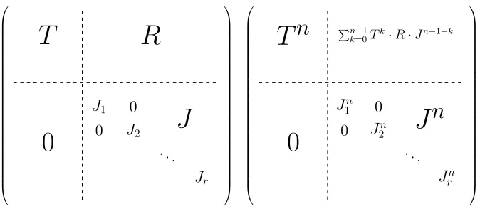
Jn 1 Jn 2 . .. Jn r 0 0Fig. 1.Decomposition ofP(on the left) and ofPn(on the right).
LetM ∈ SQ×Q(R), consider P = M|Q|!. It is easy to see that π(P) is idempotent. We decompose P as illustrated in Figure 1, by indexing states in the following way:
– first,π(P)-transient states,
In this decomposition, we have the following properties:
– for all m-transient states s ∈ Q, we have Pt m-transientT(s, t) < 1, so
||T||<1,
– the matricesJi are irreducible: for all statess, t ∈ Qcorresponding to the sameJi, we haveJi(s, t)>0.
The powerPnofP is represented in Figure 1.
This decomposition allows to treat separately the three blocks:
1. the blockTn: thanks to the observation above||T|| < 1, which combined with||Tn|| ≤ ||T||nimplies that(Tn)
n∈Nconverges to0exponentially fast, 2. the blockPnk=0−1Tk·R·Jn−1−k,
3. the blockJn: it is handled by Lemma 3.
We first focus on item 3., and show that the sequence(Jn)n∈N converges exponentially fast. Each blockJiis handled separately by the following lemma.
Lemma 3. (Powers of an irreducible stochastic matrix) LetJ ∈ SQ×Q(R)be irreducible: for all states s, t ∈ Q, we have J(s, t) > 0. Then the sequence
(Jn)n∈Nconverges exponentially fast to a matrixJ∞. Furthermore,J∞is irreducible.
This lemma is a classical result from Markov chain theory, sometimes called the Convergence Theorem; see for instance [8].
We now consider item 2., and show that the sequence (Pnk−=01Tk · R ·
Jn−1−k)n∈Nconverges exponentially fast. Observe that since||T||<1, the ma-trixI−T is invertible, whereIis the identity matrix with the same dimension asT. DenoteN = (I−T)−1, it is equal toPk≥0Tk. DenoteJ∞= limnJn, which exists thanks to Lemma 3.
We have:
||
n−1 X
k=0
Tk·R·Jn−1−k−N·R·J∞||
=||
n−1 X
k=0 h
Tk·R·Jn−1−k−J∞+Tk·R·J∞i−N ·R·J∞||
=||
n−1 X
k=0
Tk·R·Jn−1−k−J∞+
n−1 X
k=0
Tk−N !
·R·J∞||
≤ ||
n−1 X
k=0
Tk·R·Jn−1−k−J∞||+||
n−1 X
k=0
Tk−N !
We first consider the right summand:
||
n−1 X
k=0
Tk−N !
·R·J∞||
=||
X
k≥n Tk
·R·J∞||
≤ ||X
k≥n
Tk|| · ||R|| |{z}
≤1
· ||J∞|| | {z }
=1
=||Tn·N|| ≤ ||N|| · ||T||n.
The first equality follows from the fact thatPnk=0−1Tk−N =Pk≥nTk. Thus, this term converges exponentially fast to0.
We next consider the left summand. Thanks to Lemma 3, there exists a con-stantC >1such that for allp∈N, we have||Jp−J∞|| ≤C−p.
||
n−1 X
k=0
Tk·R·Jn−1−k−J∞||
≤
nX−1
k=0
||T||k· ||R|| |{z}
≤1
·||Jn−1−k−J∞||
≤
nX−1
k=0
||T||k· ||Jn−1−k−J∞||
=
bXn/2c
k=0
||T||k | {z }
≤1
·||Jn−1−k−J∞||+
n−1 X
k=bn/2c+1
||T||k· ||Jn−1−k−J∞||
| {z }
≤2
≤ C−
(bn/2c+1)−C−n
1−C + 2·
||T||bn/2c+1− ||T||n
1− ||T||
≤2· C−
(bn/2c+1)
1−C +
||T||bn/2c+1
1− ||T|| !
.
Thus, this term converges exponentially fast to0. We proved that(Pn)
n∈Nconverges exponentially fast to a matrixMω. We conclude the proof of Theorem 5 by observing that:
π(Mω)(s, t) =
(
1 ifπ(P)(s, t) = 1andtisπ(P)-recurrent,
Assume first thatπ(Mω)(s, t) = 1,i.e.Mω(s, t)>0. This already implies that t is π(P)-recurrent, looking at the decomposition of Pn. Since Mω = limnPn, it follows that fornlarge enough, we havePn(s, t) >0. The matrix π(P) is idempotent, so we have for all n ∈ Nthe equality π(Pn) = π(P), implying thatP(s, t)>0,i.e.π(P)(s, t) = 1.
Conversely, assume thatπ(P)(s, t) = 1andtisπ(P)-recurrent. Observe that for alln ∈ Nwe havePn+1(s, t) ≥ P(s, t)·Pn(t, t). Forn tending to infinity, this impliesMω(s, t) ≥P(s, t)·Mω(t, t). Note thatP(s, t) >0, and Mω(t, t) >0sincetisπ(P)-recurrent and thanks to Lemma 3. It follows that Mω(s, t)>0,i.e.π(Mω)(s, t) = 1.
4.5 Reformulating the Characterisation
For proof purposes, we give an equivalent presentation of the Markov Monoid throughω-expressions. Given a probabilistic automatonA, we define an inter-pretationh·iofω-expressions into Boolean matrices:
– haiisπ(φ(a)),
– hE1·E2iishE1i · hE2i,
– hEωiishEi], only defined ifhEiis idempotent.
Then the Markov Monoid ofAis{hEi |Eanω-expression}.
The following theorem is a reformulation of Theorem 1, using the pros-tochastic theory. It clearly implies Theorem 1: indeed, a polynomial prostochas-tic word induces a polynomial sequence, and vice-versa.
Theorem 6. (Characterisation of the Markov Monoid algorithm) The Markov Monoid algorithm answers “YES” on inputAif, and only if, there exists a poly-nomial prostochastic word accepted byA.
The proof relies on the notion of reification, used in the following proposi-tion, from which follows Theorem 6.
Definition 12. (Reification) LetAbe a probabilistic automaton.
A sequence(un)n∈N of words reifies a Boolean matrixm if for all states s, t∈Q, the sequence
PA(s−→un t)
n∈N
converges and:
m(s, t) = 1 ⇐⇒ lim
n PA(s un
−→t)>0.
Proposition 1. (Characterisation of the Markov Monoid algorithm) For every ω-expressionE, for everyφ:A→ SQ×Q(R), we have
π(φb(E)) =hEi.
– any sequence inducing the polynomial prostochastic wordEreifieshEi,
– the elementhEiof the Markov Monoid is a value1 witness if, and only if, the polynomial prostochastic wordEis accepted byA.
Proof. We prove the first part of Proposition 1 by induction on theω-expression E, which essentially amounts to gather the results from Section 4.
The base case ofa∈Ais clear.
The product case:letE =E1·E2, andφ:A→ SQ×Q(R).
By definition E = E1 ·E2, so φb(E) = φb(E1) ·φb(E2) because φbis a morphism, andπ(φb(E)) = π(φb(E1))·π(φb(E2)). Also by definition, we have
hEi=hE1i · hE2i, soπ(φb(E1·E2)) =hE1·E2i.
The iteration case:letE =Fω, andφ:A→ SQ×Q(R).
By definition,E=Fω, soφb(E) =φb(Fω), which is equal toφb(F)ωthanks to Lemma 2. Now,π(φb(F)ω) =π(φb(F))] thanks to Theorem 5. By induction hypothesis,π(φb(F)) =hFi, soπ(φb(Fω)) =hFωi.
We prove the second part. Consider a sequenceuinducing the polynomial prostochastic wordE. Thanks to the first item,π(φb(E)) = hEi, implying that π(limφ(u)) =hEi, which means thatureifiesE.
We prove the third part.
Assume thathEiis a value1witness,i.e.for all statest∈Q, ifhEi(q0, t) =
1, then t ∈ F. So fort /∈ F, we have limφ(u)(q0, t) = 0. Since we have
limφ(u)(q0, Q) = 1, it follows thatlimφ(u)(q0, F) = 1, soφb(E)(q0, F) = 1, i.e.the polynomial prostochastic wordEis accepted byA.
Conversely, assume that the polynomial prostochastic wordE is accepted byA. Since it is induced byu, it follows thatlimφ(u)(q0, F) = 1. Consider a statet∈Qsuch thathEi(q0, t) = 1. It follows thatπ(limφ(u))(q0, t) = 1, so
limφ(u)(q0, t) >0. Sincelimφ(u)(q0, F) = 1, this implies thatt∈F, hence
hEiis a value1witness.
5 Towards an Optimality Argument
In this section, we build on the characterisation obtained above to argue that the Markov Monoid algorithm is in some sense optimal.
5.1 Undecidability of the Two-Tier Value 1 Problem
Theorem 7. (Undecidability of the two-tier value 1 problem) The following problem is undecidable: given a probabilistic automatonA, determine whether there exist two finite wordsu, vsuch thatlimnPA((u·vn)2
n
p0
q0, L
A
F
qF
q0, R
A
F
⊥
check,1 2
check
∗
end end
check,1 2
check
∗
end
[image:21.612.161.460.129.262.2]end
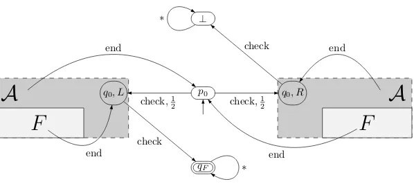
Fig. 2.Reduction.
The two-tier value1 problem seems easier than the value 1 problem as it restricts the set of sequences of finite words to very simple sequences. We call such sequences two-tier, because they exhibit two different behaviours: the word vis repeated a linear number of times, namelyn, while the wordu·vnis repeated an exponential number of times, namely2n.
The proof is obtained using the same reduction as for the undecidability of the value1problem, from [7], with a refined analysis.
Proof. We construct a reduction from the emptiness problem for probabilistic automata to the two-tier value1problem. For technical reasons, we will assume that the probabilistic automata have transition probabilities0,12, or1.
LetAbe a probabilistic automaton. We construct a probabilistic automaton
Bsuch that the following holds:
there exists a finite wordwsuch thatPA(w)> 12 if, and only if, there exist two finite wordsu, vsuch thatlimnPB((u·vn)2
n
) = 1.
The emptiness problem for probabilistic automata has been shown undecidable in [9]. We refer to [7] for a simple proof of this result.
Without loss of generality we assume that the initial stateq0 ofAhas no ingoing transitions.
The alphabet ofBisB =A] {check,end}, its set of states isQB =Q×
the only final state isqF. We describeφ0as a functionφ0 :QB×B → D(QB):
φ0(p0,check) = 12·(q0, L) +12 ·(q0, R)
φ0((q, d), a) = (φ(q, a), d)fora∈Aandd∈ {L, R}
φ0((q0, L),check) =qF
φ0((q, L),end) =q0ifq∈F φ0((q, L),end) =p0ifq /∈F φ0((q0, R),check) =⊥
φ0((q, R),end) =p0ifq ∈F φ0((q, R),end) =q0ifq /∈F φ0(qF,∗) =qF
where as a convention, if a transition is not defined, it leads to⊥.
Assume that there exists a finite word wsuch that PA(w) > 12, then we claim thatlimnPB((check·(w·end)n)2
n
) = 1. Denotex=PA(w). We have
PA(p0
check·(w·end)n
−−−−−−−−→(q0, L)) =
1 2·x
n,
and
PA(p0
check·(w·end)n
−−−−−−−−→(q0, R)) =
1
2 ·(1−x)
n.
We fix an integerNand analyse the action of reading(check·(w·end)n)N: there areN “rounds”, each of them corresponding to reading check·(w·end)n
from p0. In a round, there are three outcomes: winning (that is, remaining in
(q0, L)) with probabilitypn= 21 ·xn, losing (that is, remaining in(q0, R)) with probabilityqn = 12 ·(1−x)n, or going to the next round (that is, reachingp0) with probability1−(pn+qn). If a round is won or lost, then the next check leads to an accepting or rejecting sink; otherwise it goes on to the next round, forN rounds. Hence:
PA((check·(w·end)n)N)
=
NX−1
i=1
(1−(pn+qn))i−1·pn
=pn·
1−(1−(pn+qn))N−1
1−(1−(pn+qn))
= 1 1 +qn
pn
· 1−(1−(pn+qn))N−1
First, qn
pn = (
1−x
DenoteN =f(n)and consider the sequence((1−(pn+qn))N−1)n∈N; if
(f(n)·xn)n∈Nconverges to∞, then the above sequence converges to0. Since x > 12, this holds for f(n) = 2n. It follows that the acceptance probability converges to1. Consequently:
lim
n PA((check·(w·end) n)2n
) = 1.
Conversely, assume that for all finite wordsw, we havePA(w) ≤ 12. We claim that every finite word inB∗is accepted byBwith probability at most 12. First of all, using simple observations we restrict ourselves to words of the form
w=check·w1·end·w2·end· · · wn·end·w0,
withwi ∈A∗andw0 ∈B∗. SincePA(wi)≤ 12 for everyi, it follows that inB, after reading the last letter end inwbeforew0, the probability to be in(q0, L)is smaller or equal than the probability to be in(q0, R). This implies the claim. It follows that the value ofBis not1, and in particular for two finite words u, v, we havelimnPB((u·vn)2
n
)<1.
Note that the proof actually shows that one can replace in the statement of Theorem 7 the value2nbyf(n)for any functionf such thatf(n)≥2n.
5.2 Combining the Two Results
It was shown in [4] that the Markov Monoid algorithm subsumes all previous known algorithms to solve the value 1problem. Indeed, it was proved that it is correct for the subclass of leaktight automata, and that the class of leaktight automata strictly contains all subclasses for which the value1problem has been shown to be decidable.
At this point, the Markov Monoid algorithm is the best algorithmso far. But can we go further? If we cannot, then what is an optimality argument? It consists in constructing a maximal subclass of probabilistic automata for which the problem is decidable. We can reverse the point of view, and equivalently construct an optimal algorithm,i.e.an algorithm that correctly solves a subset of the instances, such that no algorithm correctly solves a superset of these in-stances. However, it is clear that no such strong statement holds, as one can always from any algorithm obtain a better algorithm by precomputing finitely many instances.
Polynomial Prostochastic Two-tier
Sequences
Markov Monoid algorithm
Undecidable
ε a b aaab babb aωP bωP
(aωPb)ωP (baωP)ωP
(abωP)ωPaωPb (a(ba)n)2n
(abn)2n
[image:24.612.150.469.125.295.2](ban)2n
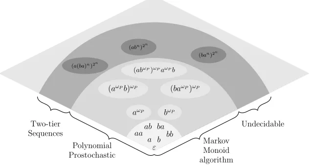
Fig. 3.Optimality of the Markov Monoid algorithm.
and of the undecidability of the two-tier value1problem from Subsection 5.1 supports the claim that the Markov Monoid algorithm isin some senseoptimal:
– The characterisation says that the Markov Monoid algorithm captures ex-actly all polynomial behaviours.
– The undecidability result says that the undecidability of the value1problem arises when polynomial and exponential behaviours are combined.
So, the Markov Monoid algorithm is optimal in the sense that it captures alarge set of behaviours, namely polynomial behaviours, and that no algorithm can capture both polynomial and exponential behaviours.
References
1. Jorge Almeida. Profinite semigroups and applications.Structural Theory of Automata, Semi-groups, and Universal Algebra, 207:1–45, 2005.
2. Krishnendu Chatterjee and Mathieu Tracol. Decidable problems for probabilistic automata on infinite words. InLICS, pages 185–194, 2012.
3. Nathanaël Fijalkow. Characterisation of an algebraic algorithm for probabilistic automata. InSTACS, pages 34:1–34:13, 2016.
4. Nathanaël Fijalkow, Hugo Gimbert, Edon Kelmendi, and Youssouf Oualhadj. Deciding the value 1 problem for probabilistic leaktight automata.Logical Methods in Computer Science, 11(1), 2015.
5. Nathanaël Fijalkow, Hugo Gimbert, and Youssouf Oualhadj. Deciding the value 1 problem for probabilistic leaktight automata. InLICS, pages 295–304, 2012.
7. Hugo Gimbert and Youssouf Oualhadj. Probabilistic automata on finite words: Decidable and undecidable problems. InICALP (2), pages 527–538, 2010.
8. David A. Levin, Yuval Peres, and Elizabeth L. Wilmer. Markov Chains and Mixing Times. American Mathematical Society, 2008.
9. Azaria Paz.Introduction to Probabilistic Automata. Academic Press, 1971. 10. Jean-Éric Pin. Profinite methods in automata theory. InSTACS, pages 31–50, 2009. 11. Michael O. Rabin. Probabilistic automata.Information and Control, 6(3):230–245, 1963. 12. Szymon Toru´nczyk.Languages of Profinite Words and the Limitedness Problem. PhD thesis,