Enhancing spectral unmixing by considering the point spread function effect

Enhancing spectral unmixing by considering the point spread function effect

Qunming Wang, Wenzhong Shi, Peter M. Atkinson

PII: S2211-6753(17)30324-X

DOI: https://doi.org/10.1016/j.spasta.2018.03.003

Reference: SPASTA 286 To appear in: Spatial Statistics

Received date : 8 December 2017 Accepted date : 13 March 2018

Please cite this article as: Wang Q., Shi W., Atkinson P.M., Enhancing spectral unmixing by considering the point spread function effect.Spatial Statistics(2018),

https://doi.org/10.1016/j.spasta.2018.03.003

Enhancing spectral unmixing by considering the point spread

1

function effect

2 3

Qunming Wang a,b,*, Wenzhong Shi c, Peter M. Atkinson a,d,e,f

4 5

a _{Lancaster Environment Centre, Lancaster University, Lancaster LA1 4YQ, UK}

6

b _{Centre for Ecology & Hydrology, Lancaster LA1 4YQ, UK}

7

c _{Department of Land Surveying and Geo-Informatics, The Hong Kong Polytechnic University, Kowloon, Hong Kong}

8

d _{Geography and Environment, University of Southampton, Highfield, Southampton SO17 1BJ, UK}

9

e _{School of Geography, Archaeology and Palaeoecology, Queen's University Belfast, BT7 1NN, Northern Ireland, UK}

10

f _{State Key Laboratory of Resources and Environmental Information System, Institute of Geographical Sciences and}

11

Natural Resources Research, Chinese Academy of Sciences, Beijing 100101, China 12

*Corresponding author. E-mail: [email protected] 13

14

Abstract: The point spread function (PSF) effect exists ubiquitously in real remotely sensed data 15

and such that the observed pixel signal is not only determined by the land cover within its own

16

spatial coverage but also by that within neighboring pixels. The PSF, thus, imposes a fundamental

17

limit on the amount of information captured in remotely sensed images and it introduces great

18

uncertainty in the widely applied, inverse goal of spectral unmxing. Until now, spectral unmixing

19

has erroneously been performed by assuming that the pixel signal is affected only by the land cover

20

within the pixel, that is, ignoring the PSF. In this paper, a new method is proposed to account for

21

the PSF effect within spectral unmxing to produce more accurate predictions of land cover

22

proportions. Based on the mechanism of the PSF effect, the mathematical relation between the

23

coarse proportion and sub-pixel proportions in a local window was deduced. Area-to-point kriging

24

(ATPK) was then proposed to find a solution for the inverse prediction problem of estimating the

25

sub-pixel proportions from the original coarse proportions. The sub-pixel proportions were finally 26

upscaled using an ideal square wave response to produce the enhanced proportions. The

27

effectiveness of the proposed method was demonstrated using two datasets. The proposed method

28

has great potential for wide application since spectral unmixing is an extremely common approach

29

in remote sensing.

30 31

Keywords: Land cover, Spectral unmixing, Soft classification, Point spread function (PSF), 32

Area-to-point-kriging (ATPK).

33 34 35

1. Introduction 36

37

Mixed pixels exist unaviodably in remotely sensed images. Mixed pixels cover more than one

38

land cover class such that the observed spectrum is a composite of the individual spectra for the

39

constituent land cover classes (also termed endmembers). Spectral unmixing is the goal of

40

predicting the areal proportions of the land cover classes within mixed pixels and it has been

41

investigated over two decades. It is beyond the scope of this paper to review explicitly the existing

42

methods for spectral unmixing, but several reviews exist (Bioucas-Dias et al., 2012; Quintano et al.,

43

2012). The linear spectral mixture model (LSMM) (Heinz & Chang, 2001; Keshava & Mustard,

44

2002) underpins the development of most of the existing spectral unmixing methods, with benefits

45

including its clear physical interpretation and mathematical simplicity. LSMM assumes that the

46

spectrum of a mixed pixel is a linear weighted sum of the endmembers.

48 49 50 51 52 53 54 55 56 57 58 59 60 61 62 63 64 65 66 67 68 69 70 71 72 73 74 75 76 77 78 79 80 81 The p mainly b resampl function Radoux of contri pixels (T on the a Fig. 1 sh and quan in Fig. 1 brighten bright ob In the id between proporti however Therefor unmixin

0 0

0 0

0 0

0 0

0 0

0 0

0 0

0

Fig. 1. An resolution of 56 by 5 (c) The 7 deviation and (c). (e boundary

It is o proporti pixels o importan

point spread by the optics

ing (Huang n (i.e., in bot et al., 2016 ibutions from Townshend amount of in hows an ex ntitative eva 1(c) are obv n dark objec bjects (e.g., deal coarse p n different la

ions whose r, the width re, the PSF ng.

(a)

.020 0.143 0 .143 1

.143 1

.143 1

.143 1

.143 1

.061 0.429 0

0 0

n example to n image of the 56 pixels). (b) m coarse spa is half of the c e) and (f) are th cells of the ob

of great inte ions in spect n the center nt in spectr

d function (P s of the instr g et al., 200 th the across

). Due to the m not only w

et al., 2000 nformation t ample illust aluation sho viously diffe cts (e.g., inc decrease th proportion im

and cover c width is on h of coarse b F can introd

(e)

0.143 0.041

1 0.286

1 0.286

1 0.286

1 0.286

1 0.286 0.429 0.122

0 0

illustrate the rectangle targ The ideal 7 m atial resolution coarse pixel si he correspond bject).

erest to deve tral unmixin

r pixel and ral unmixing

PSF) effect rument, the 02; Schowen

s-track and e PSF effect within the sp 0; Van der M that remote trating the P ows that wh

erent from t crease the a he actual pro mages, prod classes on th

nly one coa boundary c duce great u

(b) 0 0 0 0 0 0 0 0 0 0 0 0 0 0 0 0

PSF effect on get (with target m coarse spatial n proportion i ize). (d) The re ding matrices o

elop method ng. The meth eliminate it g and vario

exists ubiqu detector and ngerdt, 199 along-track t, the signal patial cover Meer, 2012) sensing ima PSF effect o en affected the actual c actual propo

oportion of duced with a he ground a arse pixel, a an be large uncertainty

0 0.

0 0.

0 0.

0 0.

0 0.

0 0.

0 0.

0

n observed lan t in pure white l resolution pr image observe elation betwee of the proporti

ds to consid hod needs to t. It is wide ous methods

uitously in r d electronic 97). The PS directions) attributed t rage of the p . Such an ef ages can con on observed

by the PSF oarse propo ortion of ze

one to a sm a square wav always resul as shown in er than one

in proporti

(c)

001 0.056 0 002 0.213 0 002 0.236 0 002 0.236 0 002 0.236 0 002 0.229 0 001 0.105 0

0 0.003 0

nd cover prop e and backgrou roportion imag ed using a sen en the ideal and

on images in (

der the PSF o consider th ely acknowl

s have been

remotely sen cs, atmosphe F is usually

(Campagno to a given pi pixel, but als ffect leads t ntain (Mans d coarse pro , the observ ortions in Fi ero to a larg maller value) ve response, lts in a boun n Fig. 1(e).

coarse pixe ion estimati

(f)

0.213 0.223 0 0.815 0.852 0 0.903 0.944 0 0.903 0.944 0 0.903 0.944 0 0.876 0.916 0 0.400 0.418 0 0.013 0.014 0

portions. (a) T und in pure bla ge for the targe nsor with a Ga d observed 7 m (b) and (c) (the

effect to pr he impact of ledged that n developed

nsed data. It eric effects,

y expressed olo & Monta ixel is a wei so that for ne to a fundam

slow & Nix oportions. B ved coarse p ig. 1(b). Th ger value) a ) (Huang et the original ndary of int Because of el, shown in

ion based o

(d) 0.079 0.001 0.301 0.006 0.333 0.006 0.333 0.006 0.333 0.006 0.323 0.006 0.148 0.003 0.005 0.001 The simulated ack) on the gro et (image of 8

aussian PSF ( m proportion i e blue values r

roduce mor f spatially ne

spatial info d on this ba

0 0. 0 0.5 1 Actual pro P red ic ted p ro p or ti o n s

t is caused and image d as a 2-D ano, 2014; ighted sum eighboring mental limit xon, 2002). Both visual roportions he PSF can and darken al., 2002). l boundary termediate f the PSF, n Fig. 1(f). on spectral 0 0 0 0 0 0 0 0 0 0 0 0 0 0 0 0

d 1 m spatial ound (image

by 8 pixels). (the standard images in (b) represent the

re accurate eighboring rmation is sis. Shi &

Wang (2014) provided a comprehensive review of existing methods that incorporate spatial

82

information in spectral unmixing. These methods mainly incorporate spatial information in

83

endmember extraction, selection of endmember combinations and abundance estimation. However,

84

very few methods consider the PSF effect from the viewpoint of the physical mechanism. That is,

85

very few studies focus on how the neighboring pixels affect the center coarse pixel based on the

86

PSF effect and consider how to eliminate such an effect. Townshend et al. (2000) and Huang et al.

87

(2002) proposed a deconvolution method to reduce the influence of the PSF in proportion

88

estimation. This method quantifies the contributions from neighbors on the basis of coarse

89

pixel-level information and treats all sub-pixels locations in a coarse neighbor equally. However,

90

different sub-pixel locations in the coarse neighbor have different spatial distances to the center

91

coarse pixel and can have different influences on the center coarse proportion. Therefore, it is

92

necessary to develop methods to consider the impact of neighbors at the sub-pixel scale.

93

In this paper, we propose a new method to account for the PSF effect in spectral unmixing and

94

produce more accurate proportion predictions. The method predicts the land cover proportions at a

95

finer spatial resolution inversely from the original coarse proportions before predicting the

96

enhanced proportions (i.e., the final predictions at the same coarse spatial resolution with the

97

original proportions, but the PSF effect is reduced). Section 2 first introduces the mechanism of the

98

PSF effect on spectral unmixing and deduces the mathematical relation between the coarse

99

proportions and sub-pixel proportions of both the coarse center pixel and its coarse neighbors.

100

Based on the deduced relation, the area-to-point kriging (ATPK) method is then introduced to

101

predict the sub-pixel proportions from the original coarse proportions. For validation of the method,

102

Section 3 provides and analyzes the experimental results for two datasets. The method is further

103

discussed with several open issues in Section 4. A conclusion is provided in Section 5.

104 105 106

2. Methods 107

108

2.1. The effect of the PSF on spectral unmixing 109

110

Suppose S_V is the spectrum of coarse pixel V, R( )k is the spectrum of class endmember k (k=1, 111

2, …, K, where K is the number of land cover classes), and F kV( ) is the proportion of class k within 112

coarse pixel V. Based on the classical linear spectral mixture model, the spectrum of a coarse pixel 113

is a linearly weighted spectra of endmembers, where the weights are class proportions within the

114

coarse pixel:

115

1

( ) ( )

K

V V

k

k F k







S R . (1) 116

Due to the PSF effect, the spectrum of coarse pixel V can be considered as a convolution of the 117

spectra of sub-pixels

118

V  vhV

S S (2)

119

in which S_v is the spectrum of sub-pixel v, * is the convolution operator and hV is the PSF. The 120

spectrum of sub-pixel v can be characterized as 121

1

( ) ( )

K

v v

k

k F k







S R (3) 122

where F kv( ) is the proportion of class k in sub-pixel v. Substituting Eq. (3) into Eq. (2), we have





1 1

( ) ( ) = ( ) ( )

K K

V v V v V

k k

k F k h k F k h

 

 

_{ } 







S R R . (4)

124

Comparing Eqs. (1) and (4), we can conclude

125

( ) ( )

V v V

F k F k h . (5)

126

This means that the predicted coarse proportion (e.g., based on the classical linear spectral mixture

127

model) within each coarse pixel, F k_V( ), is a convolution of the sub-pixel proportions.

128

In theory, the true (i.e., ideal) coarse proportion (denoted as T k_V( )) is identified as the average of

129

all sub-pixel class proportions ( )F k_v within the center coarse pixel. That is, for ( )T kV , the PSF 130

(denoted as h_V) is an ideal square wave filter 131

1

, if ( , ) ( , ) ( , )

0, otherwise

V

i j V i j h i j   _ 



 . (6)

132

In Eq. (6),  is the areal ratio between the pixel sizes of V and v, (i, j) is the spatial location of the 133

sub-pixel and V i j( , ) is the spatial coverage of the coarse pixel V in which each sub-pixel located 134

at (i, j) falls. Eq. (6) means that based on the square wave filter, only the sub-pixels within the 135

coarse pixel V will affect the coarse pixel and, moreover, all of them will exert the same effect. The 136

relation between ( )T k_V and ( )F k_v is expressed as 137

( ) ( )

V v V

T k  F k h . (7) 138

In reality, the PSF h_V in Eq. (5) is different to the ideal square wave PSF h_V in Eq. (7) (i.e., 139

V V

h h ). The spatial coverage of h_V is generally larger than a coarse pixel extent and different

140

sub-pixels may have different effects on the coarse pixel. For example, the PSF is often assumed to

141

be a Gaussian filter (Huang et al., 2002; Townshend et al., 2000; Van der Meer, 2012)

142

2 2

2 2

1

exp , if ( , ) ( , )

( , ) _{2 2}

0, otherwise

V

i j

i j V i j

h i j _{ }

    

 __{ }  

  _{  }

  

(8)

143

where  is the standard deviation (i.e., the width of the Gaussian PSF) and V i j( , ) is the spatial

144

coverage of the local window centered at coarse pixel V ( ( , )V i j is larger than V i j( , ) in Eq. (6)). 145

Based on the Gaussian PSF, F kV( ) is actually a convolution of the sub-pixel proportions in the

146

local window centered at the coarse pixel V, rather than being restricted to only the sub-pixel 147

proportions within the coarse pixel V. Moreover, the sub-pixels with different spatial distances to 148

the center coarse pixel will exert different effects on it. Thus, due to the PSF effect, F k_V( ) is

149

actually contaminated by the sub-pixels surrounding the coarse pixel V. 150

Evidently, the difference between h_V and h_V makes the predicted coarse proportion F k_V( )

151

different to the ideal coarse proportion ( )T k_V . The spectral unmixing predictions ( )F k_V can, 152

however, be enhanced by considering the PSF effect. To produce more accurate coarse proportions

153

(i.e., predictions that are as close to ( )T k_V as possible), the sub-pixel proportions ( )F k_v need to be 154

predicted. As seen from Eq. (5), just as F k_V( ) is obtained from spectral unmixing, F k_v( ) can be

155

157

2.2. Area-to-point kriging (ATPK) for enhancing the original coarse proportions 158

159

The key in the inverse prediction problem of estimating a sub-pixel proportion F kv( ) from

160

coarse proportion ( )F k_V is to account for the PSF h_V which introduces the contributions of 161

neighboring pixels to the coarse proportion of center pixel V. This process involves downscaling. 162

ATPK is a powerful choice for downscaling, which can account for the PSF effect explicitly in the

163

scale transformation (Kyriakidis, 2004). In this paper, it is used to downscale the coarse

164

proportions to the finer spatial resolution proportions F k_v( ).

165

Based on ATPK, the sub-pixel proportion is calculated as a linear weighted sum of the

166

neighboring coarse proportions

167

1 1

ˆ ( ) ( ), s.t. 1

i

N N

v i V i

i i

F k F k 

 







168

in which _i is the weight for the ith coarse neighbor Vi and N is the number of neighbors. The N 169

weights are calculated according to a kriging matrix, where the semivariograms at different spatial

170

resolutions account for the PSF in scale transformation. Details on the kriging matrix and

171

semivariograms can be found in Wang et al. (2015, 2016a).

172

ATPK has the appealing advantage of honoring the coarse data perfectly. This means that when

173

the ATPK predictions F kˆ ( )_v are convolved with the PSF h_V , exactly the original coarse

174

proportions F k_V( ) are produced (Kyriakidis, 2004)

175

ˆ

( ) ( )

V v V

F k F k h . (10)

176

By comparing Eqs. (5) and (10), we can consider the ATPK predictions F kˆ ( )_v as a reliable

177

solution to the inverse prediction problem of estimating the sub-pixel proportions F k_v( ).

178

The final coarse proportion for class k is calculated as a convolution of ˆ ( )F kv with the ideal 179

square wave filter h_V 180

ˆ _{( )} ˆ _{( )}

V v V

T k  F k h . (11) 181

That is, for each coarse pixel, the final proportion for class k is predicted as the average of ˆ ( )F v_k 182

within it. Fig. 2 describes the process of predicting T k_V( ) from the original coarse proportion

183

( )

V F k . 184

ˆ ( )_v

F k

( )

V

F k

ˆ ( )_V

T k

ˆ ( )_{v V V}( )

F k h F k

ˆ _{( )} ˆ_{( )}

V v V

T k F k h 

185

Fig. 2. Flowchart of transforming the original coarse proportion F k_V( ) to T k_V( ).

The implementation of the proposed ATPK-based method that accounts for the PSF in spectral

188

unmixing is not affected by the specific form of PSF and the method is suitable for any PSF. Once 189

the PSF is known or predicted, it can be used readily in the method.

190 191 192

3. Experiments 193

194

The proposed method for considering the PSF effect in spectral unmixing was demonstrated

195

using two datasets, including a land cover map and a multispectral image. As the estimation of the

196

PSF of sensors remains open and the proposed method is suitable for any PSF, the coarse data

197

(coarse proportions or multispectral image) were synthesized by convolving the available fine

198

spatial resolution land cover map or multispectral image, using the widely acknowledged Gaussian

199

PSF in Eq. (8) (Huang et al., 2002; Townshend et al., 2000; Van der Meer, 2012). The width of the

200

PSF was set to half of the coarse pixel size. The strategy can help to avoid the uncertainty in PSF

201

estimation and concentrate solely on the performance of proportion prediction. Moreover, the

202

coarse proportions are known perfectly and can be used as reference data for evaluation.

203

The root mean square error (RMSE) and correlation coefficient (CC) were used for quantitative

204

evaluation between the proportion predictions and real proportions. To emphasize the increase in

205

accuracy of the predictions of the proposed method over the original ones contaminated by the PSF,

206

an index called the reduction in remaining error (RRE) (Wang et al., 2015) was also used. Details

207

on the calculation of RRE can be referred to Wang et al. (2015).

208 209

3.1. Experiment on the land cover map 210

211

A land cover map (with a spatial resolution of 0.6 m) covering an area in Bath, UK was used in

212

this experiment, as shown in Fig. 3. The map has a spatial size of 360 by 360 pixels. Four classes

213

were identified in the land cover map, including roads, trees, buildings and grass. The map was

214

degraded by a factor of 8 and a square wave PSF, generating four actual proportion images at a

215

spatial resolution of 4.8 m, as shown Fig. 4(a). Similarly, the four original coarse proportion

216

images produced by spectral unmixing were simulated using a factor of 8 and a Gaussian PSF (the

217

width of the PSF was set to 2.4 m), as shown Fig. 4(b).

218

Fig. 5(a) shows the scatter plots between the actual proportions and original proportions

219

contaminated by the PSF. A visual check of both Figs. 4 and 5 reveals that due to the PSF effect,

220

the original proportions are obviously different from the actual proportions. For example, some

221

actual proportions of 0 are inaccurately predicted as a larger value (for grass, the value can reach

222

0.3, as shown in Fig. 5(a)) and some actual proportions of 1 are inaccurately predicted as a much

223

smaller value (e.g., some of the trees proportions are incorrectly predicted as 0.7, see Fig. 5(a)). Fig.

224

4(c) shows the enhanced proportions produced using the proposed method that considers the PSF

225

effect. Compared with the original proportion images in Fig. 4(b), the enhanced proportion images

226

in Fig. 4(c) are visually closer to the reference in Fig. 4(a). For example, the enhanced proportion

227

images are clearly much brighter than the original proportion images. The scatter-plots between the

228

actual proportions and enhanced proportions accounting for the PSF are shown in Fig. 5(b).

229

Compared with Fig. 5(a), the distribution of points for all four classes in Fig. 5(b) is more compact

230

and closer to the line of y =x, suggesting that the enhanced proportions are closer to the actual 231

proportions.

234 235 236 237 238

239 240

241 242

243 244 245 246 247 248

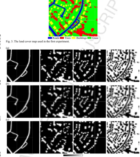
Fig. 3. Th (a)

(b)

(c)

Fig. 4. Th map with convolvin

he land cover m

he proportion i h an ideal wav

ng the 0.6 m l

map used in th

images for the ve square PSF and cover ma

he first experim

0 e land cover m

F and a degra ap with a Gaus

ment.

0 map. (a) Refere adation factor ssian PSF and

1

ence produced r of 8. (b) Or d a degradation

by convolvin riginal propor n factor of 8.

ng the the 0.6 m rtion images p (c) Enhanced

using the proposed method that considers the PSF effect in spectral unmixing. From left to right are the results for 249

roads, trees, buildings and grass. 250

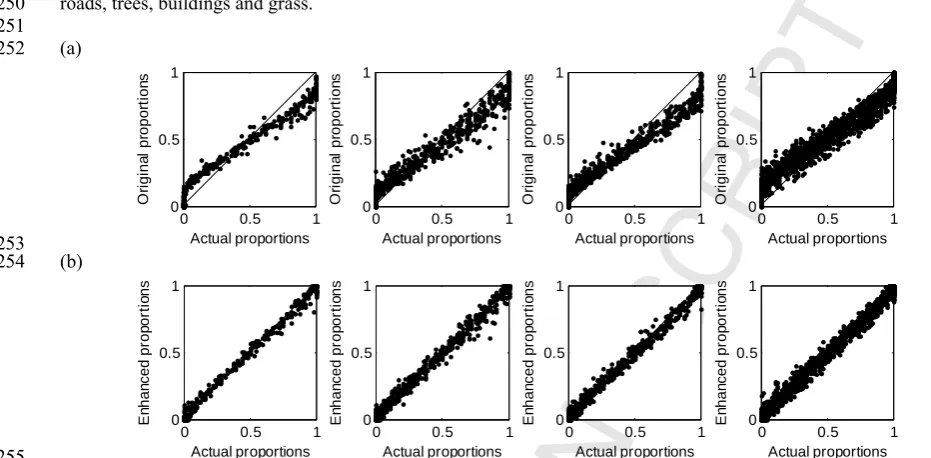
251 (a) 252

253 (b) 254

255

Fig. 5. (a) Relation between the actual proportions and original proportions in Fig. 4(b). (b) Relation between the actual 256

proportions and enhanced proportions in Fig. 4(c). From left to right are the results for roads, trees, buildings and grass. 257

258

Table 1 lists the accuracies of the proportions before and after considering the PSF effect. It is

259

seen that by considering the PSF effect, the enhanced proportions have larger CCs and smaller

260

RMSEs than the original proportions. More precisely, the RMSEs decrease by around 0.03, 0.04,

261

0.04 and 0.06 for roads, trees, buildings and grass, and the RREs are 69.55%, 61.11%., 65.14% and

262

63.53%. Correspondingly, the RREs for CCs of the four classes are 88.06%, 81.20%, 83.33% and

263

82.21%, revealing that the errors are greatly reduced by considering the PSF effect.

264 265

Table 1 Accuracy of the proportions for the land cover map 266

Roads Trees Buildings Grass

RMSE

Original 0.0440 0.0576 0.0591 0.0924 Enhanced 0.0134 0.0224 0.0206 0.0337

RRE 69.55% 61.11% 65.14% 63.53% CC

Original 0.9866 0.9867 0.9844 0.9792 Enhanced 0.9984 0.9975 0.9974 0.9963

RRE 88.06% 81.20% 83.33% 82.21% 267

The performance of the proposed method for different PSF width (i.e., 0.25, 0.5, 0.75 and 1) is

268

shown in Fig. 6. It is clear that the enhanced proportions have consistently larger CCs than the

269

original proportions for all three cases and all four land cover classes. Moreover, the accuracy gains

270

become larger when the width increases. For the width of 0.25, the CCs of original and enhanced

271

proportions are very close (both close to 1, with difference about 0.001), but the difference increase

272

to be larger than 0.04 for the width of 1. It is worth noting that the accuracies of both original and

273

enhanced proportions decrease as the width increases.

274 275 276 277 278

0 0.5 1 0

0.5 1

Actual proportions

O

ri

g

in

a

l pr

opor

ti

on

s

0 0.5 1 0

0.5 1

Actual proportions

O

ri

g

in

a

l pr

opor

ti

on

s

0 0.5 1 0

0.5 1

Actual proportions

O

ri

g

in

a

l pr

opor

ti

on

s

0 0.5 1 0

0.5 1

Actual proportions

O

ri

g

in

a

l pr

opor

ti

on

s

0 0.5 1 0

0.5 1

Actual proportions

E

n

ha

n

c

e

d

pr

op

or

ti

o

n

s

0 0.5 1 0

0.5 1

Actual proportions

E

n

ha

n

c

e

d

pr

op

or

ti

o

n

s

0 0.5 1 0

0.5 1

Actual proportions

E

n

ha

n

c

e

d

pr

op

or

ti

o

n

s

0 0.5 1 0

0.5 1

Actual proportions

E

n

ha

n

c

e

d

pr

op

or

ti

o

n

279

280 281 282

283 284 285 286 287 288 289 290 291 292 293 294 295 296 297 298 299 300 301 302 303 304

Fig. 6. Th pixel). (a)

3.2. Exp

To en multispe six-band acquired pixels an Province Referrin original six-band the mea degrade

The ta m multis the 30 m Fig. 8 sh

he CC of the or )-(d) are result

periment on

nsure the p ectral image d (bands 1-d in August nd covers fa e, China. T ng to the lan six-band 30 d 30 m mult an and varia

d with a fact ask of this e spectral ima m land cover hows the 24

CC

CC

riginal and enh ts for roads, tr

the multisp

perfect relia e was used -5 and 7) 3 t 2001, as sh

armland wit The correspo nd cover map 0 m Landsat tispectral im ance of the tor of 8 and experiment i age. The actu

r map in Fig 40 m actual

(a)

(c)

hanced propor ees, buildings

ectral imag

ability of t d in this exp

0 m Lands hown in Fig th four main onding man

p in Fig. 7(b t image wer mage was sy e classes. F

a Gaussian is to predict ual 240 m p g. 7(b) with proportions

σ

σ

rtions in relatio

and grass, res

ge

the referenc periment. S at-7 Enhan g. 7(a). The n land cover nually digiti b), the mean re calculated ynthesized b

inally, the PSF to crea t the 240 m roportions ( an ideal squ s, the origina

CC

CC

(

(

on to the width spectively.

ce (i.e., act Specifically, ced Thema e study area

r classes (m ized land co n and varian

d. Accordin based on the synthesized ate a 240 m m

coarse prop (i.e., referen uare wave P al proportio

(b)

(d)

h of the Gauss

tual propor , the image atic Mapper

has a spati marked as C1

over map is nce of each l ng to the land

e random no d 30 m mul multispectra portions from nce) were pro PSF and a de ons produced

σ

σ

ian PSF (in un

rtions), a sy e was create plus (ETM al size of 2 1–C4) in the

s shown in land cover c d cover in F ormal distrib ltispectral i al image, see m the synthe oduced by c egradation f d without co

nits of coarse

305 306 307 308 309 310 311

312 313 314 315 316 317 318

319 320

321 322

323

the PSF clear tha also sup consider 0.03, 0.0 and 52.2

Fig. 7. Th RGB). (b) C4). (c) 24 a degrada (a)

(b)

(c)

effect and at the enhan pported by th

ring the PSF 04, 0.03 and 27%, respec

he multispectra ) 30 m land co 40 m coarse im ation factor of

the enhanc nced proport he scatter-p F effect bas d 0.02, and ctively.

(a)

al image used over map prod mage produced

8.

ed proportio tions are clo plots in Fig. ed on the pr the RREs in

d in the second duced by draw d by degrading

ons produce oser to the re

9. The quan roposed me n terms of C

(b)

d experiment. wing manually g the synthesiz

ed using the eference than ntitative ass ethod, the R

CC for C1–C

(a) Original 3 from (a) (blue zed 30 m multi

e proposed n the origin sessment is RMSEs for C

C4 are 38.3

(c)

30 m multispe e, red, yellow ispectral imag

method. It al proportio shown in T C1–C4 are r 38%, 60.68%

ectral image (b and green rep e with a Gauss

is visually ons. This is able 2. By reduced by %, 76.92%

bands 432 as presents C1–

324 325 326 327 328 329 330 331 332 333 334 335 336 337 338 339 340 341 342 343 344 345 346 347 348 349 350 351 352 353 354

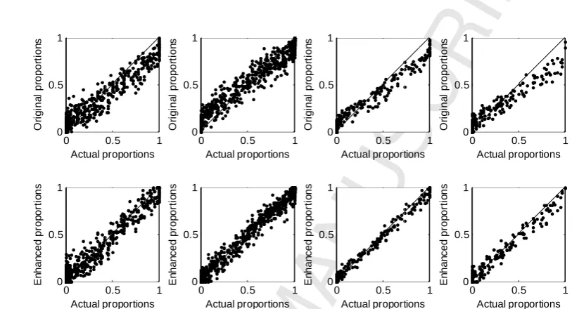
Fig. 8. Th map in Fig by spectra Enhanced are the res (a)

(b)

Fig. 9. (a) proportion results for 4. Discu After remote s climate c et al., 20 (Eckman (Weng e unmixin be enhan for enha example

he proportion i g. 7(b) with an al unmixing o d proportions u sults for C1–C

Relation betw ns and enhanc r C1–C4.

ussion

hard land co sensing, and change mon 008), precis nn et al., 2 et al., 2004 ng (indexed nced by con ancing the p e, the global

0 0 0 0.5 1 Actual p O ri g in a l p ropor ti on s 0 0 0 0.5 1 Actual p E n ha n c e d pr op or ti o n s

images for the n ideal square of the 240 m c using the propo C4.

ween the actua ed proportions

Table 2 A

RMSE O En CC O En over classifi d has been nitoring (Me sion agricult 2010), geolo 4). In the la

in Web of S nsidering the proportions l Vegetation 0.5 1 proportions O ri g in a l p ropor ti on s 0.5 1 proportions E n ha n c e d pr op or ti o n s 0 e multispectral

wave PSF and coarse multisp osed method t

l proportions a s in Fig. 8(c). F

ccuracy of the Original 0. nhanced 0. RRE 29 Original 0. nhanced 0. RRE 38 fication, spec applied wid elendez-Pas ture (Pachec ogical mapp ast five year Science). Th e PSF effect

is, thus, exp n Continuou 0 0.5 0 0.5 1 Actual prop 0 0.5 0 0.5 1 Actual prop 0 l image. (a) Re d a degradation pectral image that considers

and original pr From left to ri

e proportions f C1 C2 0873 0.09 0613 0.05 9.78% 43.1 9703 0.97 9817 0.99 8.38% 60.6 ctral unmixi dely in vari tor et al., 20 co and McN ping (Bedin rs, more tha he experime

through the pected to ha s Field (VC

1 portions 0 0.5 1 O ri g in a l p ropor ti on s 1 portions 0 0.5 1 E n ha n c e d pr op or ti o n s 1 eference produ n factor of 8. (

in Fig. 7(c), w the PSF effect

roportions in F ght are the res

for the multisp 2 C3 950 0.051 540 0.022 6% 55.71% 766 0.984 908 0.996 68% 76.92%

ing is one of ious domain 010), terrestr Nairn, 2010 ni, 2009), a an 1000 pa ntal results e proposed A

ave widespr CF) product h

0 0.5 0 5 1 Actual proport 0 0.5 0 5 1 Actual proport

uced by convo (b) Original pr without consi t in spectral un

Fig. 8(b). (b) R sults for C1-C4

pectral image C4 7 0.0529 9 0.0331 % 37.43% 4 0.9692 4 0.9853 % 52.27%

f the most co ns (Somers

rial ecosyste ), natural ha and urban e apers were p

reveal that s ATPK-based read applica has been gen

1 tions 0 0 0.5 1 A O ri g in a l p ropor ti on s 1 tions 0 0 0.5 1 A E n ha n c e d pr op or ti o n s

olving the 30 m roportion imag

dering the PS nmixing. From

Relation betwe 4. From left to

ommon app et al., 2011 em monitori azard risk a environment published o spectral unm d method. T ations in pra

nerated annu

0.5 Actual proportion

0.5 Actual proportion

m land cover ges produced SF effect. (c) m left to right

en the actual right are the

proaches in 1), such as

the Moderate Resolution Imaging Spectroradiometer (MODIS) since 2000, which contains the

355

percentage of vegetative cover within each MODIS pixel (DiMiceli et al., 2011). MODIS data have

356

also been used for crop area estimation based on spectral unmixing (Pan et al., 2012). The VCF

357

products and crop area estimation can be potentially enhanced by accounting for the PSF effect.

358

Sub-pixel mapping (Atkinson 1997; Wang et al., 2016b) has been developed for decades, which

359

is a post-processing analysis of spectral unmixing. It creates a thematic map at a finer spatial

360

resolution based on the spectral unmixing predictions as inputs. Specifically, under the proportion

361

coherence constraint and starting with the coarse proportions, sub-pixel mapping divides each

362

mixed pixel into sub-pixels and predicts their land cover class. When the PSF effect is considered

363

in the coarse proportions, more reliable inputs and proportion constraints can be provided for

364

sub-pixel mapping to create more accurate finer spatial resolution land cover maps.

365

According to the relation in Eq. (5), the proposed ATPK-based method can predict sub-pixel

366

proportions (i.e., a by-product) inversely from the coarse proportions. The by-product has a finer

367

spatial resolution than the original proportions and is also expected to have great application value.

368

For example, Gu et al. (2008) produced finer spatial resolution proportion images from input

369

coarse proportion images and the results (e.g., Fig. 10(f) in Gu et al., 2008) showed that aircraft can

370

be observed more clearly from the sub-pixel proportion images. For sub-pixel mapping, the

371

by-product can be hardened to create a finer spatial resolution land cover map, under the proportion

372

coherence constraint from the enhanced coarse proportions. This is also the core idea of the

373

recently developed soft-then-hard sub-pixel mapping algorithm (Wang et al., 2014), which predicts

374

sub-pixel proportion images first and then hardens them to land cover maps. The by-product, along

375

with the enhanced proportions, opens new avenues for future research.

376

In our previous research, the PSF effect was considered directly in the post SPM process (Wang

377

and Atkinson, 2017) to produce more accurate sub-pixel resolution land cover maps. Alternatively,

378

this paper aims to produce more accurate coarse proportions. As discussed above, the coarse

379

proportions have more general applications, including not only in the post SPM process, but also in

380

practical applications such as in large scale crop area and VCF estimation. The by-product of

381

sub-pixel proportions also imposes extra value. It would be interesting to conduct a comparison for

382

SPM predictions based on the method in Wang and Atkinson (2017) and the enhanced coarse

383

proportions produced using the proposed method in this paper.

384

The PSF width (i.e., standard deviation of the Gaussian PSF in this paper) determines how

385

greatly the observed pixel signal is affected by its neighboring pixels. It is a crucial factor affecting

386

the accuracy of spectral unmixing predictions. When the width increases, more neighbors

387

contaminate the center pixel and the uncertainty in predicting the proportions increases as a result,

388

and vice versa. Thus, the accuracy of the proportions (either original or enhanced) decreases as the 389

width increases, as reported in Fig. 6. It is worth noting that in Fig. 6, the accuracies of both original

390

and enhanced proportions for the width of 0.25 are nearly the same and both values are close to the

391

ideal value. This reveals that a very narrow PSF (e.g., less than 0.5 pixel) on a discrete grid (i.e.,

392

pixel) has little effect. It should be noted that each senor has its own PSF width. For example, based

393

on the assumption of the Gaussian PSF, Radoux et al. (2016) found that the width for the Landsat 8

394

red band is 0.72 pixel and ranges from 0.71 to 0.94 pixel for the Sentinel-2 bands. The consistently

395

greater accuracy of the proposed method for different widths suggests its great application value

396

for different sensors.

397

In this paper, a Gaussian PSF was assumed for convenience in the experimental validation. It

398

should be noted that the PSF may not be the Gaussian filter in reality, especially for sensors with a

399

scanning mirror which will ensure that the shape has a directional component (Tan et al., 2006).

400

However, this paper aims to find a solution to account for the PSF effect to enhance spectral

unmixing predictions. We did not focus on the specific form of the PSF (e.g., specific form of the

402

function and related parameters), as the proposed method is suitable for any PSF. In practice, once

403

the PSF is available, it can be used readily in the proposed ATPK-based method.

404

It is assumed that the endmembers are scale-free and that the same endmembers can be

405

considered for the coarse and fine spatial resolution spectra in Eqs. (1) and (3). This assumption is

406

more reliable when the landscapes are homogeneous or the intra-class spectra variation is small,

407

such that slight differences exist between the endmembers at different spatial resolutions. However,

408

intra-class spectral variation is a common problem in spectral unmixing that remains open

409

(Drumetz et al., 2016; Somers et al., 2011). It would be worthwhile to investigate the relation

410

between the endmembers at different spatial resolutions, or to consider endmember extraction in a

411

local window and the use of multiple endmembers to characterize each land cover class.

412

The proposed ATPK-based method is shown to be effective in considering the PSF effect, based

413

on the assumption that the ATPK predictions F kˆ ( )_v are a reliable solution to the inverse prediction

414

problem of estimating sub-pixel proportion ( )F k_v from F k_V( ). However, this inverse prediction 415

problem is ill-posed, and multiple solutions may meet the coherence constraint in Eq. (10). In

416

future research, it would be interesting to design an appropriate model to incorporate additional

417

information (e.g., prior spatial structure information for each land cover class at the fine spatial

418

resolution) into the ATPK method to reduce the solution space and produce more reliable sub-pixel

419

proportions.

420 421 422

5. Conclusion 423

424

A new method was proposed for considering the PSF in spectral unmixing and increasing the

425

accuracy of land cover proportion predictions. Based on the ubiquitous existence of the PSF effect

426

in real remotely sensed images, spectral unmixing predictions are made as a convolution of the

427

sub-pixel proportions of both the coarse center pixel and coarse neighbors. ATPK is proposed to

428

predict the sub-pixel proportions inversely from the coarse proportions and the sub-pixel

429

proportions are then convolved with the ideal square wave PSF to produce the final predictions.

430

The experimental results on two datasets suggest that the proposed method provides a satisfactory

431

solution for reducing the PSF effect in spectral unmixing.

432 433 434

Acknowledgment 435

436

This work was supported in part by the Research Grants Council of Hong Kong under Grant

437

PolyU 15223015 and in part by the National Natural Science Foundation of China under Grant

438

41331175.

439 440 441

References 442

443

Atkinson, P. M. (1997). Mapping sub-pixel boundaries from remotely sensed images. Innov. GIS 444

4, 166–180. 445

Bedini, E., van der Meer, F., van Ruitenbeek, F. (2009). Use of HyMap imaging spectrometer data

446

to map mineralogy in the Rodalquilar caldera, southeast Spain. International Journal of 447

Bioucas-Dias, J. M., Plaza, A., Dobigeon, N., Parente, M., Du, Q., Gader, P., Chanussot, J. (2012).

449

Hyperspectral unmixing overview: Geometrical, statistical and sparse regression-based

450

approaches. IEEE Journal of Selected Topics in Applied Earth Observations and Remote 451

Sensing, 5, 354–379. 452

Campagnolo, M. L., & Montano, E. L. (2014). Estimation of effective resolution for daily MODIS

453

gridded surface reflectance products. IEEE Transactions on Geoscience and Remote Sensing, 454

52, 5622–5632.

455

DiMiceli, C., Carroll, M., Sohlberg, R., et al. (2011). Annual global automated MODIS vegetation

456

continuous fields (MOD44B) at 250 m spatial resolution for data years beginning day 65,

457

2000-2010, collection 5 percent tree cover. USA: University of Maryland, College Park, MD. 458

Drumetz, L., Chanussot, J., Jutten, C., 2016. Variability of the endmembers in spectral unmixing:

459

recent advances. 8th Workshop on Hyperspectral Image and Signal Processing: Evolution in 460

Remote Sensing (WHISPERS 2016), Los Angeles, United States. 461

Eckmann, T. C., Still, C. J., Roberts, D.A., Michaelsen, J. C. (2010). Variations in subpixel fire

462

properties with season and land cover in Southern Africa. Earth Interactions, 14(6). 463

Gu, Y., Zhang, Y., Zhang, J. (2008). Integration of spatial–spectral information for resolution

464

enhancement in hyperspectral images. IEEE Transactions on Geoscience and Remote Sensing, 465

46, 1347–1358.

466

Heinz, D. C., Chang, C. I. (2001). Fully constrained least squares linear spectral mixture analysis

467

method for material quantification in hyperspectral imagery. IEEE Transactions on 468

Geoscience and Remote Sensing, 39, 529–545. 469

Hestir, E. L., Khanna, S., Andrew, M. E., Santos, M. J., Viers, J. H., Greenberg, J. A., et al. (2008).

470

Identification of invasive vegetation using hyperspectral remote sensing in the California Delta

471

ecosystem. Remote Sensing of Environment, 112, 4034−4047. 472

Huang, C., Townshend, R.G., Liang, S., Kalluri, S. N. V., DeFries, R. S. (2002). Impact of sensor’s

473

point spread function on land cover characterization: assessment and deconvolution. Remote 474

Sensing of Environment, 80, 203–212. 475

Keshava, N., Mustard, J. F. (2002). Spectral unmixing. IEEE Signal Processing Magazine, 19, 44– 476

57.

477

Kyriakidis, P. C. (2004). A geostatistical framework for area-to-point spatial interpolation.

478

Geographical Analysis, 36, 259–289. 479

Manslow J. F., & Nixon, M. S. (2002). On the ambiguity induced by a remote sensor's PSF. In

480

Uncertainty in Remote Sensing and GIS, 37–57. 481

Melendez-Pastor, I., Navarro-Pedreno, J., Gomez, I., Koch, M. (2010). Detecting drought induced

482

environmental changes in a Mediterranean wetland by remote sensing. Applied Geography, 30, 483

254−262.

484

Pacheco, A., McNairn, H. (2010). Evaluating multispectral remote sensing and spectral unmixing

485

analysis for crop residue mapping. Remote Sensing of Environment, 114, 2219−2228. 486

Pan, Y., Li, L., Zhang, J., Liang, S., Zhu, X., Sulla-Menashe, D., 2012. Winter wheat area

487

estimation from MODIS-EVI time series data using the Crop Proportion Phenology Index.

488

Remote Sensing of Environment, 119, 232–242.

489

Quintano, C., Fernandez-Manso, A., Shimabukuro, Y., 2012. Spectral unmixing. International 490

Journal of Remote Sensing, 33, 5307–5340. 491

Radoux, J., Chome, G., Jacques, D. C., Waldner, F., Bellemans, N., Matton, N., Lamarche, C.,

492

Andrimont, R., Defourny, P. (2016). Sentinel-2’s potential for sub-pixel landscape feature

493

Schowengerdt, R. A. (1997). Remote sensing: models and methods for image processing. San 495

Diego: Academic Press.

496

Shi, C., Wang, L., 2014. Incorporating spatial information in spectral unmixing: A review. Remote

497

Sensing of Environment, 149, 70–87.

498

Somers, B., Asner, G. P., Tits, L., Coppin, P. (2011). Endmember variability in Spectral Mixture

499

Analysis: A review. Remote Sensing of Environment, 115, 1603–1616. 500

Tan, B., Woodcock, C. E., Hu, J., Zhang, P., Ozdogan, M., Huang, D., Yang, W., Knyazikhin, Y.,

501

Myneni, R. B. (2006). The impact of gridding artifacts on the local spatial properties of MODIS

502

data: Implications for validation, compositing, and band-to-band registration across resolutions.

503

Remote Sensing of Environment, 105, 98–114. 504

Townshend, R. G., Huang, C., Kalluri, S. N. V., Defries, R. S., Liang, S. (2000). Beware of

505

per-pixel characterization of land cover. International Journal of Remote Sensing, 21, 839– 506

843.

507

Van der Meer, F. D. (2012). Remote-sensing image analysis and geostatistics. International 508

Journal of Remote Sensing, vol. 33, no. 18, pp. 5644–5676, 2012. 509

Wang, Q., Shi, W., Wang, L. (2014). Allocating classes for soft-then-hard subpixel mapping

510

algorithms in units of class. IEEE Transactions on Geoscience and Remote Sensing, 52, 2940– 511

2959.

512

Wang, Q., Shi, W., Atkinson, P. M., Zhao, Y. (2015). Downscaling MODIS images with

513

area-to-point regression kriging. Remote Sensing of Environment, 166, 191–204. 514

Wang, Q., Shi, W., Atkinson, P. M. (2016a). Area-to-point regression kriging for pan-sharpening.

515

ISPRS Journal of Photogrammetry and Remote Sensing, 114, 151–165. 516

Wang, Q., Shi, W., Atkinson, P. M. (2016b). Spatial-temporal sub-pixel mapping of time-series

517

images. IEEE Transactions on Geoscience and Remote Sensing, 54, 5397–5411. 518

Wang, Q., Atkinson, P. M. (2017). The effect of the point spread function on sub-pixel mapping.

519

Remote Sensing of Environment, 193, 127–137. 520

Weng, Q. H., Lu, D. S., Schubring, J. (2004). Estimation of land surface temperature-vegetation

521

abundance relationship for urban heat island studies. Remote Sensing of Environment, 89, 522

467−483.

523

Wenny, B. N., Helder, D., Hong, J., Leigh, L., Thome, K. J., Reuter, D. (2015). Pre- and

524

post-launch spatial quality of the Landsat 8 Thermal Infrared Sensor. Remote Sensing, 7, 1962– 525

1980.