Quantifying scenic areas using crowdsourced data

warwick.ac.uk/lib-publications

Original citation:

Seresinhe, Chanuki Illushka, Moat, Helen Susannah and Preis, Tobias. (2017) Quantifying

scenic areas using crowdsourced data. Environment and Planning B : Urban Analytics and

City Science . 10.1177/0265813516687302

Permanent WRAP URL:

http://wrap.warwick.ac.uk/87375

Copyright and reuse:

The Warwick Research Archive Portal (WRAP) makes this work of researchers of the

University of Warwick available open access under the following conditions.

This article is made available under the Creative Commons Attribution 3.0 (CC BY 3.0) license

and may be reused according to the conditions of the license. For more details see:

http://creativecommons.org/licenses/by/3.0/

A note on versions:

The version presented in WRAP is the published version, or, version of record, and may be

cited as it appears here.

Article _{City Science}

Quantifying scenic areas

using crowdsourced data

Chanuki Illushka Seresinhe,

Helen Susannah Moat and Tobias Preis

Warwick Business School, University of Warwick, UK; The Alan Turing Institute, UK

Abstract

For centuries, philosophers, policy-makers and urban planners have debated whether aesthetically pleasing surroundings can improve our wellbeing. To date, quantifying how scenic an area is has proved challenging, due to the difficulty of gathering large-scale measurements of scenicness. In this study we ask whether images uploaded to the website Flickr, combined with crowdsourced geographic data fromOpenStreetMap, can help us estimate how scenic people consider an area to be. We validate our findings using crowdsourced data fromScenic-Or-Not, a website where users rate the scenicness of photos from all around Great Britain. We find that models including crowdsourced data from Flickr and OpenStreetMap can generate more accurate estimates of scenicness than models that consider only basic census measurements such as population density or whether an area is urban or rural. Our results provide evidence that by exploiting the vast quantity of data generated on the Internet, scientists and policy-makers may be able to develop a better understanding of people’s subjective experience of the environment in which they live.

Keywords

Computational social science, online data, geotagged images, visual environment

Introduction

Does living in picturesque areas improve people’s wellbeing? Philosophers, psychologists, urban planners and policy-makers have deliberated over this question for years, but have been hindered by the lack of data on the beauty of our environment. For many years, it has been possible to obtain large-scale data sets on objective measures of the environment, such as distances to parks or coastal areas, the proportion of green land cover and population density. However, such measures do not reveal people’s subjective experience of either built or natural environments.

While several studies reveal a connection between human wellbeing and greenspace (de Vries et al., 2003; Kardan et al., 2015; Maas et al., 2006, 2009; MacKerron and Mourato, 2013;

Corresponding author:

Chanuki Illushka Seresinhe, Data Science Lab, Behavioural Science, Warwick Business School, University of Warwick, Coventry, CV4 7AL, UK.

Email: [email protected]

Mitchell and Popham, 2007, 2008; Sugiyama et al., 2010; van den Berg et al., 2010; White et al., 2013), they also expose counterintuitive results. For example, Mitchell and Popham (2007) suggest that ill health in low-income suburban neighbourhoods is positively correlated with greater greenspace. This surprising result may be due to the fact that the greenspace was aesthetically displeasing and thus not amenable to physical activity (Giles-Corti et al., 2005; Kaczynski et al., 2008; Sugiyama et al., 2010).

Traditionally, time consuming and costly large-scale surveys have been the only method of eliciting information about the scenicness of an area. While more automated methods of eliciting beauty of the environment using data from Geographic Information Systems (GIS) are promising (Bishop and Hulse, 1994; Greˆt-Regamey et al., 2007; Palmer, 2004; Schirpke et al., 2013), in the past these analyses have only been carried out on a small scale, possibly due to a reliance on survey data to validate their findings.

Today, we have a new source of information on how humans perceive their environment: the vast quantity of data uploaded to the Internet. Increasingly, this online activity is being geographically tagged, which has already lead to a range of fascinating insights into our interactions with our surrounding environment (Batty, 2013; Botta et al., 2015; Casalegno et al., 2013; Dunkel, 2015; Dykes et al., 2008; Girardin et al., 2008; Gliozzo et al., 2016; Goodchild, 2007; Graham and Shelton, 2013; Haklay et al., 2008; King, 2011; Lazer et al., 2009; Moat et al., 2014; O’Brien et al., 2014; Preis et al., 2013; Seresinhe et al., 2015, 2016; Stadler et al., 2011; Sui et al., 2013; Tenerelli et al., 2016; Vespignani, 2009; Wood et al., 2013; Zaltz Austwick et al., 2013). For instance, to investigate whether such data can help us understand the relationship between aesthetics and human wellbeing, Seresinhe et al. (2015)

consider data fromScenic-Or-Not, a website that crowdsourced ratings of scenicness for 1

km grid squares of Great Britain. Their analysis of these ratings reveals that residents of more scenic environments in England report better health, even when taking core socioeconomic indicators of deprivation, such as income, into account. They find that such differences in reports of health can be better explained by the scenicness of the local environment than by measurements of greenspace alone. These results suggest that the aesthetics of the environment may have greater practical consequences than previously believed.

The volume of Scenic-Or-Not ratings is considerable: to date, over 1.5 million ratings

have been collected for over 200,000 locations in the UK. However, if it were possible to measure scenicness on a global scale, what might this reveal about wellbeing around the

world? Photographs uploaded to image sharing websites such as Flickr cover a much

greater area at greater density. Here, we begin to investigate whether data from Flickr

could be used to estimate scenicness ratings for any location without the requirement of

gathering newScenic-Or-Notratings. GeotaggedFlickrimages have already been shown to

be of value in identifying people’s preferences for specific places (Girardin et al., 2008; Gliozzo et al., 2016; Tenerelli et al., 2016; Wood et al., 2013). We envisage that we might

be able to capture the scenicness of an area through Flickr data, as people might share

more photos of places they find to be picturesque, or may reveal the scenicness of an area through descriptions they add to the shared image. We also explore data from

OpenStreetMap, an editable Wiki world map created by thousands of volunteers (Haklay, 2010; Neis and Zipf, 2012), from people with local knowledge to GIS

professionals. We ask whether images uploaded to Flickr, combined with crowdsourced

geographic data onOpenStreetMap, can help us determine which geographic areas people

consider to be scenic.

what extent crowdsourced data fromFlickrandOpenStreetMapcan help improve our base model. We identify which crowdsourced variables can add power to our model using a

statistical learning method. Finally, we investigate whether models including

crowdsourced variables can generate more accurate estimates of scenicness than our base model comprising measurements of population and area category alone.

Data and methodology

Census and environment data

In our base model, we investigate whether data on population density, number of residents, and urban, suburban or rural categories can be used to estimate scenicness.

Data on population density and number of residents have been extracted through the

2011 Census for England and Wales (Office for National Statistics, 2012) and Scotland’s Census 2011 (National Records of Scotland, 2012). We conduct our analyses on the level of Lower Layer Super Output Areas (LSOAs), which are defined by the Office for National Statistics for statistical analyses. LSOAs are geographic areas ranging from 0.018 to 684 square km, containing between 983 and 8,300 residents (1,500 on average).

We use data on urban and rural classifications of LSOAs (Office for National Statistics, 2013; Scottish Government, 2012) to explore the role urban, suburban or rural areas might play in the scenicness of an area. For the purposes of this study, ‘urban’ LSOAs in England and Wales are defined using the category ‘Urban Major Conurbation’ (Office for National Statistics, 2013). The remaining urban categories are deemed suburban. ‘Urban’ LSOAs in Scotland are defined using the category ‘Large Urban Areas’ and ‘suburban’ LSOAs are defined using the categories ‘Other Urban Areas’, ‘Accessible Small Towns’, and ‘Remote Small Towns’ (Scottish Government, 2012).

Flickr and OpenStreetMap data

In our extended models, we include measures derived from all publicly available Flickr

photographs uploaded in 2013 that were geotagged as being located in Great Britain.

Data on Flickr images were retrieved from Flickr’s Application Programming Interface

(see https://www.flickr.com/services/api/flickr.photos.search.html) throughout 2014. In order to ensure that the photographs were taken outdoors, we exclude images that were

taken in buildings using crowdsourced data from OpenStreetMap. OpenStreetMapdata on

Buildings, Points of Interests and Natural Points of Interest were retrieved from GeoFabrik (2016, http://www.geofabrik.de/) where data were last updated on 20 July 2016.

From the 3,549,000Flickrimages we have available for our analysis, we identify 427,727

images located inside buildings and exclude them from our analysis. However, it is possible

that the data fromOpenStreetMap do not always correctly identify building locations. For

example, Haklay (2010) and Zielstra and Hochmair (2013) observe that theOpenStreetMap

road network data might not always be complete. To gain further insight into whether photos were taken in outdoor locations, we therefore test a random sample of 10,000

images using the Places Convolutional Neural Network (CNN) (Zhou et al., 2014). The

Places CNN has been trained on around 2.5 million images to detect 205 scene categories, which in turn can be classified as indoor categories or outdoor categories. The labels of the top five predicted place categories can therefore be used to check if the given image has been taken indoors or outdoors with more than 95% accuracy (Zhou et al., 2014). Using this

method, we find that 23% of images classified as being outdoors using the OpenStreetMap

classifications in urban, suburban and rural areas separately, we find more mismatches

between the OpenStreetMap andPlaces CNN classifications in urban and suburban areas

than in rural areas. In urban areas, 35% of images classified as outdoor images using

OpenStreetMapdata are classified as being indoor images using Places CNN. In suburban areas, the corresponding figure is 24%, in comparison to 14% in rural areas. We discuss the potential implications of this classification mismatch in ‘Discussion’ section.

Scenic-Or-Not data

We use data fromScenic-Or-Not to determine how accurately our model usingFlickr and

OpenStreetMapdata is able to predict scenic areas.Scenic-Or-Notpresents users with random geotagged photographs of Great Britain, which visitors can rate on an integer scale 1–10, where 10 indicates ‘very scenic’ and 1 indicates ‘not scenic’. Each image, sourced from

Geograph, represents a 1 km grid square of Great Britain. The Scenic-Or-Not data set comprises 217,000 images covering nearly 95% of the 1 km grid squares of Great Britain.

We retrieved data on scenicness ratings by accessing theScenic-Or-Notwebsite (http://scenic.

mysociety.org/) on 2 August 2014. TheScenic-Or-Notwebsite uses photographs sourced from

Geograph(http://www.geograph.org.uk/). We only include images in our analysis that have been rated more than three times. We then aggregate these ratings on the level of LSOA.

Identifying scenic images

When uploading images to Flickr, photographers commonly choose to include additional

textual data such as a title, description and tags (e.g. ‘scenic’, ‘sky’, ‘city’) to describe the image. We attempt to determine which images could be considered ‘scenic’ by evaluating this

textual data associated with eachFlickr photograph. We deem a photograph as ‘scenic’ if

there is a mention of ‘scenic’ or a similar word in this textual metadata.

To determine which words we should consider as similar to scenic, we build aword2vec

model (Radim and Petr, 2010, Mikolov et al., 2013). A word2vecmodel is a model that is

constructed by processing a large corpus of text, in order to build a representation of the semantic meaning of each word on the basis of the contexts in which it appears. Here, we

process the fullWikipedia corpus, using the latest data as of 14 July 2016 retrieved from

https://dumps.wikimedia.org/enwiki/latest/. Having constructed this model, we are able to query it in order to identify words that have a similar meaning to any word of interest, such as ‘scenic’. We classify a word as being similar if the similarity between the words is more

than 0.5 according to the constructedword2vecmodel. We first search for words similar to

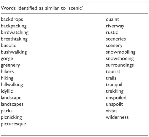
‘scenic’, for which three words are returned: ‘picturesque’, ‘scenery’ and ‘hiking’. We then search again for these three words to identify further similar words, where the model returns words such as ‘birdwatching’, ‘landscape’ and ‘unspoilt’. Table 1 lists all the words identified by this approach.

In order to identify images that the textual information suggests might be scenic, we search the title, description and tags, using a regular expression for the word ‘scenic’ (e.g. \bscenic\b) and, separately, for the word ‘scenic’ or words similar to ‘scenic’ (e.g.

\b(scenicWpicturesqueWbirdwatchingWlandscape)\b) The expression ‘\b’ allows us to search for

Estimating scenic areas

We build a base model to help us determine how scenic an area is, using the measures of population density, number of residents, and whether an area is categorised as urban, suburban or rural.

When working with spatial data, it is reasonable to assume that observations in neighbouring areas may be more or less alike simply due to their proximity, and hence may exhibit autocorrelation (Bivand et al., 2013; Harris et al., 2005). We confirm this by first carrying out a Moran’s I test, which measures whether spatial autocorrelation is present in the data. Due to the spatial autocorrelation revealed by this test (as reported in more detail below), it is not appropriate to run a simple linear regression analysis, as spatial dependencies would exist in the error term. Hence, we run our analysis using a conditional auto regressive (CAR) model as detailed below.

We then explore to what extent crowdsourced data fromFlickrandOpenStreetMap can

help improve our base model. We identify which crowdsourced variables can add power to our model using a statistical learning method as explained below.

Table 1. Identifying words similar to ‘scenic’.a Words identified as similar to ‘scenic’

backdrops quaint

backpacking riverway

birdwatching rustic

breathtaking sceneries

bucolic scenery

bushwalking snowmobiling

gorge snowshoeing

greenery surroundings

hikers tourist

hiking trails

hillwalking tranquil

idyllic trekking

landscape unspoiled

landscapes unspoilt

parks vistas

picnicking wilderness

picturesque

a

To determine which words we should consider as similar to scenic, we build aword2vecmodel (Radim and Petr, 2010, Mikolov et al., 2013). Aword2vec

model is a model which is constructed by processing a large corpus of text, in order to build a representation of the semantic meaning of each word on the basis of the contexts in which it appears. Having constructed this model, we are able to query it in order to identify words that have a similar meaning to any word of interest, such as ‘scenic’. We classify a word as being similar if the similarity between the words is more than 0.5 according to the constructed

Finally, we investigate whether models including crowdsourced variables can generate more accurate estimates of scenicness than our base model comprising measurements of population and area category alone, by comparing the Akaike weights (AICw) of each model.

CAR model

Initially proposed by Besag and colleagues (Besag, 1974; Besag et al., 1991), the CAR model captures spatial dependence between neighbours through an adjacency matrix of the areal units.

The CAR model quantifies the spatial relationship in the data by including a conditional

distribution in the error termei. The conditional distribution ofeiis thus represented as

eijejiN

X

ji

cijej

P

jicij

,

2

ei

P

jicij

!

where eji is the vector of error terms for all neighbouring areas of i; and cij denotes

dependence parameters used to represent the spatial dependence between the areas.

Using statistical learning to identity candidate variables

We use the statistical learning method of cross-validation (Hastie et al., 2009; James et al., 2013) to identify candidate variables to use in our scenic estimation models using crowdsourced data. We randomly partition the observations in our data set into a 60/40 split where 60% of the data are used as the training set and 40% of the data are used as the validation set. We ensure that each partitioned data set has an equal split of urban, suburban, and rural areas. We fit new models on the training data set including all the variables in our base model (population density, number of residents, and urban, suburban or rural categories) plus every combination of all the crowdsourced variables we have identified, as listed in Table 2. We then fit these models to estimate responses for the observations on the validation set. We then compare the resulting validation test error rates, as measured by Root Mean Square Errors (RMSE). We choose two candidate models for estimating scenicness by choosing those with the lowest RMSEs.

Akaike weights

In order to determine which model best estimates scenicness, we calculate the AICw, following the method proposed by Wagenmakers and Farrell (2004), as the AIC values themselves are challenging to interpret on their own. We derive AICws, by first identifying the model with the lowest AIC. For each model, we then calculate an AIC difference, by determining the difference between the lowest AIC and the model’s AIC. We next determine the relative likelihood of each model, following the method described in Wagenmakers and Farrell (2004). To calculate the AICws, we normalise these likelihoods, such that across all models they sum to one. The resulting AICws can be interpreted as the probability of each model given the data.

Results

A comparison of the quantity ofFlickrphotographs taken (Figure 1(a)) with a map of scenic

photos – which tend to be highly populated areas such as London and Manchester – are rated as being the least scenic. On the other hand, highly scenic areas, such as Scotland, have

a low density ofFlickrphotographs taken. This indicates that population density may be a

significant factor for estimating the scenicness of an area.

This also leads us to suppose that whether an area is urban, suburban or rural may also play a part in scenic ratings. Furthermore, Scotland, which is rated as highly scenic, is known for its beautiful rural settings. We therefore explore to what extent urban, suburban and rural areas affect scenic ratings.

We build our first model to determine how scenic an area is, drawing on these objective measurements: population density, number of residents, and urban, suburban or rural categories. As noted in the Methods section, spatial data may exhibit autocorrelation, where nearby observations may have similar values, and thereby violate the assumption

made in linear regression that observations are independent. To test whether

autocorrelation exists, we first build a linear regression model. A Moran’s I test on the residuals of the linear regression model confirms that the model exhibits significant spatial

autocorrelation in the residuals (Moran’s I¼0.127, p<0.001, N¼15,188). We therefore

build a CAR model (as described in ‘Methods’ section) that takes spatial autocorrelation into account (Bivand et al., 2013; Harris et al., 2005).

The results of the CAR model analysis reveal that low population density is associated

with areas of high scenicness (b¼ 0.285,p<0.001,N¼15,188) and the lower the number

of residents in an LSOA, the greater the scenicness (b¼ 0.0001,p<0.001,N¼15,188). We

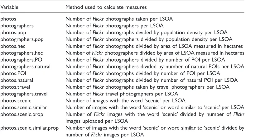
Table 2. Crowdsourced variables considered in our analysis.a

Variable Method used to calculate measures

photos Number ofFlickrphotographs taken per LSOA

photographers Number ofFlickrphotographers per LSOA

photos.pop Number ofFlickrphotographs divided by population density per LSOA photographers.pop Number ofFlickrphotographers divided by population density per LSOA photos.hec Number ofFlickrphotographs divided by area of LSOA measured in hectares photographers.hec Number ofFlickrphotographers divided by area of LSOA measured in hectares photographers.POI Number ofFlickrphotographers divided by number of POI per LSOA photographers.natural Number ofFlickrphotographers divided by number of natural POIs per LSOA photos.POI Number ofFlickrphotographs divided by number of POI per LSOA

photos.natural Number ofFlickrphotographs divided by number of natural POI per LSOA photos.travel Number ofFlickrphotographs taken by travel photographers per LSOA photographers.travel Number ofFlickrtravel photographers per LSOA

photos.scenic Number of images with the word ‘scenic’ per LSOA

photos.scenic.similar Number of images with the word ‘scenic’ or word similar to ‘scenic’ per LSOA photos.scenic.prop Number ofFlickr images with the word ‘scenic’ divided by number of Flickr

images uploaded per LSOA

photos.scenic.similar.prop Number of images with the word ‘scenic’ or word similar to ‘scenic’ divided by number ofFlickrimages per LSOA

a

PHOTOS ON

FLICKR

London Birmingham Manchester Sheffield Newcastle

Liverpool

FLICKR

PHOTOGRAPHERS

SCENIC-OR-NOT

RATING

Number of Flickr images (excluding buildings)

1 4 7 11 16 26 52 6300 1 20 400 800

Number of Flickr

photographers per LSOA

1 2.3 3.2 3.7 4 4.3 4.9 8

Average Scenic-Or-Not

rating per LSOA

Edinburgh Glasgow

Cardiff (a)

(b) (c)

Figure 1. The relationship betweenFlickrphotographs and ratings of scenicness fromScenic-Or-Notin Great Britain. (a) We create a density plot of allFlickrphotographs uploaded in 2013, geotagged as being taken in Great Britain. In order to ensure that the photographs have been taken outdoors, we exclude images that were taken in buildings. Buildings are identified using crowdsourced data fromOpenStreetMap. Inspection of the map indicates that most images are taken in areas of high population density such as London and Manchester. (b) TheScenic-Or-Notdata set comprises 217,000 images, sourced fromGeograph, covering nearly 95% of the 1 km grid squares of Great Britain. We calculate the mean scenic rating of all

Scenic-or-Notphotographs at the level of English Lower Layer Super Output Areas (LSOAs) and depict these

also find that urban and suburban areas are associated with reduced scenicness (urban

b¼ 0.260p<0.001,N¼15,188; suburbanb¼ 0.083,p<0.001,N¼15,188).

We now explore to what extent crowdsourced data from FlickrandOpenStreetMap can

add additional explanatory power to our base model. First, we investigate whether the

quantity of geotagged images uploaded to Flickr may be a proxy for visual preference of

an area. As we are interested in the perception of outdoor environments rather than indoor

environments, we also use crowdsourced data from OpenStreetMap to determine where

buildings are located, and use this data on to exclude Flickr images that have been taken

inside buildings.

We note factors that may affect the quantity ofFlickrimages besides the scenicness of an

area, and take a number of steps to correct for these issues in our analysis. First of all, we account for the fact that one photographer may take several photographs of an area. While this may reveal individual preference for an area, this may not reveal collective preference for

an area. We therefore consider only the quantity ofFlickrphotographers for each LSOA, as

we are primarily interested in the collective perception of scenicness.

Next, we consider the various reasons for people takingFlickrphotographs. For example,

people typically upload photographs to Flickr when they want to share a memory of an

event or an activity such as a birthday party (Purves et al., 2011), or they might share pictures of themselves (commonly known as ‘selfies’). People might also add valuable information related to a photograph if they are motivated to share the image with the wider public (Nov et al., 2008). We therefore attempt to mitigate the potential biases in

the uploadedFlickrphotographs, as well as identify a stronger signal of scenic images by the

following approaches: (1) we attempt to identify travel photographers and (2) we attempt to identify scenic images.

We hypothesise that Flickr photographs taken by photographers that travel are more

likely to reveal scenic preferences. We therefore count the number of LSOAs in which each

Flickr photographer has taken photos. We find the mean number of LSOAs in which

someone has taken a photograph is eight. We therefore deem a Flickr photographer a

‘travel photographer’ if they have taken photographs in more than eight LSOAs.

We also attempt to identify which images are scenic using textual data people have added to describe the image, as explained in more detail in ‘Methods’ section. We classify an image as scenic if there is a mention of ‘scenic’ or a word similar to ‘scenic’ in this textual metadata. We then count the number of images classified as scenic for each LSOA. We also include the count of images classified as scenic divided by all the images uploaded per LSOA, which gives us the proportion of images classified as scenic uploaded per LSOA.

Finally, we correct for a variety of characteristics that may affect the quantity of images uploaded in each LSOA: land area, quantity of points of interest (POI) and quantity of natural features. As LSOAs vary dramatically in size – between 1 hectare to 67,280 hectares in our analysis – and people may take more pictures in larger LSOAs, we consider to which

extent hectares affect the number of Flickr photographs taken. Certain POI, particularly

tourist attractions, such as the London Eye, Big Ben and Edinburgh Castle attract large numbers of images (Antoniou et al., 2010). This could distort the signal of whether or not the photographer considers the location scenic. We therefore consider how the quantity of POI

in each LSOA influence the number of Flickrphotographs taken.OpenStreetMap also has

data on how many natural POI exist in each LSOA. As natural POI may be associated with

scenicness, we also consider how many Flickr images are taken considering how many

We can now test whether models that include crowdsourced variables perform better than abase modelthat only includes the objective measurements (population density, number of residents, and urban, suburban or rural categories). Table 2 lists all the crowdsourced variables that we test.

Using a statistical learning approach (as specified in the Methods section), we identify two

candidate models that include crowdsourced data: (1) A simple Flickr model that, in

addition to the base model, includes the number of Flickr photographers in each LSOA

divided by the number of POI in that LSOA (variable: photographers.POI); and (2) an

extended Flickr model that, in addition to the simple Flickr model, includes the number

of images classified as scenic per LSOA (variable:photos.scenic.similar).

As in our previous analysis, we build these two candidate Flickr CAR models. In the

simple Flickr model, we find that a greater number of Flickr photographers, adjusted by

POI, is significantly associated with higher ratings of scenicness (b¼0.095, p<0.001,

N¼15,188). In the extended Flickr model, we also find that a greater number of Flickr

photographers, adjusted by POI, is significantly associated with higher ratings of

scenicness (b¼0.092, p<0.001, N¼15,188). In addition, we find that the number of

images with the word ‘scenic’ or a word similar to ‘scenic’ is significantly associated with

higher ratings of scenicness (b¼0.001,p<0.001,N¼15,188).

Finally, in order to determine whether models including crowdsourced variables can perform better than the models that only include objective measurements, we rank all

three models – the base model, the simple Flickr model, and the extendedFlickr model –

in terms of their Akaike Information Criterion (AIC) value. This provides a measure of the model fit given a set of data. In order to compare the fit of the models to each other, AIC values are transformed to AICw following the method proposed by Wagenmakers and Farrell (2004). These weights can be interpreted as the probability of each model given the data, as described in the ‘Methods’ section. This model comparison indicates that

models including crowdsourced geographic data from Flickr andOpenStreetMap provide

more accurate estimates of the scenicness of an area than models that only include objective measurements such as population density and whether an area is urban, suburban or rural (Table 3).

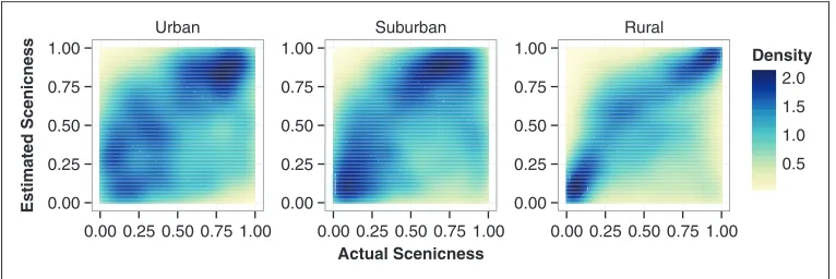
Using the most probable model, the extendedFlickrmodel, we further investigate how the

ranked estimates of the scenicness of an area compare to the ranked actual measures of the scenicness of an area in different settings (Figure 2). We find that our model is most

successful at estimating the scenicness of an area in rural settings (urban: s¼0.216,

p<0.001, N¼1,060; suburban: s¼0.225, p<0.001, N¼2,567; rural: s¼0.363, p<0.001,

N¼2,449, Kendall’s rank correlation).

Discussion

Our findings suggest that crowdsourced data from sources such as Flickr and

OpenStreetMap have the potential to reveal information about how people interact with their environment. Specifically, we find that models using crowdsourced data can generate more accurate estimates of scenicness than models comprising only traditional statistics such as population density or whether an area is urban or rural. Our results provide evidence that

measures of images uploaded to Flickr do indeed contain information that can inform

estimates of how scenic an area is.

However, while the improvement is significant, the effect size is not large. As our sample

analysis of 10,000Flickrimages indicated that around 23% of the images deemed as outdoor

Table 3. The performance of different models for estimating scenic ratings.a

Base model SimpleFlickrmodel ExtendedFlickrmodel

Log of population density 0.285*** 0.274*** 0.270***

All residents 0.000*** 0.000*** 0.000***

Suburban 0.083*** 0.087*** 0.088***

Urban 0.260*** 0.26*** 0.263***

photographers.POI 0.095*** 0.092***

photos.scenic.similar 0.001***

No of observations 15,188 15,188 15,188

AIC 43,045 42,850 42,830

AICd 215 20 0

AICw <0.001 <0.001 >0.999

a_{Regression coefficients for CAR models estimating scenic ratings based on the validation data set (*p<0.05, **p<0.01,}

***p<0.001). The set of observations are randomly partitioned into a 60/40 split, where 60% of the data are used as the training set and 40% as the validation set. Each partitioned data set has an equal split of urban, suburban and rural areas. The analysis is carried out at the level of Lower Layer Super Output Areas (LSOAs). The simpleFlickrmodel includes an additional variable: the number of images taken by unique photographers divided by the number of points of interest (photographers.POI). The extendedFlickrmodel includes a further additional variable: the number of images with the word ‘scenic’ or word similar to ‘scenic’ per LSOA (photos.scenic.similar). Here, we present the results of evaluating the models on the entire data set. In order to determine which model offers the best estimation power, we rank all three in terms of their AIC values. In order to compare the fit of the models to each other, AIC values are transformed to Akaike weights (AICw) following the method proposed by Wagenmakers and Farrell (2004). We find that the extendedFlickr

model with the additional crowdsourced geographic variables has the greatest estimation power. These results provide evidence that models including crowdsourced data have greater power to estimate the scenicness of an area.

Estimated Scenicness

Urban

Actual Scenicness

Suburban Rural

0.00 0.25 0.50 0.75 1.00

0.00 0.25 0.50 0.75 1.00 0.00 0.25 0.50 0.75 1.00

0.00 0.25 0.50 0.75 1.00 0.00 0.25 0.50 0.75 1.00

0.00 0.25 0.50 0.75 1.00 0.5 1.0 1.5 2.0

Density

We found no evidence in support of our hypothesis that travel photographers would give us a useful metric of the scenicness of an area. Visual analysis of the photographs uploaded

by the most prolific Flickr travel photographers reveals that many of them useFlickr for

curated content such as bus and train spotting (an observation also reported by Gliozzo

et al., 2016). If the primary motivation of many of the photographers onFlickr is only to

post content on a particular subject, then this would distort the estimate thatFlickrdata may

provide of the scenicness of an area.

We aim to mitigate this effect by only including images that we identify as being related to scenicness through our analysis of textual data associated with each image. While this approach improves our results, the overall impact from this approach still is not strong enough to dramatically improve our scenicness estimates.

Finally, we consider why the performance of our analysis is worse in urban and suburban

areas. Our analysis focuses on images with locations that OpenStreetMap data indicated

have been taken outside buildings. However, we find that a neural network trained to extract

information from images of outdoor and indoor environments, Places CNN(Zhou et al.,

2014), produces different classifications for some of these images. Specifically, when

analysing a sample of 10,000 images classified as outdoor using OpenStreetMap data, we

find that Places CNN classifies 35% of the images taken in urban areas and 24% of the

images taken in suburban areas as indoor images. In rural areas, only 14% of the images

classified as outdoor images usingOpenStreetMapdata are classified as indoor images with

Places CNN. We suggest that higher building density in urban and suburban areas may mean that higher location accuracy is required to avoid misclassification between indoor and outdoor locations, such that a greater proportion of misclassifications is to be expected. This problem is likely to be exacerbated due to reduced functionality of GPS location technology

in built-up areas.OpenStreetMapdata can also suffer from lack of positional accuracy and

lack of completeness (Haklay, 2010; Zielstra and Hochmair, 2013). Urban and suburban

areas may be more likely to have buildings that have yet to be added to theOpenStreetMap

buildings data. Our OpenStreetMap data on POI may also contain a great deal of

uncertainty, particularly in urban and suburban areas where there are likely to be a greater number of POI and thus a higher chance of inaccuracies. Furthermore, we note that Scenic-Or-Not ratings are provided on a 1 km grid square basis. At the same time urban and suburban LSOAs are likely to be smaller than rural LSOAs: rural LSOAs range from 2 to 67,280 hectares; suburban LSOAs range from 4 to 5,362 hectares; and urban LSOAs range from 1 to 4,804 hectares. Information on the scenicness of urban and suburban areas may therefore be lower in quality, due to a lower number of scenicness ratings per LSOA.

Conclusion

We investigate whether the vast quantity of data uploaded to the Internet could help us identify which areas of Great Britain people consider to be scenic. We analyse data from

geotagged images uploaded to Flickr, combined with crowdsourced geographic data from

OpenStreetMap, in order to see if such data can provide improvements of scenic estimations.

We validate our findings using the website Scenic-Or-Not, which crowdsources ratings of

Flickr photographers, taking into account the number of POI (as obtained through

OpenStreetMap data) in each LSOA and (2) the number of images with the word ‘scenic’ or a word similar to ‘scenic’ per LSOA.

We also find that models drawing on data fromFlickrandOpenStreetMapproduce more

accurate estimates of scenicness in rural neighbourhoods than in urban and suburban areas. This may be due to the plurality of reasons for which people upload photographs in urban and suburban neighbourhoods: for instance, creating a memory of an event such as a birthday party or a sporting event. Urban and suburban LSOAs are also likely to contain a greater number of unidentified indoor images in our analysis as such areas are more likely

to contain buildings that may either be missing from theOpenStreetMapdata or for which

theOpenStreetMapdata is positionally inaccurate. Similarly, functionality of GPS location technology used to locate photographs is likely to be reduced in urban and suburban areas. Finally, our urban and suburban scenic ratings may be less accurate than those in rural

areas, due to the presence of smaller LSOAs which contain fewer Scenic-Or-Notimages in

urban and suburban areas. Further research will need to be conducted in order to mitigate these factors.

Nonetheless, analysis of crowdsourced data does seem to provide valuable information on how people perceive their everyday environments. Our results suggest that by exploiting data gathered from our everyday interactions with the Internet, scientists and policy-makers alike may be able to develop a better understanding of people’s subjective experience of the environment in which they live.

Authors note

This publication is supported by multiple data sets, which are openly available at locations described in the ‘Data and methodology’ section and cited in the reference section.

Declaration of conflicting interests

The author(s) declared no potential conflicts of interest with respect to the research, authorship, and/or publication of this article.

Funding

The author(s) disclosed receipt of the following financial support for the research, authorship, and/or publication of this article: HSM and TP acknowledge the support of the Research Councils UK via grant EP/K039830/1. CIS is grateful for support provided by a Warwick Business School Doctoral Scholarship. CIS, HSM and TP were also supported by the Alan Turing Institute under the EPSRC grant EP/N510129/1. This research utilized Queen Mary’s MidPlus computational facilities, supported by QMUL Research-IT and funded by EPSRC grant EP/K000128/1.

References

Antoniou V, Morley J and Haklay M (2010) Web 2.0 geotagged photos: Assessing the spatial

dimension of the phenomenon.Geomatica64(1): 99–110.

Batty M (2013) Big data, smart cities and city planning.Dialogues in Human Geography3: 274–279.

Besag J (1974) Spatial interaction and the statistical analysis of lattice systems.Journal of the Royal

Statistical Society, Series B36(2): 192–236.

Besag J, York J and Mollie´ A (1991) Bayesian image restoration, with two applications in spatial

Bishop ID and Hulse DW (1994) Special issue landscape planning: Expanding the Tool KitPrediction

of scenic beauty using mapped data and geographic information systems.Landscape and Urban

Planning30(1): 59–70.

Bivand RS, Pebesma E and Go´mez-Rubio V (2013)Applied Spatial Data Analysis with R. New York,

NY: Springer.

Botta F, Moat HS and Preis T (2015) Quantifying crowd size with mobile phone and Twitter data.

Royal Society Open Science2(5): 150162.

Casalegno S, Inger R, DeSilvey C, et al. (2013) Spatial Covariance between aesthetic value & other

ecosystem services.PLoS One8(6): e68437.

de Vries S, Verheij RA, Groenewegen PP, et al. (2003) Natural environments – Healthy environments?

An exploratory analysis of the relationship between greenspace and health. Environment and

Planning A35(10): 1717–1731.

Dunkel A (2015) Visualizing the perceived environment using crowdsourced photo geodata.Landscape

and Urban Planning, Special Issue: Critical Approaches to Landscape Visualization142: 173–186. Dykes J, Purves R, Edwardes A, et al. (2008) Exploring volunteered geographic information to

describe place: visualization of the ‘Geograph British Isles’ collection. In:Proceedings of the GIS

research UK 16th annual conference. Manchester: Manchester Metropolitan University, pp. 256–267.

GeoFabrik (2016) OpenStreetMap data on buildings, points of interests and natural points of interest. Available at: http://www.geofabrik.de (accessed 20 July 2016).

Giles-Corti B, Broomhall MH, Knuiman M, et al. (2005) Increasing walking: How important is

distance to, attractiveness, and size of public open space? American Journal of Preventive

Medicine28(2 suppl 2): 169–176.

Girardin F, Calabrese F, Dal Fiore F, et al. (2008) Digital footprinting: Uncovering tourists with

user-generated content.IEEE Pervasive computing7(4): 36–43.

Gliozzo G, Pettorelli N and Haklay MM (2016) Using crowdsourced imagery to detect cultural

ecosystem services: A case study in South Wales, UK.Ecology and Society21(3): 6.

Goodchild MF (2007) Citizens as sensors: The world of volunteered geography.GeoJournal 69(4):

211–221.

Graham M and Shelton T (2013) Geography and the future of big data, big data and the future of

geography.Dialogues in Human Geography3: 255–261.

Greˆt-Regamey A, Bishop ID and Bebi P (2007) Predicting the scenic beauty value of mapped landscape

changes in a mountainous region through the use of GIS.Environment and Planning B: Planning and

Design34(1): 50–67.

Haklay M (2010) How good is volunteered geographical information? A comparative study of

OpenStreetMap and ordnance survey datasets.Environment and Planning B: Planning and Design

37(4): 682–703.

Haklay M, Singleton A and Parker C (2008) Web Mapping 2.0: The neogeography of the GeoWeb.

Geography Compass2(6): 2011–2039.

Harris R, Sleight P and Webber R (2005) Geodemographics, GIS, and Neighbourhood Targeting.

Chichester: Wiley.

Hastie TJ, Tibshirani RJ and Friedman JH (2009)The Elements of Statistical Learning: Data Mining,

Inference, and Prediction. New York, NY: Springer.

James G, Witten D, Hastie T, et al. (2013)An Introduction to Statistical Learning. New York, NY:

Springer.

Kaczynski AT, Potwarka LR and Saelens BE (2008) Association of park size, distance, and features

with physical activity in neighborhood parks.American Journal of Public Health98(8): 1451–1456.

Kardan O, Gozdyra P, Misic B, et al. (2015) Neighborhood greenspace and health in a large urban

center.Scientific Reports5: 11610.

King G (2011) Ensuring the data-rich future of the social sciences.Science331(6018): 719–721.

Lazer D, Pentland A, Adamic L, et al. (2009) Computational social science. Science 323(5915):

Maas J, Verheij RA, Groenewegen PP, et al. (2006) Green space, urbanity, and health: how strong is

the relation?Journal of Epidemiology & Community Health60(7): 587–592.

Maas J, Spreeuwenberg P, van Winsum-Westra M, et al. (2009) Is green space in the living

environment associated with people’s feelings of social safety.Environment and Planning A41(7):

1763–1777.

MacKerron G and Mourato S (2013) Happiness is greater in natural environments. Global

Environmental Change23(5): 992–1000.

Mikolov T, Sutskever I and Chen K, et al. (2013) Distributed representations of words and phrases and

their compositionality. In:Advances in neural information processing systems, pp.3111–3119.

Mitchell R and Popham F (2007) Greenspace, urbanity and health: Relationships in England.Journal

of Epidemiology & Community Health61(8): 681–683.

Mitchell R and Popham F (2008) Effect of exposure to natural environment on health inequalities: An

observational population study.Lancet372(9650): 1655–1660.

Moat HS, Preis T, Olivola CY, et al. (2014) Using big data to predict collective behavior in the real

world.Behavioral and Brain Sciences37(1): 92–93.

National Records of Scotland (2012) Scotland’s Census 2011. Available at: http://www. scotlandscensus.gov.uk/ (accessed 16 July 2014).

Neis P and Zipf A (2012) Analyzing the contributor activity of a volunteered geographic information

project – The case of OpenStreetMap. ISPRS International Journal of Geo-Information 1(2):

146–165.

Nov O, Naaman M and Ye C (2008) What drives content tagging: The case of photos on Flickr. In:

Proceedings of the 2008 conference on human factors in computing systems, Florence, Italy, 5–10 April 2008, pp. 1097–1100. New York, NY: ACM.

O’Brien O, Cheshire J and Batty M (2014) Mining bicycle sharing data for generating insights into

sustainable transport systems.Journal of Transport Geography34: 262–273.

Office for National Statistics (2012) 2011 Census Data for England and Wales. Available at: https:// www.nomisweb.co.uk/census/2011 (accessed 16 July 2014).

Office for National Statistics (2013) The 2011 Rural–urban classification for small area geographies. Available at: http://geoportal.statistics.gov.uk/ (accessed 16 July 2014).

Palmer JF (2004) Using spatial metrics to predict scenic perception in a changing landscape: Dennis,

Massachusetts.Landscape and Urban Planning69(2–3): 201–218.

Preis T, Moat HS, Bishop SR, et al. (2013) Quantifying the digital traces of hurricane sandy on Flickr.

Scientific Reports3: 3141.

Purves R, Edwardes A and Wood J (2011) Describing place through user generated content.First

Monday16(9).

Radim Rˇ and Petr S (2010) Software Framework for Topic Modelling with Large Corpora

Proceedings of the LREC 2010 Workshop on New Challenges for NLP Frameworks. Valletta, Malta: ELRA, 45–50.

Schirpke U, Tasser E and Tappeiner U (2013) Predicting scenic beauty of mountain regions.Landscape

and Urban Planning111: 1–12.

Scottish Government (2012) 2011–2012 Urban–Rural Classification. Available at: http://www.gov. scot/Topics/Statistics/About/Methodology/UrbanRuralClassification/

UrbanRuralClassification201112 (accessed 16 July 2014).

Seresinhe CI, Preis T and Moat HS (2015) Quantifying the impact of scenic environments on health.

Scientific Reports5: 16899.

Seresinhe CI, Preis T and Moat HS (2016) Quantifying the link between art and property prices in

urban neighbourhoods.Royal Society Open Science3: 160146.

Stadler B, Purves R and Tomko M (2011) Exploring the relationship between Land Cover and

subjective evaluation of scenic beauty through user generated content. In:Proceedings of the 25th

international cartographic conference, Paris, France, July 2011.

Sui D, Elwood S and Goodchild M (2013) Crowdsourcing Geographic Knowledge: Volunteered

Sugiyama T, Francis J, Middleton NJ, et al. (2010) Associations between recreational walking and

attractiveness, size, and proximity of neighborhood open spaces.American Journal of Public Health

100(9): 1752–1757.

Tenerelli P, Demsˇar U and Luque S (2016) Crowdsourcing indicators for cultural ecosystem services: A

geographically weighted approach for mountain landscapes.Ecological Indicators64: 237–248.

van den Berg AE, Maas J, Verheij RA, et al. (2010) Green space as a buffer between stressful life events

and health.Social Science & Medicine70(8): 1203–1210.

Vespignani A (2009) Predicting the behavior of techno-social systems.Science325(5939): 425–428.

Wagenmakers E-J and Farrell S (2004) AIC model selection using Akaike weights. Psychonomic

Bulletin & Review11(1): 192–196.

White MP, Alcock I, Wheeler BW, et al. (2013) Would you be happier living in a greener urban area? A

fixed-effects analysis of panel data.Psychological Science24(6): 920–928.

Wood SA, Guerry AD, Silver JM, et al. (2013) Using social media to quantify nature-based tourism

and recreation.Scientific Reports3: 2976.

Zaltz Austwick M, O’Brien O, Strano E, et al. (2013) The structure of spatial networks and

communities in bicycle sharing systems.PLoS One8(9): e74685.

Zhou B, Lapedriza A, Xiao J, et al. (2014) Learning deep features for scene recognition using places

database. In: Advances in neural information processing systems 27, Montreal, Canada, 8–13

December 2014. La Jolla, CA: Neural Information Processing Systems, pp. 487–495.

Zielstra D and Hochmair HH (2013) Positional accuracy analysis of Flickr and Panoramio images for

selected world regions.Journal of Spatial Science58(2): 251–273.

Chanuki Illushka Seresinhe is a doctoral researcher at the Data Science Lab, Warwick Business School, currently spending a PhD enrichment year at the Alan Turing Institute. Having previously worked in the design sector for over 10 years, Chanuki is now exploring how online data from such sources as Flickr and Twitter can help us understand how the aesthetics of the environment impacts human wellbeing. The results of her research have

been featured by press worldwide, by outlets such as The Guardian, The Telegraph, ITV

NewsandScientific American.

Dr Helen Susannah Moat is an Associate Professor of Behavioural Science at Warwick Business School, where she co-directs the Data Science Lab. She is also a Faculty Fellow at the Alan Turing Institute. Moat’s research investigates whether online data from sources such as Google, Wikipedia and Flickr can help us measure and predict human behaviour and wellbeing. The results of her research have been featured by television, radio and press

worldwide, by outlets such as CNN, BBC,The Guardian, andNew Scientist. Moat has also

acted as an advisor to government and public bodies on the predictive capabilities of big data.

Dr Tobias Preis is an Associate Professor of Behavioural Science and Finance at the University of Warwick where he co-directs the Data Science Lab. Preis is also a Faculty Fellow at the Alan Turing Institute. His recent research has aimed to analyse and predict real world behaviour with the volumes of data being generated by our interactions with technology, using data from Google, Wikipedia, Flickr and other sources. His research is

frequently featured in the news, by outlets including the BBC, the New York Times, the