Two extensions of Kingman's GI/G/1 bound

warwick.ac.uk/lib-publications

Manuscript version: Author’s Accepted Manuscript

The version presented in WRAP is the author’s accepted manuscript and may differ from the

published version or Version of Record.

Persistent WRAP URL:

http://wrap.warwick.ac.uk/111282

How to cite:

Please refer to published version for the most recent bibliographic citation information.

If a published version is known of, the repository item page linked to above, will contain

details on accessing it.

Copyright and reuse:

The Warwick Research Archive Portal (WRAP) makes this work by researchers of the

University of Warwick available open access under the following conditions.

Copyright © and all moral rights to the version of the paper presented here belong to the

individual author(s) and/or other copyright owners. To the extent reasonable and

practicable the material made available in WRAP has been checked for eligibility before

being made available.

Copies of full items can be used for personal research or study, educational, or not-for-profit

purposes without prior permission or charge. Provided that the authors, title and full

bibliographic details are credited, a hyperlink and/or URL is given for the original metadata

page and the content is not changed in any way.

Publisher’s statement:

Please refer to the repository item page, publisher’s statement section, for further

information.

Florin Ciucu

University of Warwick

Felix Poloczek

ABSTRACT

A simple bound in GI/G/1 queues was obtained by Kingman using

a discrete martingale transform [30]. We extend this technique to

1) multiclassΣGI/G/1 queues and 2) Markov Additive Processes

(MAPs) whose background processes can be time-inhomogeneous

or have an uncountable state-space. Both extensions are facilitated

by a necessary and sufficient ordinary differential equation (ODE)

condition for MAPs to admit continuous martingale transforms.

Simulations show that the bounds on waiting time distributions

are almost exact in heavy-traffic, including the cases of 1)

hetero-geneous input, e.g., mixing Weibull and Erlang-k classes and 2)

Generalized Markovian Arrival Processes, a new class extending

the Batch Markovian Arrival Processes to continuous batch sizes.

KEYWORDS

Queueing; Markov and Non-Renewal Processes; Stochastic Bounds

ACM Reference Format:

Florin Ciucu and Felix Poloczek. 2018. Two Extensions of Kingman’s GI/G/1 Bound. InProceedings of ACM conference.ACM, New York, NY, USA, Arti-cle 4, 18 pages.

1

INTRODUCTION

A milestone in queueing theory was relaxing the often implicit

assumption that interarrival times in GI/G/1 queues are statistically

independent. One such extension, applicable in manufacturing and

production systems, is the multiclassΣGI/G/1 queue in which mul-tiple classes of jobs, each with its own arrival (renewal) process, are

merged. Due to the general lack of closure of renewal processes,

let alone the general lack of stationarity of the merged process,

the analysis of theΣGI/G/1 queue is challenging. Several studies

in heavy-traffic regimes addressed functional central limits (e.g.,

of the waiting times) [27], approximations (e.g., of the workload)

with a one-dimensional reflecting Brownian motion [17], or Laplace

transforms (e.g., of the waiting times) [6].

Another extension also emerging in the 1970s was driven by the

non-renewal traffic characteristics in packet switches [2, 32]. Two

widely studied models accounting for ‘bursty’ traffic are Markov

Modulated Fluid (MMF) and Markov Modulated Poisson Process

(MMPP). The former was proposed in the seminal paper [2] by

rep-resenting traffic as (continuous) ‘fluid’ evolving at some constant

rate, depending on a modulating Markov process; queues with MMF

input can be exactly analyzed using ODEs and matrix analysis;

re-lated methods include spectral decomposition [1] or Wiener-Hopf

Permission to make digital or hard copies of part or all of this work for personal or

classroom use is granted without fee provided that copies are not made or distributed

for profit or commercial advantage and that copies bear this notice and the full citation

on the first page. Copyrights for third-party components of this work must be honored.

For all other uses, contact the owner /author(s). ACM conference, 2018

© 2018 Copyright held by the owner/author(s).

ACM ISBN 123-4567-24-567/08/06.

factorization [45]. MMPP is a more accurate ‘packetized’ version of

MMF, i.e., traffic evolves as a Poisson process with state dependent

rates according to a modulating Markov process; the typical

queue-ing analysis rests on matrix analytical techniques [25] or spectral

decompositions [1, 20]. A common challenge of analyzing MMF and

MMPP is the underlying numerical complexity, which can become

prohibitive when a large number of sources are multiplexed [48].

For related discussions and more comprehensive reference lists

see [33] and [23].

A popular method to analyze queues with MMF and MMPP input

is effective bandwidth [19]. Advantages include the availability

of exact (asymptotic) results, negligible computational cost when

multiplexing many sources, and simplicity in the sense that many

arrival processes can be analyzed in a unified manner. However, this

method can yield inaccurate (non-asymptotic) results unless the

input is Poisson [13, 48]. A related technique with similar features

is the probabilistic network calculus [34].

In this paper we develop a unified analysis of queues with two

broad classes of non-renewal arrivals: 1) the multiclassΣGI/G/1 queue and 2) queues with Markov Additive Processes (MAPs). Our

framework provides (non-asymptotic) stochastic bounds (e.g., on

waiting time distributions) by extending an approach of

King-man [30] who obtained such bounds in GI/G/1 queues by first

constructing martingale transforms and then using martingale

prop-erties. While this approach has often been used [4, 18, 40, 41, 46],

our novelty is a link between MAP martingales and a necessary and

sufficient ODE condition. This applies to general MAPs, whereby

the background process can be inhomogeneous or have an

un-countable state-space; moreover, the martingales are constructed in

continuous-time. These three features altogether are instrumental to the analysis of theΣGI/G/1 model.

Besides generality, the proposed method can be applied in a

rather straightforward manner. The ODE condition is elementary,

and in particular it immediately lends itself to a MMF martingale

which was obtained in [21] using an involved argument. We

inves-tigate several other scenarios, e.g.,ΣWeibull/G/1,ΣErlang-k/G/1,

ΣWeibull+ΣErlang-k/G/1 (a mix of Weibull and Erlang-k classes), and queues with MMF, MMPP, Markovian Arrival Processes (MArPs),1

and Generalized Markovian Arrival Processes (GMArP)2.

Remark-ably, the method retains the key advantage of effective bandwidth,

i.e., a straightforward analysis with negligible numerical

complex-ity in multiplexing scenarios. Additionally, the bounds are shown

through simulations to be almost exact in heavy-traffic. The method

can be easily extended to account for non-stationary services and

scheduling.

The highlights of this paper are:

1

We adopt the acronyms MAP and MArP for Markov Additive and Arrival, respectively,

Processes; see [4], p. 302.

2_{GMArP is our own generalization of Batch Markovian Arrival Processes (BMArPs),}

•A key result enablingcontinuousmartingale constructions from general MAPs by solving ODEs (Lemmas 5 and 6).

•Providing (almost) explicit and closed-form bounds on wait-ing time distributions in multiclassΣGI/G/1 queues, includ-ing heterogeneous scenarios (Examples 1-3 in § 4).

•Several simulations illustrating almost exact bounds in heavy-traffic.

•Linear time computational complexity in analyzing queues with a superposition of GMArPs (§ 5.3). Effective bandwidth

achieves the same complexity but with very poor numerical

accuracy, whereas exact results are typically subject to an

exponential complexity.

•The overall method extends to random and possibly non-stationary service, using roughly the same underlying

re-sults.

An important auxiliary result for future studies is

•Isolatinga singlesource for numerical inaccuracies in King-man’s technique (Lemma 2).

In the rest of the paper we first summarize Kingman’s technique

and give new insight into the bounds’ (in)accuracy. In § 3 we

pro-vide the main technical result of the paper. Several applications to

multiclassΣGI/G/1 and Markov Additive Processes (MAPs) queues are considered in § 4 and § 5. In § 6 we provide a more

compre-hensive discussion on related work, and also comment on possible

extensions of the proposed technique. We conclude the paper in § 7.

Appendices § A and § B provide detailed proofs and additional

nu-merical results.

2

KINGMAN’S BOUND IN SPACE AND TIME

DOMAIN QUEUEING MODELS

In this section we summarize Kingman’s [30] martingale-based

technique in two queueing models:

•Queueing models in the space domain, i.e., GI/G/1 queues (the model originally solved in [30]) and discuss their

ex-tension to multiclassΣGI/G/1 queues (whose input is not GI due to the lack of closure of renewal processes under

multiplexing, unless Poisson);

•Queueing models in the time domain, i.e., queues with gen-eral Markov Additive Processes (MAPs) comprising many

arrival models subject to correlation such as Markov Fluids

(MFs), Markov Modulated Poisson Processes (MMPPs), or

Markovian Arrival Processes (MArPs).

The purpose of this summary is to illustrate the key ideas and

similarities in the two models, relative to Kingman’s technique, and

to thus justify the development of a “unified" analysis.

2.1

Space Domain

The classical queueing model consists of two sequences of

iden-tically distributed interarrival times(T_i)_i∈

N(when do jobs arrive

at some queueing server/station?) and service times(S_i)_i∈

N(how

long does each job take to being served?). A typical assumption is

that(T_i)_i and(S_i)_iare mutually independent. This is theGI/G/1

queue.

2.1.1 Kingman’s Bound.While an exact and computationally tractable analysis of queues with general distributions is hard, an

approximate solution (in terms of stochastic bounds) can be quickly

given. Focusing on the waiting timeW_n(how long does thenthjob

wait in the queue prior to being served?), its distribution converges

to that of

W :=sup

n≥0

{U1+U2+· · ·+Un}, (1)

whereU_n:=S_n−T_nforn≥1 and subject to the stability condition

E[Un]<0 (by convention, whenn=0, the corresponding element in the ‘sup’ is 0) (see, e.g., Proposition 2.1 in [44]).

The key idea to approximateW’s distribution is a duality

be-tween stationary distributions and first passage probabilities for

random walks, i.e.,

P(W ≥σ)=P(T <∞) , (2)

whereT := inf{n:U1+· · ·+Un ≥σ}is the first passage time

(also a stopping time)3. Let the exponential martingale

Xn:=eθ(U1+U2+···+Un),

whereθ>0 satisfies_E h

eθUni₌1 (its existence is guaranteed by

stability). Then, according to the optional sampling theorem for

some finiten

1=_E[X0]=E[XT∧n]=E[XT∧n1T≤n]+E[XT∧n1T>n]

≥_E[X_T∧n1_T≤n]=_E[X_T1_T≤n]

=Eheθ(U1+U2+···+UT) 1_T≤n

i

≥eθ σE[1_T≤n]=eθ σ_P(T ≤n) .

(3)

The need for the parametern stems from a technicality of the

optional sampling theorem. By takingn→ ∞the final result is

Theorem 1. (Kingman’s Bound)In the model above

P(W ≥σ) ≤e−θ σ . (4)

The result is quite general in terms of the distributions ofT_iand Si; service times must however have a moment generating function, otherwise,θcould not be constructed as above. Note also that the

result is (almost) explicit, except for the construction ofθwhich

generally requires a numerical procedure.

2.1.2 On the Bound’s Accuracy.There are two inequalities in the derivations of Kingman’s bound from (3). We next show that

the first one holds in the limit as an equality:

Lemma 2. In the model above

lim

n→∞E[XT∧n1T>n]=0.

Proof. Construct the stopped martingale

Yn:=X_T∧n

which satisfiesXn1_T>n =Yn1_T>n. We show next thatYnis uni-formly integrable.

Fixingε>0 andn≥0 we need to findK<∞, independent of n, such that

E Yn1_Y

n>K

<ε.

3

The same idea was also used in risk analysis, whereby the right-hand side in (2) has

Let us rewrite

E Yn1_Y

n>K

=E

XT∧n1_T>n1_Y

n>K

+E

XT∧n1_T≤n1_Y

n>K

=E

Xn1_T>n1_X

n>K

+E

XT1_T≤n1_X

T>K

. (5)

From the definition ofT, the first term in the sum is 0 whenK> eθ σ. Rewrite the second term asEX_T1_T≤n1_X

T1_T≤n>K

. From

the second line of (3), withn → ∞, we obtain thatX_T1_T<∞is

integrable, and therefore (see, e.g., [50], p. 127) there exists aK<∞ such that

E

XT1_T<∞1_X

T1_T<∞>K

<ε. SinceX_T1_T≤n1_X

T1_T≤n>K ≤XT1T<∞1_X

T1_T<∞>K it then follows

that the second term in (5) can be made arbitrarily small. Hence, Ynis uniformly integrable.

According to the martingale convergence theorem (see, e.g., [50],

p. 134),Y :=limnYnexistsa.s.(and also inL1). We finally obtain that

lim

n→∞E[XT∧n1T>n]=n→∞lim E[Xn1T>n]=E

h lim

n Xn1T>n

i

=E

h lim

n Yn1T>n

i

=E

h lim

n Ynlimn 1T>n

i

=E

h lim

n Yn1T=∞

i

=E

h lim

n Xn1T=∞

i

≤_Ehlim

n Xn

i

=0.

In the first line we could exchange the limit with the expectation

from the bounded convergence theorem (the definition ofTimplies

thatX_T∧n1_T>n ≤eθ σ). In the second line we could split the limit of a product in the product of limits due to thea.s.convergence

ofY_n. In the last line we used the fact thatU₁+U₂+· · ·+U_nis a

divergent random walk with negative drift.

The previous result indicates that the accuracy of Kingman’s

bound reduces to that of the straightforward bound

E h

eθ(U1+U2+···+UT) 1_T≤n

i

≥eθ σ_P(T ≤n)

from the last inequality in (3). A refinement was provided by Ross [46],

i.e.,

sup

y≥0

K(y)eθ σ_P(T ≤n) ≥_Eheθ(U1+U2+···+UT)₁ T≤n

i

≥inf

y≥0K

(y)eθ σ_P(T ≤n) , (6)

where

K(y)=E h

eθ(U1−y)_|U

1≥y

i .

These bounds immediately lend themselves to bounds on the

wait-ing time distribution:

Lemma 3. (Ross’ Bounds)In the model above

1

sup_y≥0K(y)e

−θ σ _≤

P(W ≥σ) ≤ 1

infy≥0K(y)

e−θ σ _. (7)

Remarkably, these bounds areexactfor the GI/M/1 queue (see [46]).

As a side remark, the proof for the lower bound in (6) uses an

in-genious argument involving an additional stopping time. Using

Lemma 2, however, the lower bound can be derived exactly as the

upper bound, except for replacing the ‘inf ’ with ‘sup’.

We give an alternative proof of Lemma 3 in Appendix § A which

can be immediately extended to generalize Ross bound from (6) to

the case when(U_n)_nis a homogeneous Markov chain.

2.1.3 Open Question:ΣGI/G/1.Consider the multiclassΣGI/G/1 queue, whereby the arrivals are driven by multiple renewal

se-quences(Tk

i )i withk=1,2, . . . Unless the individual sequences are exponentially distributed, the aggregate interarrival process

(essentially the spacings of order statistics) is not a renewal

pro-cess. Consequently, the corresponding processX_nis no longer a

martingale and the above method fails. An additional complication

is that, in general, the aggregate interarrival process is not even

stationary, and hence the existence of a steady-state forWnis not guaranteed by Loynes’ condition for G/G/1 queues (which requires

the stationarity of the sequence(Ti,Si)i andE[Si]<E[Ti]). Obtaining queueing bounds in multiclassΣGI/G/1 queues, alike (4), is open. The related literature include exact results in terms of

Laplace transforms (see Theorem 4 in [6]) and approximations on

the expected waiting timeW in heavy-traffic (see Proposition 1

in [6]). Our contribution is the derivation of closed-form stochastic

bounds on thedistributionof W, alike in the GI/G/1 case.

2.2

Time Domain

The other common queueing model consists of a compound arrival

processA(t)(how many jobs arrived by timet?) and a server pro-cessing the arrivals at some rate (either constant or random). The

indextrepresents ‘time’, whereas the indexnin the previous model

represents ‘space’ (i.e., job number).

Assume a continuous-time model, a constant rateC>0 for the

server, and a stability condition lim sup_t A_t(t) <C. Focusing on the backlog processQ(t)(how many jobs are in the queue at time t), under certain stationarity and ergodicity conditions, a limiting distribution ofQ(t)exists, and that is equal to that of

Q:=sup

t≥0

{A(t) −Ct} . (8)

(we assume thatA(t)is a reversible process to simplify notation).

To compute stochastic bounds on the distribution ofQ,

King-man’s technique can be extended from the space to the time domain.

One has to first construct an appropriate martingale, e.g.,

Xt :=eθ(A(t)−Ct),

in the case whenA(t)has independent increments, under an appro-priate condition onθ. Following the same steps as before, the same

elegant approximation can be obtained

P(Q≥σ) ≤e−θ σ .

(For a complete proof in the general case with not necessarily

independent increments see Theorem 7.)

An important observation about the technique is that it does

not require the existence of a steady-state (non-ergodic Markovian

arrival processes can be addressed). The explanation is that the

produced backlog bounds are transient, i.e., they hold for_P(Q(t) ≥ σ)for any timet; the same observation holds in the space domain. An advantage of the time domain model is its suitability to

en-code the correlation structure in the arrivals (e.g., driven by some

Markov process). Moreover, analyzing queues with multiplexed

Based on this last observation, we will analyze the multiclass

ΣGI/G/1 queue by framing the model in the time domain where multiplexing is seemingly ‘easy’ (see § 4). What is noteworthy is that

the martingale construction in the transformed domain is driven

by the same general/unified result which provides conditions for

the martingale construction from pure time-domain based arrivals.

3

A MARTINGALE TRANSFORM VIA ODE

Here we present the main result of this paper, i.e., a necessary and

sufficient condition forMarkov Additive Processes(MAPs) to admit

martingale representations. In a continuous-time model, we adopt

a simplified definition of a MAP by Pacheco and Prabhu [39] (for a

more general version see [14]):

Definition 4. A bivariate process(A(t),Mt)tis aMarkov Addi-tive Processif and only if

(1) the pair(A(t),Mt)is a Markov process in_R2, (2) A(0)=0andA(t)is nondecreasing,

(3) the (joint and conditional) distribution of

(A(s,t),Mt |A(s),Ms)

depends only onMs.

Mt is abackground processandA(t)is an additive processes counting arrivals up to timet; we writeA(s,t):=A(t) −A(s). Note thatM_tis a Markov process andA(t)has conditionally independent

increments (conditioning on the states ofMt).

Next we give the main result, first in the (time) homogenous

case, i.e., the law_P(A(s+τ,t+τ) ≤x,Mt+τ =y|Ms+τ =z)is in-variant under the time shiftτ. First, denote by ‘Im’ theimageof a

function, e.g., Im(M_t)is the set of states ofM_t.

Lemma 5. (Time-Homogeneous Case)Consider a time-homogenous

Markov Additive Process(A(t),Mt), a random functionh: Im(M) → R+, the parametersy∈Im(M),C,θ >0, and define fors≥0

φy(s):=_E h

h(Ms)eθ(A(s)−Cs)

M0=y

i .

Then _dsdφy(s)

_s=

0=

0for ally∈Im(M)if and only if the process

h(Mt)eθ(A(t)−Ct) (9) is a martingale relative to the natural filtration.

An explicit exponential martingale for MAPs is given in

As-mussen [4] (see Proposition 2.4, p. 312) by solving for an

eigen-value/vector problem. In connection to this result, Lemma 5 is

more general in that the state-space ofM_t can be uncountable

(e.g.,_R); moreover, the lemma can be immediately extended to the

time-inhomogeneous case (see Lemma 6). These two features are

instrumental for the later applications. An additional advantage

of Lemma 5 is that the necessity of the differentiability condition

ensures the uniqueness of exponential martingales of the form from

Eq. (9) for several MAP examples treated in § 5.

We remark that the sufficiency of the differentiability

condi-tion is trivial. Indeed, let a time-continuous martingaleX_t and φX0(s) :=E[Xs |X0]. Then

d

dsφX0(s) = 0 becauseφX0(s) = X0, i.e., a constant, by definition. The key result in Lemma 5 is thus

the necessary condition, which critically relies on the underlying

Markov structure.

Proof. Let(F_t)_tbe the natural filtration generated by(A(t),M_t).

Note first that, by homogeneity, for anyt≥0:

E h

h(Mt+s)eθ(A(t,t+s)−Cs)

Mt =y

i

=φy(s).

The martingale property is equivalent to

E h

h(M_t+s)eθ(A(t,t+s)−Cs) Ft

i

=h(M_t),

for anys,t ≥0. However, it suffices to show that for anys≥0

φM0(s)=E h

h(Ms)eθ(A(s)−Cs)

M0

i

=h(M0),

due to the time-homogeneity and the Markov property. By

assump-tion, the derivative ofφ_M

0(s)vanishes ats=0. Next, we show that the derivative also vanishes for arbitrarys>0, i.e., d

dsφM0(s) ≡ 0:

d

dsφM0(s)= lim

∆s→0

1

∆sE

h

h(M_s+∆s)eθ(A(s+∆s)−C(s+∆s))

−h(M_s)eθ(A(s)−Cs) M0

i

= lim

∆s→0

1

∆sE

h E

h

h(M_s+∆s)eθ(A(s+∆s)−C(s+∆s))

−h(Ms)eθ(A(s)−Cs)

Fs

i M0

i

= lim

∆s→0

1

∆sE

h

eθ(A(s)−Cs)E h

h(Ms+∆s)eθ(A(s,s+∆s)−C∆s)

−h(Ms)

Fs

i M0

i

= lim

∆s→0

1

∆sE

h

eθ(A(s)−Cs)E h

h(Ms+∆s)eθ(A(s,s+∆s)−C∆s)

−h(Ms)

Ms

i M0

i

= lim

∆s→0E

eθ(A(s)−Cs) 1

∆s φMs(∆s) −φMs(0)

M

0

=E

eθ(A(s)−Cs)

lim

∆s→0

1

∆s φMs(∆s) −φMs(0)

M

0

=E

eθ(A(s)−Cs)d

dsφMs(0)

M0

=0.

In the sixth equation we applied the dominated convergence

the-orem, along with the definition of differentiability (the function

1

∆s φMs(∆s) −φMs(0)

is bounded within a vicinity of 0), to

inter-change the limit and the expectation. The proof completes by the

observation:

φM0(s)=φM0(0)+ ∫ s

0 d

duφM0(u)du=h(M0)+0.

Next we present the extension to the time-inhomogeneous case.

Lemma 6. (Time-Inhomogeneous Case)Under the same

condi-tions from Lemma 5, except for allowing the MAP to be inhomoge-neous, define

φt,y(s):=_E h

h(Mt+s)eθ(A(t,t+s)−Cs)

Mt=y

i .

Then _dsdφt,y(s)

_s=0=0for ally∈Im(M)andt ≥0if and only if the process

h(Mt)eθ(A(t)−Ct)

We note that Lemmas 5 and 6, as well as their proofs, are

al-most identical, with the difference of specifically accounting for

the starting timetin the latter.

In the analysis of theΣGI/G/1 queue we shall considerMtas the remaining lifetime of a renewal process, in which case the

associated MAP is inhomogeneous; in all other examples from § 5

we shall consider homogeneous MAPs.

3.1

Queueing Metrics

Recalling our goal of developing a unified framework for multiclass

ΣGI/G/1 and MAPs queues, we present such a unified result next.

Theorem 7. Consider an arrival processA(t)being served at rate C, and suppose that there exists the martingale process

Xt :=h(M_t)eθ(A(t)−Ct)

for some parameterθ >0, random processMt, and non-negative functionh(). Then the stationary backlog processQsatisfies

P(Q ≥σ) ≤ E

[h(M0)]

inf_m∈Im(M)h(m)e

−θ σ _.

Moreover, if the sizes of the arrivals’ data units are bounded byξ, then the following lower bound holds:

P(Q ≥σ) ≥ E

[h(M0)]

sup_m∈

Im(M)h(m)

e−θ(σ+ξ).

We denoted with abuse of notation

Im(M)={m|∃t:M_t =m∧a(t) ≥C},

wherea(t)is the instantaneous arrival process ofA(t), i.e.,A(t)= ∫t

0 a(s)ds

. The clause ‘a(t) ≥C’ becomes clear in the proof and it

can tighten the bounds significantly. We note that waiting time

bounds are similar.

The parameterθis exactly the asymptotic decay rate of the

back-log process from the large-deviation limitσ−1log_P(Q ≥σ) → −θ, asσ → ∞, which is at the basis of the effective bandwidth

ap-proximation_P(Q ≥σ) ≈e−θ σ[13]; note the exact match between the decay rates in the upper and lower bounds from the theorem.

Compared to this approximation, the crucial difference in the

up-per bound is the prefactor in front of the exponential. For some

multiplexed arrivals the prefactor is exponential in the number of

multiplexed sources (see, e.g., (13)), as conjectured in [13], which

can make a substantial numerical difference to the effective

approx-imation (see [13, 15] for numerical results).

The random processM_tdepends on the structure ofA(t); in the

case of the GI/G/1 queue,Mtis the remaining lifetime of the arrivals’ renewal process (see § 4); in the case of MAP,M_tis the background process itself (see § 5). The random functionh()captures the

cor-relation structure of the arrivals. In the case of renewal processes, h()is a constant for discrete-time martingales (see the Kingman’s martingale from § 2.1); a more general form holds for

continuous-time martingales (see the construction from Corollary 8) to capture

the construction in continuous time. In the MAP case, h() is

con-stant for processes with independent increments, and non-concon-stant

otherwise; see the constructions from § 5.

The proof for the upper bound (see Appendix § A) is a

straight-forward adaptation of the proof of Kingman’s bound from (3) to

the given martingale; similar results, and proofs, are available in

the literature (e.g., [9, 15, 40]). The proof for the lower bound is an

immediate extension of the proof for the upper bound by leveraging

Lemma 2; an alternative yet more compounded proof follows by

defining an additional stopping time as in [46] (this ingenious idea

was employed in [9], p. 342, and [16]). For a follow-up discussion

see the Related-Work section § 6.1.

3.2

Multiplexing

An important benefit of the martingale characterization from Lemma 5

is that analyzing queues with multiplexed MAPs is convenient. Let

two independent MAPs(A1(t),M1,t)and(A2(t),M2,t)being served

at rateC. One needs a splitC1+C2=Cto construct the martingales h1(M1,t)eθ(A1(t)−C1t)andh2(M2,t)eθ(A2(t)−C2t), respectively,

sub-ject to the conditions from Lemma 5, and with thesame‘θ’. Then the

closure property of independent martingales under multiplication

yields the martingale

h1(M1,t)h2(M2,t)eθ(A

1(t)+A2(t)−t(C1+C2)).

In this way the result from Theorem 7 applies directly. We shall

provide several examples in § 4 and § 5.

We also note that the alternative approach of constructing an

aggregate MAP from(A1(t),M1,t)and(A2(t),M2,t)can be

compu-tationally very expensive (e.g., exponential explosion in the number

of states) due to Kronecker sums (see [39] and § 5.3.1 for a concrete

example); moreover, constructing martingales with differentθ’s

and then normalizing (e.g., using Jensen’s inequality as in [41]) can

lend itself to numerical accuracy issues.

4

APPLICATION 1: THE

Σ

GI/G/1

QUEUE

We start with a single (stable) GI/G/1 queue. To focus on the

sta-tionary waiting time distribution, it is convenient to represent the

interarrivals as(T_i)_i∈

Z∗such thatTi ≥0 and

· · ·<−T−1−T0<−T0≤0<−T0+T1<−T0+T1+T2

(note thatT0is used for centering). LetP 0

(·)=P(· |T0=0)be the

Palm (conditional) probability that one job arrives at time 0. In

other words, in the conditional space, the arrival points are

· · ·<−T−2−T−1<−T−1<0<T1<T1+T2< . . . .

For brevity, we shall drop the superscript in_P0in this section; also,

the expectation_E[·]is relative to the same Palm measure.

Denote the service times by(Sj)_j∈

Z. As mentioned in § 2.2, we

will analyze the GI/G/1 queue by framing it in a time domain model:

Define the compound arrival process up to time 0 as

A(t):=

N(t)

Õ

j=1 S−j

fort>0 andA(0):=0, whereN(t)is the counting process

N(t):=max    

  

n∈_N| n

Õ

j=1 T−j ≤t

   

   .

(again, for brevity, we prefer to writeA(t)instead ofA(−t), and

The stationary waiting time distribution is

P(W ≥σ)=P

sup

t≥0

{A(t) −t} ≥σ

. (10)

Recall that_Pis the Palm measure under having an arrival at time

0. The event in the right-hand side (Palm) probability corresponds

to the waiting time of the arrival at 0; while slightly cumbersome

for a single queue, the Palm representation will be helpful in the

multiclass case.

Let us remark that unlessN(t)is Poisson then neither the expo-nential process

Xt :=eθ(A(t)−t),

nor a re-weighed one withA(t)replaced byN(t)can be martingales, for non-trivial values ofθ. To enable martingale constructions

suit-able for Theorem 7, we shall regardN(t)as an inhomogeneous Poisson process with a random rateλ(R(t))where

R(t):=t−

N(t)

Õ

j=1 T−j,

i.e., the time elapsed from some time−tto the first arrival time (also called the remaining lifetime in the language of renewal processes),

whereasλ(s)is the hazard rate

λ(s):= lim

∆s→0

P(s<T1≤s+∆s|s<T1)

∆s =

f(s)

1−F(s),

andf()andF()are the density and distribution functions ofT₁

(under the original probability measure); note that the hazard rate

resets itself at the arrival timesÍ_jT_−j.

We can now apply Lemma 6 to construct a martingale for the

GI/G/1 queue:

Corollary 8. GI/G/1 Martingale (Time Domain)In the

sce-nario above, letθsatisfyingEhe−θT1 i

Eheθ S1 i

=1and

h(t):= 1−E

h eθ S1i ∫t

0 e

−θ s_f(s)ds

e−θ t₍1−F(t)) .

Then the process

h(R(t))eθ(A(t)−t)

is a martingale.

The condition onθensures the non-negativity ofh().

Proof. Let a timet. SinceT_i’s are independent, the

probabil-ity that a job arrives during(t,t+∆t]isλ(R(t))∆t+o(∆t)where

lim_t→0

o(∆t)

∆t =0. Note that the hazard rate replaces the constant rateλin the case of the Poisson process, and that we are in the

context of Lemma 6 withM_t =R(t).

Due to the underlying renewal property, we can assume without

loss of generality thatt ∈ [0,T1), i.e.,R(t) =t. The martingale

condition from Lemma 6 becomes

lim

∆t→0

1

∆t h

λ(t)∆th(0)_E[eθ S1_]e−θ∆t

+(1−λ(t)∆t)h(t+∆t)e−θ∆t−h(t) i

=0.

Note that in the first term we do haveh(0), and noth(t+∆t),

because a job arrival “refreshes” the counterR(t). Taking the limit

and applying Taylor’s expansion (i.e.,ex∆t=1+x∆t+o(∆t)) leads to the ODE

h′

(t)=h(t) (λ(t)+θ) −λ(t)h(0)_E[eθ S1_].

(11)

By setting the initial value problem withh(0) = 1 the proof is

complete.

Next we give three applications of Corollary 8 toΣGI/G/1 queues.

4.1

Example 1:

Σ

Weibull/G/1

There areN mutually independent homogeneous classes (indexed

byi) having Weibull distributed interarrivalsT_i,jwith scale

param-eter 1 and shape paramparam-eter 2, i.e.,_P(T1,1≤t)=1−e

−t2

for which

E[T1,1]=

√ π

2 . To have a utilization factorρ<1, the service times

of the jobsS_i,jsatisfyE[S1,1]=

√ π

2Nρ.

Corollary 9. A bound on the waiting time for each class is

P(W ≥σ) ≤K(θ)N−1e−θ N σ ,

where

K(θ):=E h

eθ N S1,1 i

eθ42er f c _θ

2

andθsatisfiesEhe−θT1 i

Eheθ N S1,1 i

=1.

We use the standard notationer f(x):=√2 π

∫x

0 e

−s2

dsander f c(x):=

1−er f(x);E h

e−θT1 i

is given in (21).

Recalling that we work with a Palm measure, the (Palm) bound

holds for the arrivals of a particular class. It is important to remark

that in the case of a single class (N =1), the bound (relying on

a continuous-time martingale) recovers Kingman’s bound from

Theorem 1 (relying on a discrete-time martingale); that is because R(0)=0 and thush()is a constant. In the case ofN−1 additional classes, we need to keep track of the remaining lifetimes of these

at time 0—when an arrival from the first class happens—which

essentially lend themselves to the prefactorK(θ)N−1(for more

details see the proof ).

4.2

Example 2:

Σ

Erlang-

k

/G/1

HereT_i,jare Erlang-kdistributed with parameterλ, i.e.,E[T1,1]=k_λ.

The service times satisfyE[S1,1]=_λNk ρ.

Corollary 10. A bound on the waiting time is the same as in

Corollary 9 except for

K(θ):=λ k

Eh eθ N S1,1

i

−1

θ ,

andθsatisfying1+θ

λ

−k

Eheθ N S1,1 i

=1.

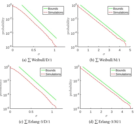
Figs. 1.(a-d) illustrate upper bounds vs. simulations for the CCDF

of the waiting time in heavy-traffic (ρ=0.99). In the Erlang-k case, λ:=√2k

π such thatE

T1,1

is the same as in the Weibull case. The

simulations are obtained from 107samples, each representing the

waiting time of the 105th job starting from an empty system. The

tail instability is due to the simulation length; note thatΘ 1012

0 10 20 30 40 10-6

10-4 10-2 100

Bounds Simulations

(a)ÍWeibull/D/1

0 50 100 150

10-6

10-4 10-2 100

Bounds Simulations

(b)ÍWeibull/M/1

0 10 20 30 40

10-6

10-4 10-2

100

Bounds Simulations

(c)ÍErlang-3/D/1

0 50 100 150

10-6

10-4 10-2 100

Bounds Simulations

(d)ÍErlang-3/M/1

Figure 1: Waiting-time CCDF (upper bounds vs. simula-tions); (N=5,ρ=0.99)

intervals. Besides the accuracy of the bounds, an interesting

obser-vation is that in the case of constant service times, the inter-arrival

distribution makes a substantial difference on waiting times; this

effect disappears however in the case of exponential service times.

Appendix § B provides additional simulations (Fig. 9) illustrating

that the bounds degrade at lower utilizations, and especially for

constant service times.

The issue of the bounds’ tightness is closely related to the

es-timation of theovershoot. Having a (Markov) random walk with

increments(Ui)i, and a valueσ ≥0, the overshoot is defined as

Rσ =inf{U1+U2+· · ·+Un−σ |U1+U2+· · ·+Un ≥σ}.

In the proof of Theorem 7, the derivation of the bounds mainly

relies on the crude estimationRσ ≥ 0; see also the discussion around Lemma 2. Without resorting on a rigorous argument, we

believe that in heavy-traffic the last increment behaves as a

typ-ical increment, whereas in lower-traffic the last increment gets

larger; ignoring this information is a possible cause for the bounds

degradation. For potential improvements of the crude overshoot

estimation see Chang [11].

4.3

Example 3:

Σ

Weibull

+

Σ

Erlang-

k

/G/1

Let us now consider a heterogeneous mix ofN1Weibull andN2

Erlang-k classes, mutually independent. We use the same

parame-ters as before, includingλ:=√2k

π in the Erlang-k case, to

normal-ize the arrival rates of the two classes. The service times satisfy E[S1,1]=_λNk ρwhereN :=N1+N2andρis the overall utilization.

Denote the Weibull and Erlang-k compound processes asAi(t)for i=1. . .N1andi=N1+1, . . . ,N, respectively.

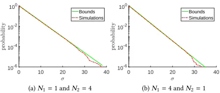
We next illustrate the algorithm for computing a waiting time

bound in the case of heterogeneous input. Recall the key idea

from § 3.2 of obtaining martingales with the same ‘θ’ for both

classes (in this caseN1Weibull and N2 Erlang-k), and also the

0 10 20 30 40

10-6 10-4 10-2 100

Bounds Simulations

(a)N1=1 andN2=4

0 10 20 30 40

10-6 10-4 10-2 100

Bounds Simulations

(b)N1=4 andN2=1

Figure 2: Waiting-time CCDF for a Weibull job;N1Weibull

andN2Erlang-k classes; constant (D) service times; (N =5, k=3,ρ=0.99)

proofs of Corollaries 9 and 10. We thus look for a split

w1N1+w2N2=N

which yields the martingales

hW(R1(t))e

θ1_wN 1(A1

(t)−w1

Nt)

for a single Weibull compound processA1(t)and

hE(RN1+1(t))e θ2_wN

2(AN1+1(t)−

w2

Nt)

for a single Erlang-k compound processA2(t); the ‘W’ and ‘E’

sub-scripts correspond to the two classes.

The same ‘θ’ constraint reduces to

θ:=θ

1N w1

=θ2N

w2 .

We also note the additional constraints onw1andw2to guarantee

the existence of the two martingales above

ρ <w1<

N−N2ρ N1

,

which are merely stability conditions (e.g., the rate ofA1(t)is less

thanw1

N). The existence ofw1satisfying the same ‘θ’ constraint is

guaranteed by the continuity off₁(w₁):=θ1N w1

andf₂(w₁):=θ2N w2 ,

and the extreme pointsf1(ρ)=0 (because the correspondingθ1is

zero) andf2(

N−N2ρ N1

)=0.

MultiplexingN1Weibull classes andN2Erlang-k classes yields

the martingale

N1 Ö

i=1

hW(Ri(t)) N

Ö

i=N1+1

hE(Ri(t))eθ(A(t)−t)

whereA(t):=ÍN_i

=1Ai(t)is the overall compound process.

There-fore, a bound on the waiting-time of a Weibull class is

P(W ≥σ) ≤KW(θ)N1−1K

E(θ)N2e−θ σ,

whereK_W(θ)andK_E(θ)are theK(θ)’s from Corollaries 9 and 10,

respectively. In turn, the waiting time of an Erlang-k class is the

same except for the prefactorK_W(θ)N1K E(θ)N2−1

.

We illustrate the accuracy of these bounds for aΣWeibull+

ΣErlang-k/D/1 queue in Fig. 2; both cases of disproportionate Weibull and Erlang-k classes relative to the other are addressed in (a) and

(b). The numerical settings are the same as in Fig. 1. Results with

shown here), whereas the accuracy of the bounds degrade at lower

utilization (similar as in Fig. 9 from Appendix § B).

5

APPLICATION 2: QUEUES WITH

MARKOVIAN ARRIVALS

We now apply Lemma 5 to several subclasses of MAPs from

tele-traffic theory: Markov Modulated Fluid (MMF, § 5.1), Markov

Mod-ulated Poisson Process (MMPP, § 5.2), and (Generalized) Markovian

Arrival Processes ((G)MArP, § 5.3).

0 P

µ

λ P

Figure 3: MMOO process

5.1

Fluid Scenario. MMF

The MMF model assumes that data is infinitely divisible (i.e., a

continuous ‘fluid’), whereas a background processM_tdetermines

the rate at which the fluid arrives at the server:

A(t)=

∫ t

0

Msds. (12)

In the basic Markov-Modulated On-Off (MMOO) model [2],M_thas

two states (denoted for convenience 0 andP) with transition rates λandµ(see Fig. 3). While in state 0 (also referred to as ‘off ’) the process does not generate any fluid; while in stateP(also referred

to as ‘on’) the process generates ‘fluid’ at some constant rateP.

Before applying Lemma 5, we remark that the parameterChas

the meaning of the rate of a hypothetical queueing server for the

processA(t). To avoid trivial situations we assume thatP>C(i.e.,

the peak rate is greater than the capacity) and that the utilization

factorρ=

µ λ+µP

C satisfies the stability conditionρ<1.

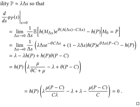
Corollary 11. (Single MMOO)In the scenario above, let

θ:= λ P−C −

µ

C , h(P):= θC+µ

µ , and h(0):=1. Then the process

h(Mt)eθ(A(t)−Ct)

is a martingale.

Proof. We distinguish two cases. First, ifM0 = 0, then in a

small interval[0,∆s]the processM_s jumps to the ‘on’-state with probability_P≈µ∆s(more precisely_P=µ∆s+o(∆s)). We have

d dsφ0(s)

_s=

0

= lim

∆s→0

1

∆sE

h

h(M_∆s)eθ(A(∆s)−C∆s)−h(0) M0=0

i

= lim

∆s→0

1

∆s

µ∆sh(P)eθ∆s(P−C)+(1−µ∆s)e−θC∆s−1

=µh(P) −µ−θC=0,

after applying Taylor’s expansionex∆s =1+x∆s+o(∆s). Similarly, ifM0=Pthen the process jumps in[0,∆s]with

prob-ability_P≈λ∆sso that

d dsφP(s)

_s=0

= lim

∆s→0

1

∆sE

h

h(M∆s)eθ(A(∆s)−C∆s)−h(P)

M0=P

i

= lim

∆s→0

1

∆s

λ∆se−θC∆s+(1−λ∆s)h(P)eθ∆s(P−C)−h(P)

=λ−λh(P)+h(P)θ(P−C)

=h(P)

λ µ

θC+µ−λ+θ(P−C)

=h(P)

λµ(P−C)

Cλ −λ+λ−

µ(P−C)

C

=0.

The MMOO martingale appeared in a general form for Markov

fluids in Ethier and Kurtz [21] (see Lemma 3.2 therein), which was

instantiated in the MMOO case by Palmowski and Rolski [40]. Note

that Corollary 11 not only provides an elementary proof, but it also

guarantees the unicity of exponential martingales of the form from

Eq. (9) for the MMOO process (subject to a fixedC).

Next we consider an aggregate ofN MMOO processes

repre-sented in Fig. 4. The corresponding aggregate process isA(t)and

the background process withN +1 states isMt; the utilization

factorρ =

µ λ+µP N

C satisfiesρ<1.

0 P 2P . . . N P

N µ

λ

(N−1)µ

2λ

µ

N λ

P 2P N P

Figure 4: An aggregate ofN MMOO processes

Corollary 12. (Multiplexed MMOO)In the scenario above, let

θ=N_C

_λC

N P−C −µ

,h(iP)=

1+Cθ N µ

i

i=0, . . . ,N.

Then the process

h(Mt)eθ(A(t)−Ct)

is a martingale.

Bounds on the waiting time distribution follow directly from

Theorem 7. Denoting for conveniencec:= C_N andb:=1+cθ_µ we

have

P(W ≥σ) ≤ ÍN

i=0πib

i

bPc e

whereπ_i = N_{i µ}

λ+µ

i _λ

λ+µ

N−i

are the stationary probabilities

ofM_t. We deliberately used the weaker bound withb

c

P, instead of b⌈c_P⌉

, which lends itself to the ‘expressive’ bound from [15]

P(W ≥σ) ≤KNe−θ σ , (13)

whereK:=ρ _ρ−p

on 1−p_on

pon_ρ −1

<1 andp_on:= µ

λ+µ; the same bound appeared in [40] yet without the explicit exponential representation

of the prefactor. We also note that in the application of Theorem 7

we have Im(Mt)={⌈_Pc⌉, . . . ,N}because at least⌈_Pc⌉individual sources must be ‘on’ to guaranteea(T) ≥Cat the stopping time T; the rest follows from the monotonicity ofh(iP). The bounds from (13) are accurate, at both high (ρ =.9) and moderate (ρ = .75) utilizations, as illustrated through simulations in [15]. The fundamental reason is that the bound from (13) captures the right

scaling inN, as conjectured by Choudhuryet al.[13].

5.2

Packet Scenario. MMPP

Here we analyze the ‘packetized’ version of the MMF model; we

consider both constant and random packet sizes.

5.2.1 Constant Packet Size.Data consists of indivisible units (i.e., ‘packets’) of size 1. The instantaneous probability of a packet

arrival is determined by a background processM_t, whereas the

cumulative arrivals processA(t)evolves according to

P(A(t+∆t) −A(t)=1)=r(Mt)∆t+o(∆t), (14)

wherer(·)is a rate function. For instance, we letMtbe the Markov process from Fig. 5a, i.e., state space{1,2}and transition ratesµ1

andµ₂, in which caser(1)=λ₁andr(2)=λ₂.

1 2

µ1

µ2

λ1 λ2

(a)

1 2

p

1−p

q

1−q

Exp_ξ 1

Exp_ξ 2

(b)

Figure 5: MMPP (a) and packet size modulator (b)

To construct a martingale fromA(t)using Lemma 5 we need the following matrix transform: Forθ >0, let

Tθ := _λ

1eθ−µ1−λ1 µ1

µ2 λ2eθ −µ2−λ2

and denote byλ(θ)its spectral radius.

Corollary 13. In the scenario above, pickθ>0such thatλ(θ)= θC, and leth=(h1,h2)be an eigenvector corresponding toTθ and λ(θ). Then the process

h(M_t)eθ(A(t)−Ct)

is a martingale; for notation’s convenienceh(i) ≡h_i.

We next apply Theorem 7 in the case of N multiplexed

(homoge-neous) MMPPsA_i(t), with background processesM_i,t, served at

rateC, and utilizationρ<1. Letting the individual martingales

h(Mi,t)eθ

Ai(t)−C_Nt

withh(·)andθ as in Corollary 13 (withC replaced by C_N), the aggregate martingale is

Ö

i

h(Mi,t)eθ(ÍiAi(t)−Ct)_.

We then obtain the following upper bound on the waiting time

P(W ≥σ) ≤ E_h

(M1,0)

N

min{h1,h2}N

e−θCσ . (15)

Assuming that the system is initially stationary,Eh(M_1,0) = h1

µ2 µ1+µ2+h2

µ1 µ1+µ2

. The lower bound is similar except for replacing

the ‘min’ by ‘max’, andσbyσ+1 (as packets have size 1).

5.2.2 Random Packet Size.We extend the previous model from constant to random packet sizes. We assume that a Markov chain Lndetermines the size of then-th packet. The chainL_nalternates between two states with transition probabilitiespandqas in Fig. 5b.

The packets are exponentially distributed with ratesξ1andξ2

de-pending on the chain’s state; other types of distributions can be

considered. Note that in the caseξ1=ξ2we have the scenario with

i.i.d. packet sizes.

IfA(t)is the cumulative arrival process with constant packet

sizes (as in Subsection § 5.2.1), the arrival process with random

packetsArnd(t)has the representation

Arnd

(t):=

A(t)

Õ

k=1 SLk,k,

where(S_1,k)_k∈

Nand(S2,k)k∈_Nare i.i.d. sequences of exponential

random variables with ratesξ1andξ2, respectively. Note that the

process

Arnd

(t),

Mt,LA(t)

is a MAP in the sense of Definition 4.

In order to apply Lemma 5 to this example, we need the following

matrix transformT_θ forθ >0

T_θ := © ­ ­ ­

«

(1−p)λ1Eeθ S1,1−µ1−λ1 pλ1Eeθ S2,1 µ1 0

qλ1Eeθ S1,1 (1−q)λ1Eeθ S2,1−µ1−λ1 0 µ1 µ2 0 (1−p)λ2Eeθ S1,1−µ2−λ2 pλ2Eeθ S2,1

0 µ2 qλ2Eeθ S1,1 (1−q)λ2Eeθ S2,1−µ2−λ2

ª ® ® ® ®

0 50 100 150 200 10-1

100

Upper/Lower Bounds Simulations

(a) constant

0 50 100 150 200

10-1 100

Bounds Simulations

(b) random

Figure 6: Waiting-time CCDF forN MMPPs; constant and random packet sizes; (N =5,µ1=0.1,µ2=0.5,λ1=1,λ2=25, p=0.1,q=0.9,E[ξ1]=0.2,ρ=0.99)

Letλ(θ)be its spectral radius.

Corollary 14. In the scenario above, pickθ>0such thatλ(θ)= θC, and leth= h1,1,h1,2,h2,1,h2,2

be an eigenvector corresponding toTθ andλ(θ). Then the process

h(Mt)eθ

Arnd_(t)−Ct

is a martingale.

An upper bound on the waiting time is the same as in Eq. (15)

except for the denominator in the prefactor, which is replaced by

min{h1,1,h1,2,h2,1,h2,2}N according to Corollary 14. In turn, a

lower bound cannot be obtained with Theorem 7 because packet

sizes are unbounded.

Figure 6 illustrates the accuracy of the bounds in the case of an

aggregate of MMPP flows in heavy-traffic (ρ =0.99). Both cases

of constant and random-size packets are considered; in both cases

the upper bound and simulation lines almost overlap, the former

being slightly above the other. Simulations are obtained from a run

of 1010packets of which the first 10% were discarded. Additional

simulations for smaller utilizationρ=0.75 are shown in Figure 10

in Appendix § B.

5.3

Packet Scenario. MArP and GMArP

As in the MMPP case we address both constant and random packet

sizes.

5.3.1 Constant Packet Size. First we consider Markovian Arrival Processes (MArPs) that generalize the Markov Modulated Poisson

processes from § 5.2.1.

Definition 15. A Markovian Arrival Process is defined via a pair

(D0,D1)ofn×n-matrices such that: di,j :=D0(i,j) ≥0,i,j, d

′

i,j:=D1(i,j) ≥0, di,i :=D₀(i,i)=−

Õ

i,j

di,j−Õ j

d′ i,j .

The background processMtis a Markov process with generatorD0+D1 and steady-state distributionπ. If a transition ofMtis triggered by an element ofD1, a packet is generated andA(t)increases by1(active

transitions); transitions triggered byD0do not increaseA(t)(hidden

transitions):

P(A(t,t+∆t)=0,M_t+∆t =j |M_t=i)=D0(i,j)∆t+o(∆t),

and

P(A(t,t+∆t)=1,M_t+∆t =j |M_t=i)=D₁(i,j)∆t+o(∆t). Corollary 16. In the scenario above, forθ >0, letλ(θ)be the spectral radius of the matrix

D0+eθD1.

Ifλ(θ)=θCandhis a corresponding eigenvector then the process

h(Mt)eθ(A(t)−Ct) (16) is a martingale. Moreover, ifhris an eigenvector corresponding to the spectral radius of the transform matrix

Π−1

D0+eθD1

T

Π,

whereΠis the matrix with the steady state distributionπ on its diagonal, then the process

hr(Mr_t)eθ(Ar(t)−Ct)

is a martingale as well.

An immediate consequence of the second part of the Corollary

is that in the general case of not necessarily reversible processes,

an upper bound on the waiting time is the same as in (15), except

for accounting for the "reversed" eigenvectorhr.

A key property of MArPs is their stability under superposition:

Given two MArPs(A(t),M_t)and(A′(t),M_t′)with corresponding matrices(D₀,D₁)and(D′

0,D

′

1), respectively, the aggregate arrival

processA(t)+A′(t)is a MArP with matrices

(D0⊕D

′

0,D1⊕D

′

1),

where ‘⊕’ stands for the Kronecker sum. The next result gives the resulting martingale:

Corollary 17. In the situation with two MArPs as above, for θ >0, letλ(θ)andλ′(θ)denote the spectral radii of the matrices

D0+eθD1andD

′

0+e

θ_D′

1,

respectively; let alsohandh′be the corresponding eigenvectors. If λ(θ)+λ′(θ)=θCthen the process

h(Mt)h′(M_t′)eθ(A(t)+A′(t)−Ct)

is a martingale.

The result generalizes immediately to any number of MArPs.

5.3.2 Random Packet Size.We finally consider Generalized Mar-kovian Arrival Processes (GMArPs) that generalize the MArPs

from § 5.3.1 by allowing for random packet sizes.

Definition 18. A Generalized Markovian Arrival Process (GMArP)

is defined via a sequence(L_k)1≤k<∞of strictly positive distributions and a sequence(D_k)0≤k<∞ofn×n-matrices such that

Dk(i,j) ≥0,i_,j, for allk≥0, and

D0(i,i)=−

Õ

i,j

D0(i,j) −

∞

Õ

k=1

Õ

j

Dk(i,j).

The background processMtis a Markov process with generatorÍ∞

byL_k. Accordingly,A(t)increases byXk, i.e., a random variable independently drawn from the distributionL_k.

If in the above definition we letD_k:=0 for allk≥2, andL1:= δ1, i.e., the deterministic distribution on 1, we recover the MArP

scenario from the previous section. Moreover, if onlyL_k :=δ_k, i.e., the deterministic distribution onk, GMArP instantiates to the

Batch Markovian Arrival Process (BMArP) [37].

Corollary 19. In the scenario above, forθ >0, letλ(θ)denote the spectral radius of the matrix

∞

Õ

k=0

E[eθ Xk]Dk.

Ifλ(θ)=θC, andhis a corresponding eigenvector, then the process h(M_t)eθ(A(t)−Ct)

is a martingale. Moreover, ifhr is an eigenvector corresponding to the spectral radius of the transposed matrix

Π−1

∞

Õ

k=0

E[eθ Xk]Dk

!T

Π,

whereΠdenotes the matrix with the steady state distributionπon its diagonal, then the process

hr(M_tr)eθ(Ar(t)−Ct)

is a martingale as well.

Proof. Analogously to the proof of Corollary 16.

We also note that multiplexing GMArPs can be treated in the

same manner as in Corollary 17, whereas a bound on the waiting

time follows exactly as in the MArP case.

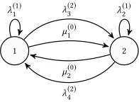
1 2

µ(0)

1 λ(2)

3 λ(1)

1

µ(0)

2 λ(2)

4

λ(1)

2

Figure 7: Example of GMArP

To provide numerical results we consider the GMarP process

from Fig. 7. By convention, the superscript in each transition

corre-sponds to the ‘k’ from Def. 18. More precisely

D0=

−λ1−λ3−µ1 µ1 µ2 −λ2−λ4−µ2

D1=

λ1 0

0 λ2

, D2=

0 λ3 λ4 0

.

Note that unlikeλ1andλ2, the transitionsλ3andλ4involve a

change of state, in addition to drawing a packet size from a different

distribution.

In Fig. 8 we consider an aggregate ofN = 5 homogeneous

GMArPs, and both constant and exponential packet sizes. The

nu-merical settings normalize the average rate as in the MMPP case

0 50 100

10-4 10-2 100

(a) constant

0 50 100

10-4 10-2 100

Bounds Simulations

(b) random

Figure 8: Waiting-time CCDF forN GMArPs; constant and random packet sizes; (N = 5,µ1 = 0.1,µ2 = 0.5,λ1 = 0.3, λ2=10,λ3=0.7,λ4=15,E[X1]=1,E[X2]=3.01,ρ=0.99)

(Fig. 6); however, we now consider much burstier processes.

Sim-ulations are run as in the MMPP case; similarly, the upper bound

and simulation lines almost overlap.

Let us now comment on the numerical complexity in analyzing

queues with a superposition ofNBMArP. The standard approach

consists in computing the generator matrix of the superposed

pro-cess, which has an exponential number of states (inN) as a

conse-quence of the Kronecker product. Exact results (e.g., on the waiting

time distribution) can be obtained by applying a mix of

matrix-analytic techniques and inversion algorithms of Laplace transforms

(for an overview see [37]). A computationally more effective

ap-proach in the case of MArPs consists in building a n-dimensional

Markov process, where n is the number of states for each (i.i.d.)

MArP; the overall number of states is N+n−1

n−1

which is generally

much smaller than the exponential. This approach has its roots

in the analysis of GI/PH/N queues [43]; for a discussion of the

applications of this approach, including queues with superposed

MArPs, see [24]. In turn, bounding approaches as in this paper or

the literature (e.g., [9, 36]) are subject to a linear complexity.

6

DISCUSSION

Here we discuss some related work in more detail and comment on

possible extensions of our results.

6.1

Related Work

Kingman’s GI/G/1 bound from (4) was extended to the case of

discrete-timeMAPs in Chang and Cheng [10]. Using a different martingale transform, Duffield [18] improved the bounds by

essen-tially capturing the positiveness of the instantaneous drift at the

underlying stopping time (this fact holds by default in the renewal

case and does not have to be properly accounted for). This

improve-ment can be substantial because in some cases, e.g., bursty On-Off

processes whereby the sum of the transition probabilities between

the two states is less than 1, the prefactor in the exponential bound

is also less than 1; in turn, the prefactor from [10] is always greater

or equal than 1. Another martingale transform was constructed

by Fanget al.[22] using a fixed point argument in the case of the

G/GI/1 queue, allowing for Markovian inter-arrivals; while there

is similarity to Duffield’s approach (which essentially relies on the

eigenvalue/eigenvector problem – a fixed point problem itself ), a

qualitative comparison is challenging due to the different bounds’

In a more recent work, Jiang and Misra [29] obtained bounds in

ΣGI/G/1 queues. In theΣD/D/1 case, tight worst-case bounds are obtained by relying on network calculus models and techniques.

The general case is treated by discretizing time and then directly

applying Kingman’s technique, as outlined in § 2. A proof for the

claimed discrete-time martingale is however not given, and we

believe that it may be challenging due to the loss of the renewal

property in the general case. For Poisson arrivals, the renewal

property is preserved under superposition and the martingale

con-struction holds; the obtained bounds—which are essentially the

same as in this work, as well as in [30] by properly instantiating

the general results—are shown to be numerically accurate.

Kingman also provided a more powerful GI/G/1 bound in [31].

In the notation from § 2.1

P(W ≥σ) ≤γ(σ),

whereγ(σ)is a non-increasing function with 0≤γ(σ) ≤1 such

that for allσ>0

∫ σ

−∞

γ(σ−y)dF(y)+1−F(σ) ≤γ(σ), (17)

whereF(y)is the distribution ofU1. The bound facilitates the

dis-covery of tighter bounds than the original bound from (4), which is

recovered withγ(σ):=e−θ σ.

This idea was exploited by Liu, Nain, and Towsley [35, 36] in

the case of general discrete-time MAPs, whereby the background

Markov chain can have a general state space. The method extends

immediately to continuous-time MAPs by embedding a Markov

chain to account for the the (discrete-time) structure of the integral

inequality from (17). Notably, the obtained bounds areexactfor the

GI/M/1 queue, which also holds for Ross’ bounds from [46] (see (7));

based on this match, it is of interest to qualitatively compare the

bounds from [36, 46] (see the proof of Lemma 3 for the extension

of Ross bounds to the non-renewal case).

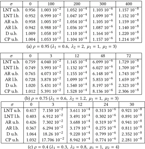
Such a qualitative comparison is provided in [35, 36] for the

bounds therein and those from [18], and also from Asmussen and

Rolski [5]; the latter are derived in the context of risk theory (for

the analogy between ruin probabilities and tail bounds on waiting

time see [3]). A deep comparison is however very challenging due

to the different structures of the bounds. Numerical comparison

between the three bounds (and also some corresponding lower

bounds) are given in [36]; we reproduce some tables in

Appen-dix § B (see Figs. (12) and (13), and include our bounds from § 5.2.1

for the MMPP/D/1 queue (see (15)) and § 5.2.2 for the MMPP/M/1

queue; we refer to our bounds as CP (the authors’ initials), and to

the other three similarly (LNT-Liu/Nain/Towsley, D-Duffield, and

AR-Asmussen/Rolski). In the MMPP/D/1 case the CP-bounds are

essentially identical to the AR-bounds. In the MMPP/M/1 case the

CP-bounds are only slightly better than the D-bounds, which were

identified in [36] as the loosest for the numerical settings therein.

From a qualitative point of view, the CP-bounds are most ‘similar’

to the D-bounds. The fundamental difference is that the CP-bounds

are derived exclusively in time, using a

continuous-martingale, whereas the D-bounds are derived in discrete-time but

using the same technique from Theorem 7 extending Kingman’s

original idea to the non-renewal case. A slight difference is that the

CP-bounds hold for the virtual delay process whereas the D-bounds

hold for the packet delay; a normalization between the two

mea-sures can be obtained using a Palm argument (see Shakkottai and

Srikant [47]). There is also a deeper difference in that continuous

and discrete-time models (e.g., Markov On-Off processes/chains)

can lend themselves to qualitatively different bounds (see the

expo-nential decay with prefactor less than 1 from (13); the same holds

in the case of an On-Off chain but under a specific burstiness

con-dition on the transition probabilities, see Buffet and Duffield [8],

which is the same as the embeddability condition of Markov chains

in Markov processes, see Poloczek and Ciucu [41]).

The CP-bounds (reproduced from [15]) are almost identical to

those from Palmowski and Rolski [40] in the case of the

continuous-time Markovian fluid; only the MMOO model was considered

in § 5.1 due to its expressiveness. As in Theorem 7, [40] exclusively

works in continuous-time using a continuous-time martingale from

Ethier and Kurtz [21]. Unlike the MMOO case, the general case

from [40] appears to miss the fundamental improvement of the

bounds related to the property of the instantaneous increment at

the stopping time; this likely overlook was rectified by Ciucuet

al.[16].

6.2

Extensions

The results in this paper assume a constant-rate service rate; even

the GI/G/1 queue was treated by constructing a compound arrival

process to be served at rate one. The underlying principle behind

this approach is to encodeallthe information about arrivals,

in-cluding the service times of packets in the GI/G/1 case, in a single

model, i.e., the martingale representation; this model is referred to

in Poloczek and Ciucu [42] as anarrival-martingale.

A fundamental motivation of this approach, which essentially

follows from the network calculus principles (see Chang [9], Le

Boudec and Thiran [7], and Jiang and Liu [28]), is to decouple

arrivals from service. One key benefit is the straightforward

ex-tension to random service rates, by encodingallthe information

about service in aservice-martingale[42] (defined therein for some

(discrete-time) Markov-modulated processes modelling specific

wireless channels). In our context, we can represent service in

terms of a MAP(S(t),Lt)tand slightly change Lemmas 5, 6 to con-struct service-martingales in the homogeneous or inhomogeneous

cases. The main difference is a sign-change in the exponential of

the martingale, i.e.,

h(Lt)e−θ(S(t)−Ct).

(a service-martingale essentially extends an arrival-martingale in

the same way that effective-capacity (Wu and Negi [51]) extends

effective bandwidth).

Given an arrival-martingaleha(Mt)eθa(A(t)−Cat)and a

service-martingaleh_s(L_t)e−θs(A(t)−Cst), the bounds from Theorem 7

ex-tend easily.CaandC_bshould be selected such thatθa =θs =:θ, using the algorithm from § 4.3; existence is again guaranteed from

stability. A backlog upper bound is then

P(Q≥σ) ≤ E

[ha(M0)]E[hs(L0)]

max_(m,l)∈Dh_a(m)h_s(l)e

−θ σ _{, (18)}

whereD={(m,l) |∃t:M_t =m∧L_t =l∧a(t) ≥s(t)}(s(t)is the

instantaneous service, i.e.,S(t)= ∫t

0 s(u)du