Salient object detection employing robust sparse
representation and local consistency
Yi Liua,b, Qiang Zhanga,b,∗, Jungong Hanc, Long Wangd
aKey Laboratory of Electronic Equipment Structure Design, Ministry of Education, Xidian
University, Xi’an Shaanxi 710071,China
bCenter for Complex Systems, School of Mechano-Electronic Engineering, Xidian
University, Xi’an Shaanxi 710071,China
cDepartment of Computer Sciences and Digital Technologies, Northumbria University,
Newcastle upon Tyne NE1 8ST, U.K
dCenter for Systems and Control, College of Engineering, Peking University, Beijing
100871, China
Abstract
Many sparse representation (SR) based salient object detection methods have
been presented in the past few years. Given a background dictionary, these
methods usually detect the saliency by measuring the reconstruction errors,
leading to the failure in the complex scene. In this paper, we propose to replace
the traditional SR model with arobust sparse representation (RSR) model, for
salient object detection, which replaces the least squared errors by the sparse
errors. Such a change dramatically improves the robustness of the saliency
de-tection in the existence of non-Gaussian noise, which is the case in most practical
applications. By virtual of RSR, salient objects can equivalently be viewed as
the sparse but strong “outliers” within an image so that the salient object
de-tection problem is reformulated to a sparsity pursuit one. Moreover, we jointly
utilize the representation coefficients and the reconstruction errors to
construc-t construc-the saliency measure in construc-the proposed meconstruc-thod. Finally, we inconstruc-tegraconstruc-te a local
consistency prior among spatially adjacent regions into the RSR model in order
to uniformly highlight the whole salient object. Experimental results
demon-strate that the proposed method significantly outperforms the traditional SR
based methods and is competitive with some current state-of-the-art methods,
especially for those images with complex structures.
Keywords: Salient object detection, robust sparse representation, local
consistency, complex structures
1. Introduction
Visual saliency refers to identifying certain regions of a scene, which stand
out from their surroundings and catch immediate attention [1]. As an important
branch of visual saliency, salient object detection has attracted a wide range of
attention. Generally, it is essentially a binary segmentation problem [2] starting
5
by detecting the attractive objects in a scene followed by a segmentation
proce-dure that extracts the entire objects from the background. It has been widely
applied to many fields, such as image segmentation [3], classification [4], cluster
[5], recognition [6], content-based image retrieval [7] and image fusion [8].
Recently, sparse representation (SR) has been exploited to salient object
de-10
tection [9, 10, 11, 12] as a result of its successful applications in many computer
vision and image processing tasks, such as face recognition [13], image
classifi-cation [14], and so on. In these SR based methods, the salient object detection
is normally carried out in three steps. First, input images are divided into many
patches or super-pixels. Secondly, an over-complete dictionary is constructed,
15
which helps to encode the feature vectors collected from those patches or
super-pixels. Thirdly, the saliency value for each patch or super-pixel is measured
according to its representation coefficients or residual errors.
For the SR based salient object detection methods, there are two important
issues: dictionary construction and saliency measure. Earlier methods are prone
20
to adopt the surrounding patches of each test patch as the dictionary [9, 10].
Due to the fact that the edges of salient objects have high contrast against
their surrounding patches, such SR based methods usually assign higher salient
values to the edges rather than the whole objects, as illustrated in Fig. 1(b).
Recently, some boundary priors [15] are integrated into these methods based on
the assumption that backgrounds are usually distributed on the boundary of an
image. Under this assumption, the patches or super-pixels near the boundary
of an image are often selected to construct a background dictionary [12, 16, 17].
As shown in the first row of Fig. 1(c), these methods could overcome the
shortcomings of those methods with the surrounding patches as the dictionary.
[image:3.612.156.452.215.436.2]30
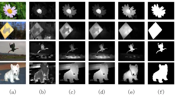
Figure 1: Typical challenging examples for SR based salient object detection methods. (a)
Original images; (b) SR based method with surrounding patches as the dictionary [10]; (c)
SR based method with background templates near the image boundary as the background
dictionary; (d) Proposed RSR method with the background dictionary but without the local
consistency prior; (e) Proposed RSR method with the background dictionary as well as the
local consistency prior; (f) Ground truth.
With respect to the saliency measure, most SR based salient object detection
methods employ either the sparseness (i.e., the coding length) of the
representa-tion coefficients or the reconstrucrepresenta-tion errors, especially the latter, to define the
saliency measure [9, 10, 11], because there is an assumption that natural signals
can be represented or approximately represented as a linear combination of a
35
“few” atoms from a redundant dictionary [9, 10].
detec-tion methods imposes a sparsity constraint on the representadetec-tion coefficients
to achieve the sparse coding of each test image patch or super-pixel. It
ba-sically minimizes the sum of squared reconstruction errors, therefore tending
40
to be sensitive to the non-Gaussian noise as well as sparse “outliers” [13, 18].
Two undesirable results will be obtained when the residual errors are used as
the saliency measure, especially for those methods based on the background
dictionary. One is that many regions belonging to the foreground will not be
highlighted when the foreground object and the background look similar, as
45
shown in the second and third rows in Fig. 1(c). The other one is that the
background will not be well suppressed, as shown in the last two rows in Fig.
1(c).
Moreover, there generally exist strong spatial correlations among the local
regions in an image, i.e., the spatially adjacent patches or super-pixels with
50
similar features should have similar saliency values. But in most of the existing
salient object detection methods, this local consistency is often ignored, and the
saliency of each image patch or super-pixel is computed independently. As a
result, the whole salient object could not be uniformly highlighted, as shown
in the third and last rows in Fig. 1(d). Besides, background can not be well
55
suppressed, resulting parts of the background being falsely taken as the salient
regions, as shown in the first and fourth rows in Fig. 1(d).
In this paper, we aim to detect the salient object in an image with complex
structures by addressing the two problems mentioned above. More specifically,
to enhance the algorithm robustness against the non-Gaussian noise, we replace
60
the least squared reconstruction errors with the sparse reconstruction errors.
In another word, we impose al2,1-norm minimization constraint on the
recon-struction errors to ensure the column-sparsity of the error matrix. It can be
interpreted as that the salient objects are sparsely distributed “outliers” within
an image and seeking such “outliers” is equivalent to a sparsity pursuit
prob-65
lem, which can be solved by a robust sparse representation (RSR) model [18].
When applied to the detection of salient objects, RSR is expected to possess
as shown in Fig. 1(d). Besides, based on the local consistency, the spatially
ad-jacent pathes or super-pixels with similar features should have similar saliency
70
values. Thus they should possess similar sparse representation coefficients as
well as reconstruction errors when they are sparsely coded by using RSR with
respect to the same background dictionary. We achieve that by introducing
t-wo Laplacian regularizations with respect to the representation coefficients and
reconstruction errors, respectively, into the RSR model. As a result, the whole
75
salient object can be uniformly highlighted and the background can also be well
suppressed, a shown in Fig. 1(e). Eventually, an object function taking both
the above mentioned aspects into account is minimized, thus helping to generate
the saliency map.
In summary, our paper differs from the existing works in three aspects:
80
(1) We employ the RSR model, instead of the traditional SR model, in our
proposed method. To our best knowledge, this is the first attempt to apply
the RSR model to the detection of salient objects. By virtue of RSR, the
salient object is modeled as sparse but strong “outliers” within an image so that
the salient object detection can be accomplished by solving a sparsity pursuit
85
problem.
(2) We involve a local consistency prior among spatially adjacent regions by
imposing two Laplacian regularizations on the representation coefficients and
reconstruction errors in our proposed method. This is different from the existing
method in [17], in which only a Laplacian regularization term is imposed on the
90
representation coefficients.
(3) Two saliency measures are defined based on the representation
coeffi-cients and the reconstruction errors, respectively, and the two saliency measures
are fused to obtain the final saliency measure. Especially, in the representation
coefficient based saliency measure, the sparseness and magnitude information
95
of the representation coefficientsare jointly employed.
The remainder of this paper is organized as follows. Section 2 briefly reviews
the related work. Section 3 describes the proposed salient object detection
and Section 5, respectively.
100
2. Related work
2.1. Contrast-based salient object detection methods
During the last few years, numerous salient object detection methods have
been proposed [9, 10, 11, 12, 19, 20, 21, 22, 23, 24, 25, 26, 27, 28], among which
the contrast-based methods are most popular [9, 10, 15, 16, 21, 22, 26, 27].
105
These contrast-based methods can be further divided into local-contrast based
and global-contrast based ones, respectively.
Local-contrast based methods tend to highlight a certain region with high
visual attention with respect to its small neighborhoods [17, 21, 22, 29]. The
earlier local-contrast based methods are designed for only saliency detection
110
[19], but in recent years, they are extended to salient object detection [21, 29].
The common observation is that these methods tend to produce higher saliency
values near the edges instead of uniformly highlighting the whole salient objects.
As opposed to those local-contrast based ones, global-contrast based
meth-ods evaluate the saliency value of each pixel or region with respect to the entire
115
image [22, 23]. In other words, these methods aim to capture the holistic rarity
or uniqueness from an image. Compared with the local-contrast based methods,
global-contrast based methods can obtain more uniform detection results and
have attracted more attentions [20, 22, 23].
In view of the advantages of local-contrast based and global-contrast based
120
methods, combining such two methods has been studied in recent years [24, 25,
30, 31]. For example, in [24], a salient object detection method was presented,
which integrated a global saliency estimation via a high-dimensional color
trans-form (HDCT) and a local saliency estimation via regression. The two resulting
saliency maps complemented each other to obtain a final saliency map.
Similar-125
ly, in [25], the authors presented a coding-based saliency measure by exploring
2.2. SR based salient object detection methods
Recently, some salient object detection methods have been presented based
on the sparse representation (SR) theory. In the earlier SR based methods, the
130
predefined dictionary is simply selected from the surrounding patches of each
given test patch. Such approaches generally produce higher saliency values at
the boundaries of the object [9, 10]. In essence, these methods can be categorized
as the local-contrast based ones.
Lately, several boundary priors [15] have been integrated into these SR based
135
methods considering the fact that the background is usually distributed on the
boundary of an image. Based on this assumption, the patches or super-pixels
near the image boundary are often selected to construct a global background
dictionary. Then, the saliency value for each patch or super-pixel could be
mea-sured according to reconstruction errors with respect to the predefined
back-140
ground dictionary. For example, in [16], saliency was measured via the
recon-struction errors with respect to the background templates obtained from the
image boundary. To accurately locate the salient object, the authors [17]
con-structed a heuristic background dictionary to increase the discriminating power
and representation efficiency of the traditional SR model. The heuristic
back-145
ground dictionary was obtained from the image boundary where the foreground
noises had been removed from the border regions. Due to the fact that all of
the test image super-pixels are reconstructed from the same background
dictio-nary, these methods can be seen as global-contrast based ones. In general, these
methods could more uniformly highlight the whole salient object in most cases
150
than those methods using the surrounding patches as the dictionary.
3. Proposed algorithm
In this section, we will first briefly introduce the robust sparse representation
(RSR) model in [18] and then explain how we apply it to the detection of salient
objects.
3.1. Robust sparse representation model
Let X = [x1, x2, ..., xN] be an observed data matrix of size d×N, each
column of which is a data vectorxi∈Rd. Given a dictionaryD∈Rd×M with
M prototype atoms, the RSR model is defined as follows [18]
min
Z,EkZk1+λkEk2,1 s.t. X =DZ+E (1)
where kZk1 denotes the l1-norm of the matrix Z and is defined as kZk1 =
P
ij|Z(i, j)|. kEk2,1 denotes the l2,1-norm of the matrix E and is defined as
kEk2,1=P
j
q P
i(E(i, j)) 2
. Z(i, j) andE(i, j) are the (i, j)-th entries of the
matricesZ and E, respectively. The parameter λ >0 is employed to balance
160
the effects of the two components in Eq. (1).
Revealed in Eq. (1), the RSR model imposes the sparsity constraint on the
representation coefficients matrixZ to sparsely code each image patch or
super-pixel. And thel2,1-norm is imposed on the reconstruction errors matrixE to
ensure that it is sparse in column. In the traditional SR model, the conventional
165
least-squared reconstruction error is employed, which tends to be sensitive to the
non-Gaussian noise, such as sparse “outliers”. Differently, in the RSR model, a
so-called sparse reconstruction error is employed, which improves the robustness
of the RSR model against the non-Gaussian noise or sparse but strong “outlier”,
and helps to select the discriminative patches or super-pixeles.
170
Actually, thel2,1-norm has been widely utilized in different tasks, including
feature selection [32] and subspaces clustering [5]. In our method, each column
in the matrixE corresponds to the RSR reconstruction errors for each
super-pixel. By using thel2,1-norm minimization,Eis ensured to be sparse in column,
i.e., some columns inE will be forced to be zero ones. This indicates that the
175
super-pixels corresponding to these columns can be well reconstructed by using
the given background dictionary and are thus seen as background ones. In
con-trast, the super-pixels corresponding to those non-zero columns can not be well
reconstructed by using the given background dictionary. In other words, these
super-pixels are significantly different from those background super-pixels and
180
on the error matrixEcan be used to detect those foreground super-pixels that
are distinct from the background ones.
3.2. RSR based salient object detection
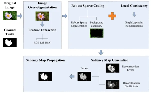
Fig. 2 illustrates the diagram of the proposed method, mainly consisting
185
of three parts: image over-segmentation and feature extraction, robust sparse
coding with local consistency, saliency map generation and propagation. In the
[image:9.612.152.454.270.456.2]following contents, we will elaborate each part.
Figure 2: Diagram of the proposed salient object detection.
3.2.1. Image over-segmentation and feature extraction
In our proposed method, the input image I is first over-segmented into N
190
super-pixels S = [s1, s2, . . . , sN] by using the simple linear iterative clustering
(SLIC) algorithm [33] due to its simplicity and efficiency. For each super-pixel
si, a feature vectorxi∈Rm of dimensionm= 9 is constructed, which includes
its red-, green-, and blue-components in RGB color space, its lightness- and two
color-opponent-components in the CIELab color space, and its hue-, saturation-,
195
and value-components in the HSV color spaces. On top of it, the feature vector
pixels contained in the current super-pixel. Finally, horizontally stacking the
feature vectors of all superpixels produces a feature matrixX ∈Rm×N for the input image, i.e.,X = [x1, x2, . . . , xN]∈Rm×N.
200
3.2.2. Background dictionary construction
Similar to other SR based salient object detection methods, the predefined
dictionary plays an important role in the proposed RSR based method.
Mo-tivated by its successful applications in the salient object detection methods
[12, 15, 16, 17, 27, 28], we also use the image boundary prior to construct a
205
background dictionary D = [d1, d2, . . . , dK] ∈ Rm×K in the RSR model. In
such a background dictionaryD,di∈Rmdenotes the feature vector of a
super-pixel near the image boundary, and K refers to the number of the dictionary
atoms. Here, we simply extract all the super-pixels that directly connect the
image border to construct the background dictionary.
210
3.2.3. Robust sparse coding with local consistency
Using the dictionary D ∈ Rm×K constructed in the previous sub-section, each super-pixel could be sparsely represented if directly applying the RSR
model in Eq. (1). However, this ignores the strong correlations among the
spa-tially local regions [17], and thus will be unavoidable for some isolated regions
in the detected result. In principle, the spatially adjacent super-pixels with
similar features should have similar saliency values [17]. Correspondingly, these
suppixels will have similar representation coefficients and reconstruction
er-rors when sparsely coded by using RSR with respect to the same background
dictionary. We achieve that by imposing two Laplacian regularizations on the
representation coefficients and reconstruction errors. The resulting salient
ob-ject detection model is formulated as follows.
min
Z,EkZk1+λ1kEk2,1+λ2tr(ZLZ T) +λ
3tr(ELET)
s.t. X =DZ+E
(2)
respective-ly. D is the predefined background dictionary. The Laplacian regularizations
tr(ZLZT) andtr(ELET) are defined as
tr(ZLZT) = 1 2
N
X
i,j
kzi−zjk 2
2ωij (3)
tr(ELET) =1 2
N
X
i,j
kei−ejk22ωij (4)
In Eq. (3) and Eq. (4),zi and ei denote the i-th columns of the matrices Z
andE, respectively. The weightωij implies the similarity between thei-th and
j-th super-pixels and will be discussed later in detail. Based on these weights,
an affinity matrixW ∈RN×N with its (i, j)-th entryWi,j=ωij and a diagonal
215
degree matrix C ∈ RN×N with its i-th diagonal element C
i,i = P j
Wi,j are
constructed. The Laplacian matrix L is thus defined as L =C−W. λ1, λ2,
andλ3 are three positive trade-off parameters.
The weightωij is computed by Eq. (5) in this paper.
ωij =
exp(−kpi−pjk22
2σ2
p )·exp(−
kxi−xjk2 2
2σ2
f
), if si andsj are spatially adjacent,
0, otherwise.
(5)
where pi, pj ∈ R2 denote the center positions of the super-pixels si and sj.
xi, xj ∈Rm are their feature vectors, respectively. σp andσf are two scalars,
220
and are experimentally set to√0.5 and 1, respectively.
In Eq. (5), the component, exp(−kpi−pjk22
2σ2
p ), denotes the spatial distance
between the two super-pixels si and sj, and the component, exp(−
kxi−xjk22
2σ2
f
),
indicates their feature similarity. Eq. (5) ensures that two super-pixels with
smaller spatial distance and more similar features are assigned to higher weight
225
values, thus preserving the local consistency among the spatially adjacent
super-pixels with similar features.
Fig. 3 illustrates the validity of the two Laplacian regularization terms.
Compared with those detection results obtained by the RSR model without
considering the local consistency (i.e., Fig. 3(b)), the performance is improved
230
Figure 3: Illustrations of the validity of the two Laplacian regularization terms. (a) Original
image; Saliency maps obtained by the RSR model (b) without considering the local
con-sistency; (c) imposing the Laplacian regularization only on the representation coefficients;
(d) imposing the Laplacian regularization only on the reconstruction errors; (e) imposing
t-wo Laplacian regularizations on the representation coefficients and reconstruction errors; (f)
Ground truth.
Fig. 3(c) and (d)). As well, compared with the detection results obtained
by imposing one Laplacian regularization term (i.e., Fig. 3(c) and (d)), the
performance is further improved by using two Laplacian regularization terms.
More specifically, the foreground salient object is more uniformly highlighted (as
235
shown in the first two rows in Fig. 3), and the background noise is also better
suppressed (as shown in the last two rows in Fig 3) by using two Laplacian
regularization terms than using one of the two Laplacian regularization terms.
The optimization algorithm is convex and can be solved by various methods.
In this paper, we jointly adopt the Alternating Direction Method of Multipliers
(ADMM) [34] and a modified Sparse Reconstruction by Separable
Approxima-tion (SpaRSA)-based method [35] to solve the optimizaApproxima-tion problem in Eq. (2).
This requires the minimization of the following augmented Lagrangian function:
L(Z, E, Y) =kZk1+λ1kEk2,1+λ2tr(ZLZT) +λ3tr(ELET)
+hY, X−DZ−Ei+µ2kX−DZ−Ek2F
(6)
con-straint in Eq. (2), andµis a penalty parameter. <·>denotes the Euclidean
240
inner product of two matrices. Clearly, this problem becomes unconstrained,
and can be minimized with respect toZ andE, respectively. Algorithm 1
sum-marizes the calculations of the optimization model. More details can be seen in
Appendix A.
Algorithm 1Solving the optimization problem in Eq. (6).
Input: Feature matrixX, parametersλ1,λ2,λ3, and Laplacian matrixL.
Output: Z andE
1: intialize: Z(0) =0, E(0) =0, Y(0) =0, µ(0) = 1,µ
max = 1010, ρ= 1.1,
t= 0,ε1= 10−3, andε2= 10−6.
2: repeat
3: FixE and updateZ using Eq. (A.4).
4: FixZ and updateE using Eq. (A.9).
5: Update the multiplierY: Y(t+1)=Y(t)+µ(t)(X−DZ(t)−E(t)).
6: Updateµ:
µ(t+1)=
min(ρµ(t), µmax), if µ(t)×max
Z(t+1)−Z(t) F,
E(t+1)−E(t) F
< ε1
µ(t), otherwise.
,
7: Updatet: t=t+ 1.
8: untilConvergence: X−DZ(t)−E(t)
F
kXk
F < ε2
3.2.4. Saliency Map Generation
245
In this part, we will explain how we compute the saliency measure for each
super-pixel as well as how we compute the saliency value for each pixel.
A. Saliency measure for each super-pixel.
Given a background dictionaryD, each column of the sparse errors matrixE
obtained by solving the model in Eq. (6) may contain the salient information of
250
each super-pixel that is distinct from the background. In addition, the
represen-tation coefficients may reflect the similarity between each test super-pixel and
each super-pixel consists of two sub-indexes in this paper. One is based on the
reconstruction errors while the other is based on the representation coefficients.
255
Generally, a super-pixel will be more salient if it has larger reconstruction
errors with respect to the background dictionary. Considering that, we define
the reconstruction errors based saliency measure SalE(si) for the i-th
super-pixelsi as
SalE(si) = 1−exp(−
ke∗ik22
2σ2 E
) (7)
wheree∗i denotes thei-th column vector of the optimal errors matrixE∗obtained by solving Eq. (6) and corresponds to the reconstruction errors of the
super-pixelsi. ke∗ik2represents thel2-norm of the vectore ∗
i and is defined aske∗ik2=
q P
j(e ∗ i(j))
2
. σE is a scalar parameter and is experimentally set to 4 here.
In addition to the reconstruction errors, the saliency value of each
super-260
pixel can also be determined by its representation coefficients to some extent.
For example, as shown in Fig. 4(a), a background super-pixel will be
sparse-ly coded by the predefined background dictionary. In contrast, as shown in
Fig. 4(b), a foreground super-pixel will be densely coded by the same
back-ground dictionary. In other words, the saliency value of each super-pixel can be
265
determined by the sparsity (also called coding length) of its representation
coef-ficients. As well, the foreground object in an image usually has higher contrast
than the background and thus has higher energy. Correspondingly, as shown in
Fig. 4, the representation coefficients for a foreground super-pixel have higher
magnitudes than those for a background super-pixel.
270
Based on the above two observations, we define the representation
coeffi-cients based saliency measureSalZ(si) for the i-th super-pixel as
SalZ(si) =kzi∗k0· 1−exp −
kzi∗k22
2σ2 Z
!!
(8)
wherez∗
i denotes thei-th column vector of the optimal representation matrixZ∗
obtained by solving Eq. (6) and corresponds to the representation coefficients
of the super-pixelsi. kz∗ik0represents thel0-norm of the vectorzi∗ and defined
Figure 4: Comparisons of representation coefficients of background and foreground
super-pixels. (a) Representation coefficients for a background super-pixel; (b) Representation
coef-ficients for a foreground super-pixel.
sparsity and the energy of the representation coefficients corresponding to the
275
super-pixelsi to some extent, respectively. Similarly,σZ is a scalar parameter
and is experimentally set to 4 in this paper.
The final saliency measureSal(si) for the super-pixel si is defined by
inte-grating the two saliency measuresSalE(si) andSalZ(si) as
Sal(si) =SalE(si)α.∗SalZ(si)1−α (9)
whereα∈(0,1) is a scalar to control the contributions of the two terms and is
set to 0.8 in the experiment par.
B. Saliency measure for each pixel.
280
According to the saliency measure defined by Eq. (9), an initial
super-pixel level saliency map Msp(si), i.e., Msp(si) = Sal(si), is obtained. After
that, a smooth saliency mapMsp0 (si) is obtained by performing the propagation
method [16] on the mapMsp(si). Finally, a pixel-level saliency mapMpixel(p)
is obtained by mapping the saliency mapM0
sp(si) to the full-resolution image,
i.e.,
Mpixel(p) =Msp0 (si), if p∈si (10)
Fig. 5 illustrates the saliency detection results obtained by different phases.
uniformly detect the whole salient object than those measures defined by Eq.
(7) or Eq. (8) independently. After the saliency map propagation, the salient
object is further uniformly highlighted. Meanwhile, the background is also well
285
[image:16.612.154.452.200.289.2]suppressed.
Figure 5: Saliency maps obtained by different saliency measures. (a) Original image; (b)
Saliency maps obtained by using the reconstruction errors; (c) Saliency maps obtained by
using the representation coefficients; (d) Saliency maps by fusing (b) and (c); (e) Saliency
maps after propagation; (f) Ground truth.
3.3. Computational complexity
Suppose the data matrixX and dictionaryD have sizesd×N andd×M,
respectively. Then the coefficients matrixZ has size M ×N. As discussed in
[18], the computational complexity of Algorithm 1 is mainly dependent on the
290
product of three matrices in Eq. (A.3) when the matrixZ is updated. Then the
computational complexity of the proposed method is thus O(rdM2N), where r is the number of iterations needed for convergence. It demonstrates that
the number of dictionary atomsM has a greater impact on the computational
complexity of the proposed method than other parameters. In the proposed
295
method,M is set to the number of boundary super-pixels (about 49), which is
far smaller than the total number of super-pixelsN (about 200). This makes
the computational cost of the proposed method acceptable.
4. Experiments and analysis
In this section, several sets of experiments are performed to verify the
supe-300
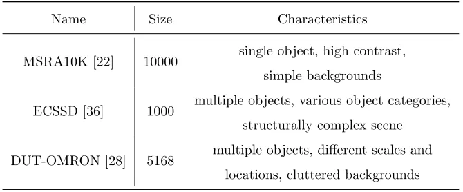
Table 1: Summary of the public datasets.
Name Size Characteristics
MSRA10K [22] 10000 single object, high contrast, simple backgrounds
ECSSD [36] 1000 multiple objects, various object categories, structurally complex scene
DUT-OMRON [28] 5168 multiple objects, different scales and locations, cluttered backgrounds
Table 2: Summary of the evaluation metrics.
Name Description
Precision-recall (PR) [2] Precision (P): |S∩G||S| , recall (R): |S∩G||G| F-measure [2] Fβ = (1 +β2)β2P∗RP+R,β
2= 0.3
precision, recall, and F-measure
with an adaptive threshold [20]
thre= W×H2 PW
i=1
PH
j=1S(i, j)
mean absolute error (MAE) [2] M AE= W1×HPW
i=1
PH
j=1|S(i, j)−G(i, j)|
4.1. Experimental setup
4.1.1. Datesets
In our experiments, we employ three public datesets, including MSRA10K
[22], ECSSD [36], and DUT-OMRON [28], to test the superiority of our proposed
305
method. The detailed descriptions for these datasets are presented in the Table
1.
4.1.2. Evaluation metrics
In the experiments, we adopt multiple evaluation metrics to verify the
supe-riority of our proposed method. Table 2 shows the summary of the evaluation
310
metrics. In the Table 2,S andGrepresent a saliency map and the
the mask. S(i, j) represents the saliency value of the (i, j)-th pixel inS. W and
H are the width and height of the image, respectively.
4.1.3. Parameters setting
[image:18.612.163.445.197.374.2]315
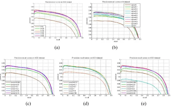
Figure 6: PR curves of the proposed method with different parameters values on the ASD
dataset. (a)N; (b)α; (c)λ1; (d)λ2; (e)λ3.
The parameters of our method involve the number of superpixels N, the
fusion weightαin Eq. (9), and the balance parameters λ1, λ2, and λ3 in Eq.
(2). The setting of these parameters is important to the performance of the
proposed method. We experimentally set the values of these parameters based
on the performance of the proposed method on the ASD dataset [20], which
320
has 1000 images. This dataset has similar characteristics with the MSRA10K
dataset due to the fact that they are both collected from the MSRA database
[37]. Each of them is set one by one, respectively, by fixing the others. More
specifically, in the experimental part, we test the impacts of the parametersN
(withα = 0.8, λ1 = 0.1, λ2 = 0.01, λ3 = 0.01), α (with N = 200, λ1 = 0.1,
325
λ2 = 0.01, λ3 = 0.01), λ1 (with N = 200,α= 0.8,λ2 = 0.01, λ3 = 0.01), λ2
(withN = 200,α= 0.8,λ1= 0.1,λ3= 0.01), andλ3 (withN = 200,α= 0.8,
λ1 = 0.1, λ2 = 0.01) on the proposed method, respectively. The PR curves of
From Fig. 6(a), it can be found that the performance increases withN, but
330
nearly unchanged whenN is greater than or equal to 200. So, we setN = 200.
The rest of parameters are set in a similar way. In summary, these parameters
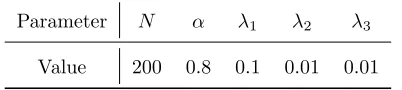
[image:19.612.205.406.221.266.2]are set to the values as in Table 3.
Table 3: Some parameters employed in our proposed method.
Parameter N α λ1 λ2 λ3
Value 200 0.8 0.1 0.01 0.01
4.1.4. Experiments
First, we employ the public dataset, MSRA10K [22] to illustrate the validity
335
of the robust sparse representation model and local consistency prior when
ap-plied to the detection of salient objects. Then, we employ three public datasets,
including MSRA10K [22], ECSSD [36], and DUT-OMRON [28], to test the
su-periority of our proposed method. Finally, we analyze some failure examples of
our proposed method.
340
4.2. Validity of RSR model and local consistency prior
In this part, we will employ the MSRA10K [22] dataset to illustrate the
validity of the RSR model and local consistency prior employed in our proposed
method. For that, we compare our proposed method (RSR-LC, for short) with
another three methods, including a RSR based (RSR-B, for short) and two
345
SR based (SR-S, SR-B, for short) methods mentioned in Fig. 1 in the earlier
Introduction part. The RSR-B method can be seen as a special case of our
proposed method withλ2 =λ3 = 0 in Eq. (3), without considering the local
consistency prior. In RSR-B and SR-B methods, a global background dictionary
obtained from the image boundary is employed. And in the SR-S method, a
350
local dictionary using the image patches surrounding each test image patch is
employed. Some detected results by these four methods can be seen in Fig. 1
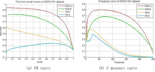
Fig. 7 provides the quantitative results of the four methods. It can be found
that the RSR-B method significantly outperforms the SR-S and SR-B methods
355
in terms of the PR and F-measure curves. This clearly shows the superiority
of the RSR model over the traditional SR model when applied to salient object
detection. Moreover, it can also be easily found that the local consistency prior
will further improve the performance by comparing the detected results of the
RSR-B method and the proposed method.
[image:20.612.167.439.257.383.2]360
Figure 7: Quantitative comparisons of the RSR-LC, RSR-B, SR-B, SR-S methods.
4.3. Superiority of the proposed method
In addition to the MSRA10K [22] dataset, we will employ another two public
benchmark datasets, i.e., ECSSD [36] and DUT-OMRON [28], to further test
the superiority of the proposed method. As well, we compare the proposed
method with another 9 state-of-the-art ones, including SR-LC [17], BFS [38],
365
HDCT [24], PCA [39], TD [40], GC [41], GS [15], SF [42], SS [43].
4.3.1. Visual comparison
Fig. 8 illustrates some detected results obtained by these methods. As shown
in Fig. 8, most of the methods mentioned in this paper could achieve satisfactory
results for all of the three datasets. But by a careful comparison, we find that
370
GC, HDCT, BFS and RSR-LC could obtain higher performance in foreground
detection and background suppression than the other methods in most cases.
third row in Fig. 8(a) and the second row in Fig. 8(b)), the proposed method
RSR-LC could still detect the whole objects. Similar results could also be
375
obtained by the proposed RSR-LC for those images with complex backgrounds
(e.g., the last row in Fig. 8(c)). For these images, most of the
state-of-the-art methods could not obtain a satisfactory result. In addition, we also find
that the proposed method RSR-LC significantly outperforms SR-LC for these
images. This further demonstrates the superiority of the RSR model over the
380
[image:21.612.153.457.261.606.2]traditional SR model.
Figure 8: Visual comparisons on different methods. (a) Results on the MSRA10K dataset;
4.3.2. Quantitative comparison
Fig. 9 provides the quantitative results of different methods, complying with
those subjective results mentioned in Fig. 8.
For MSRA10K dataset, our proposed method is competitive with
HDC-385
T and better than the other state-of-the-art methods in terms of PR and
F-measure curves. Given an appropriate threshold to segment the saliency map,
our proposed method will obtain the highest F-measure value among the
meth-ods mentioned here. Furthermore, our proposed method obtains a good MAE
value.
[image:22.612.164.443.293.565.2]390
Figure 9: Quantitative comparisons on different methods. From left to right: Results on
MSRA10K, ECSSD, and DUT-OMRON datasets, respectively. From top to bottom: PR
curves, F-measure curves, precision, recall, and F-measure bars with an adaptive threshold,
and MAE bars, respectively.
F-measure performance among the methods. That is to say, compared with the
state-of-the-arts, our proposed method is more effective in salient object
detec-tion for those images where multiple salient objects exist and belong to various
categories. Seen from the F-measure bars with an adaptive threshold, our
pro-395
posed method also obtains the highest F-measure value among the methods.
And our proposed method achieves the least MAE value.
For DUT-OMRON dataset, HDCT and our proposed method perform
com-petitively and are both better than the other state-of-the-art methods in terms
of the PR and F-measure curves. That is to say, our proposed method could
400
still achieve satisfactory results for images with more complex background
struc-tures. Given an appropriate threshold, our proposed method can obtain the
sec-ond best F-measure value among the methods. Moreover, our proposed method
achieves the best performance in terms of the metric of MAE.
4.3.3. Computational complexity comparison
405
To demonstrate the computational efficiency of our method, we list the
av-erage computational time of some state-of-the-art methods1 and our proposed method on the ASD dataset [20]. These methods are all run in Matlab 2013
on a personal computer with an Intel(R) Core(TM) i7-4790 3.60 GHz CPU. As
shown in Table 4, our proposed method (RSR-LC) is slightly slower than SR-LC
410
but much faster than PCA and BFS.
Table 4: Average running time of some methods (seconds per image).
Methods Ours SS PCA BFS SR-LC
Time (s) 1.7649 0.0219 2.4589 6.4427 1.2793
1Here we just list those compared methods whose Matlab codes are provided in their
4.4. Failure cases
In the proposed method, those super-pixels near the image boundary are
selected to construct the background dictionary based on the background prior
[15]. In most cases, this may work well. However, in some images, salient objects
415
appear near the image boundary, and thus some foreground regions will be
con-tained in the background dictionary. As a result, these foreground regions will
be mistakenly marked as background regions for these images. In addition, if
the background regions far from the image boundary and those near the image
boundary have obviously distinctive characteristics, some background regions
420
will also be mistakenly marked as foregrounds. Some failure cases are
illustrat-ed in Fig. 10. Exploiting more efficient background dictionary construction
[image:24.612.157.453.347.472.2]methods will overcome this problem and we leave this as the future work.
Figure 10: Failure cases. (a) Original images; (b) Saliency maps obtained by the proposed
method; (c) Ground truth.
5. Conclusion
In this paper, we have presented a new salient object detection method
425
that incorporates a local consistency prior into the robust sparse representation
(RSR) model. By virtue of RSR, salient objects can be seen as strong but sparse
“outliers” within an image, which allows to reformulate the salient object
detec-tion problem as a sparsity pursuit one. Given the same background dicdetec-tionary,
the RSR based method can better suppress the background noise than those
traditional SR based ones. Moreover, owing to the local consistency prior, the
whole salient object could be more uniformly highlighted. Experimental results
demonstrate that the proposed method significantly outperforms the traditional
SR based methods and is competitive with some current state-of-the-art
meth-ods, especially for those images with complex structures.
435
Acknowledgement
This work is supported by the National Natural Science Foundation of China
under Grant No. 61104212, by Natural Science Basic Research Plan in Shaanxi
Province of China (Program No. 2016JM6008), and by the Fundamental
Re-search Funds for the Central Universities under Grant No. NSIY211416.
440
Appendix
Appendix A.
In this appendix, the update scheme required for solving Eq. (6) in the text
is described in detail.
(1) Update Z:
445
Z= arg min
Z kZk1+λ2tr(ZLZ
T) +hY, X−DZ−Ei+µ
2kX−DZ−Ek
2 F
= arg min
Z kZk1+λ2tr(ZLZ T
) +µ 2
X−DZ−E+1 µY 2 F
= arg min
Z kZk1+f(Z)
(A.1)
wheref(Z) =λ2tr(ZLZT) + µ2
X−DZ−E+
1 µY 2 F
. This sub-optimization
problem can be solved by using the modified SpaRSA-based method [35] in an
iterated way, i.e.,
Z(t+1)= arg min
Z
1
η(t)Z
kZk1+1 2
Z−(Z(t)− 1
ηZ(t)
∇Zf(Z(t)))
whereη(t)Z = 1.022λ2kLk2F+µ(t)
DTD
2 F
[44, 45]. ∇Zf(Z(t)) is the partial
differential off(Z) with respect toZ in thet-th iteration, and is computed by:
∇Zf(Z(t)) = 2λ2Z(t)L−µDT(X−DZ(t)−E(t)+
1 µ(t)Y
(t)) (A.3)
Thus, the sub-optimization problem in Eq. (A.2) has the following closed-form
solution [34]:
Z(t+1)=S 1
η(Zt)
Z(t)− 1
ηZ(t)
∇Zf(Z(t))
!
(A.4)
where the threshold functionSτ(x) is defined as
Sτ(x) =
x−τ, if x > τ
x+τ, if x <−τ
0, otherwise
(A.5)
(2) Update E:
E= arg min
E λ1kEk2,1+λ3tr(ELE
T) +hY, X−DZ−Ei+µ
2kX−DZ−Ek
2 F
= arg min
E λ1kEk2,1+λ3tr(ELE T) +µ
2
X−DZ−E+ 1 µY 2 F
= arg min
E λ1kEk2,1+f(E)
(A.6)
where f(E) = λ3tr(ELET) + µ2
X−DZ−E+
1 µY 2
F. Similarly, this
sub-optimization problem can also be solved by using the modified SpaRSA-based
method [33] in an iterated way, i.e.,
E(t+1)= arg min
E
λ1
η(t)E kEk2,1+ 1 2
E− E(t)− 1
η(t+1)E ∇Ef
E(t) ! 2 F (A.7)
where ηE(t) = 1.022λ3kLk 2 F+µ
(t) [44, 45]. ∇
Ef(E(t)) is the partial
differ-ential of f(E) with respect to E in the t-th iteration, and is computed by:
∇Ef(E(t)) = 2λ3E(t)L−µ(X−DZ(t)−E(t)+
1 µY
The sub-optimization problem in Eq. (A.7) has the following closed-form
solu-tion [34]
E(t+1)(:, i) =
kG(:,i)k2− λ1
η(Et)
!
kG(:,i)k2 G(:, i), if kG(:, i)k2≥ λ1
η(Et)
0, otherwise
(A.9)
whereG=E(t)− 1
η(Et)∇Ef E (t)
. E(:, i) andG(:, i) denote thei-th columns of
the matricesE andG, respectively.
References
[1] P. Jiang, H. Ling, J. Yu, J. Peng, Salient region detection by UFO:
u-450
niqueness, focusness and objectness, in: IEEE International Conference on
Computer Vision, 2013, pp. 1976–1983.
[2] A. Borji, M. M. Cheng, H. Jiang, J. Li, Salient object detection: A
bench-mark, IEEE Transactions on Image Processing 24 (12) (2015) 5706–5722.
[3] J. Han, K. N. Ngan, M. Li, H. J. Zhang, Unsupervised extraction of visual
455
attention objects in color images, IEEE Transactions on Circuits & Systems
for Video Technology 16 (1) (2006) 141–145.
[4] P. Peng, L. Shao, J. Han, J. Han, Saliency-aware image-to-class distances
for image classification, Neurocomputing 166 (C) (2015) 337–345.
[5] G. Liu, Z. Lin, S. Yan, J. Sun, Y. Yu, Y. Ma, Robust recovery of subspace
460
structures by low-rank representation, IEEE Transactions on Pattern
Anal-ysis & Machine Intelligence 35 (1) (2013) 171–184.
[6] D. Gao, S. Han, N. Vasconcelos, Discriminant saliency, the detection of
sus-picious coincidences, and applications to visual recognition, IEEE
Transac-tions on Pattern Analysis & Machine Intelligence 31 (6) (2009) 989–1005.
465
[7] P. Wang, J. Wang, G. Zeng, J. Feng, Salient object detection for searched
web images via global saliency, in: IEEE Conference on Computer Vision
[8] J. Han, E. J. Pauwels, P. De Zeeuw, Fast saliency-aware multi-modality
image fusion, Neurocomputing 111 (6) (2013) 70–80.
470
[9] Y. Li, Y. Zhou, L. Xu, X. Yang, Incremental sparse saliency detection, in:
International Conference on Image Processing, 2009, pp. 3093–3096.
[10] B. Han, H. Zhu, Y. Ding, Bottom-up saliency based on weighted sparse
coding residual, in: International Conference on Multimedea, 2011, pp.
1117–1120.
475
[11] J. Yan, M. Zhu, H. Liu, Y. Liu, Visual saliency detection via sparsity
pursuit, IEEE Signal Processing Letters 17 (8) (2010) 739–742.
[12] N. Li, B. Sun, J. Yu, A weighted sparse coding framework for saliency
detec-tion, in: IEEE Conference on Computer Vision and Pattern Recognidetec-tion,
2015, pp. 5216–5223.
480
[13] J. Wright, A. Y. Yang, A. Ganesh, S. S. Sastry, Y. Ma, Robust face
recog-nition via sparse representation, IEEE Transactions on Pattern Analysis &
Machine Intelligence 31 (2) (2009) 210–227.
[14] C. Li, Y. Ma, X. Mei, C. Liu, Hyperspectral image classification with robust
sparse representation, IEEE Geoscience & Remote Sensing Letters 13 (5)
485
(2016) 641–645.
[15] Y. Wei, F. Wen, W. Zhu, J. Sun, Geodesic saliency using background priors,
in: European Conference on Computer Vision, 2012, pp. 29–42.
[16] H. Lu, X. Li, L. Zhang, R. Xiang, Dense and sparse reconstruction error
based saliency descriptor, IEEE Transactions on Image Processing 25 (4)
490
(2016) 1–1.
[17] L. Huo, S. Yang, L. Jiao, S. Wang, S. Wang, Local graph regularized sparse
reconstruction for salient object detection, Neurocomputing 194 (C) (2016)
[18] Q. Zhang, M. D. Levine, Robust multi-focus image fusion using multi-task
495
sparse representation and spatial context, IEEE Transactions on Image
Processing 25 (5) (2016) 2045–2058.
[19] L. Itti, C. Koch, E. Niebur, A model of saliency-based visual attention for
rapid scene analysis, IEEE Transactions on Pattern Analysis & Machine
Intelligence 20 (11) (1998) 1254–1259.
500
[20] R. Achanta, S. Hemami, F. Estrada, S. Susstrunk, Frequency-tuned salient
region detection, in: IEEE International Conference on Computer Vision
and Pattern Recognition, 2009, pp. 1597–1604.
[21] R. Achanta, S. Ssstrunk, Saliency detection using maximum symmetric
surround, in: IEEE International Conference on Image Processing, 2010,
505
pp. 2653–2656.
[22] M. M. Cheng, N. J. Mitra, X. Huang, P. H. S. Torr, S. M. Hu,
Glob-al contrast based sGlob-alient region detection, IEEE Transactions on Pattern
Analysis & Machine Intelligence 37 (3) (2015) 569–582.
[23] J. Ren, X. Gong, L. Yu, W. Zhou, M. Y. Yang, Exploiting global priors
510
for rgb-d saliency detection, in: IEEE Conference on Computer Vision and
Pattern Recognition Workshops, 2015, pp. 25–32.
[24] J. Kim, D. Han, Y. W. Tai, J. Kim, Salient region detection via
high-dimensional color transform, in: IEEE Conference on Computer Vision
and Pattern Recognition, 2014, pp. 883–890.
515
[25] N. Tong, H. Lu, Y. Zhang, X. Ruan, Salient object detection via global and
local cues, Pattern Recognition 48 (10) (2015) 3258–3267.
[26] Q. Fan, C. Qi, Saliency detection based on global and local short-term
sparse representation, Neurocomputing 175 (2016) 81–89.
[27] W. Zhu, S. Liang, Y. Wei, J. Sun, Saliency optimization from robust
back-520
ground detection, in: IEEE Conference on Computer Vision and Pattern
[28] C. Yang, L. Zhang, H. Lu, R. Xiang, Saliency detection via graph-based
manifold ranking, in: IEEE Conference on Computer Vision and Pattern
Recognition, 2013, pp. 3166–3173.
525
[29] D. A. Klein, S. Frintrop, Center-surround divergence of feature statistics for
salient object detection, in: IEEE Conference on Computer Vision, 2011,
pp. 2214–2219.
[30] L. Wang, H. Lu, X. Ruan, M. H. Yang, Deep networks for saliency detection
via local estimation and global search, in: IEEE Conference on Computer
530
Vision and Pattern Recognition, 2015, pp. 3183–3192.
[31] W. Wang, J. Shen, L. Shao, Consistent video saliency using local
gradi-ent flow optimization and global refinemgradi-ent, IEEE Transactions on Image
Processing 24 (11) (2015) 4185–96.
[32] Y. Han, Y. Yang, Y. Yan, Z. Ma, N. Sebe, X. Zhou, Semisupervised feature
535
selection via spline regression for video semantic recognition, IEEE
Trans-actions on Neural Networks & Learning Systems 26 (2) (2015) 252–264.
[33] R. Achanta, A. Shaji, K. Smith, A. Lucchi, P. Fua, S. SuSstrunk, SLIC
superpixels compared to state-of-the-art superpixel methods, IEEE
Trans-actions on Pattern Analysis & Machine Intelligence 34 (11) (2012) 2274–82.
540
[34] S. Boyd, N. Parikh, E. Chu, B. Peleato, J. Eckstein, Distributed
optimiza-tion and statistical learning via the alternating direcoptimiza-tion method of
multi-pliers, Foundations & Trends in Machine Learning 3 (1) (2010) 1–122.
[35] S. J. Wright, R. D. Nowak, M. A. T. Figueiredo, Sparse reconstruction by
separable approximation, IEEE Transactions on Signal Processing 57 (7)
545
(2009) 3373–3376.
[36] J. Shi, Q. Yan, L. Xu, J. Jia, Hierarchical image saliency detection on
extended cssd, IEEE Transactions on Pattern Analysis & Machine
[37] T. Liu, J. Sun, N. N. Zheng, X. Tang, Learning to detect a salient object,
550
in: IEEE Conference on Computer Vision and Pattern Recognition, 2007,
pp. 1–8.
[38] J. Wang, H. Lu, X. Li, N. Tong, W. Liu, Saliency detection via background
and foreground seed selection, Neurocomputing 152 (C) (2015) 359–368.
[39] M. Ran, A. Tal, L. Zelnikmanor, What makes a patch distinct?, in: IEEE
555
Conference on Computer Vision and Pattern Recognition, 2013, pp. 1139–
1146.
[40] C. Scharfenberger, A. Wong, K. Fergani, J. S. Zelek, Statistical textural
distinctiveness for salient region detection in natural images, in: IEEE
Conference on Computer Vision and Pattern Recognition, 2013, pp. 979–
560
986.
[41] M. M. Cheng, J. Warrell, W. Y. Lin, S. Zheng, Efficient salient region
detection with soft image abstraction, in: IEEE Conference on Computer
Vision, 2013, pp. 1529–1536.
[42] P. Krahenbuhl, Saliency filters: Contrast based filtering for salient region
565
detection, in: IEEE Conference on Computer Vision and Pattern
Recogni-tion, 2012, pp. 733–740.
[43] X. Hou, J. Harel, C. Koch, Image signature: Highlighting sparse salient
regions, IEEE Transactions on Pattern Analysis & Machine Intelligence
34 (1) (2012) 194–201.
570
[44] M. Yin, J. Gao, Z. Lin, Laplacian regularized low-rank representation and
its applications, IEEE Transactions on Pattern Analysis & Machine
Intel-ligence 38 (3) (2016) 504–517.
[45] D. Tao, J. Cheng, M. Song, X. Lin, Manifold ranking-based matrix
factor-ization for saliency detection, IEEE Transactions on Neural Networks &
575
![Figure 1: Typical challenging examples for SR based salient object detection methods. (a)Original images; (b) SR based method with surrounding patches as the dictionary [10]; (c)SR based method with background templates near the image boundary as the backgrounddictionary; (d) Proposed RSR method with the background dictionary but without the localconsistency prior; (e) Proposed RSR method with the background dictionary as well as thelocal consistency prior; (f) Ground truth.](https://thumb-us.123doks.com/thumbv2/123dok_us/9337344.435764/3.612.156.452.215.436/challenging-surrounding-dictionary-backgrounddictionary-background-dictionary-localconsistency-consistency.webp)