Tidal range energy resource and optimization past perspectives and future challenges

(1)

Tidal range energy resource and optimization – past

1

perspectives and future challenges

2

Simon P. Neilla,∗, Athanasios Angeloudisb, Peter E. Robinsa, Ian

3

Walkingtonc_{, Sophie L. Ward}a_{, Ian Masters}d_{, Matt J. Lewis}a_{, Marco} 4

Pianoa_{, Alexandros Avdis}b_{, Matthew D. Piggott}b_{, George Aggidis}f_{, Paul} 5

Evansg, Thomas A. A. Adcockh, Audrius ˇZidonisf, Reza Ahmadiane, Roger

6

Falconere 7

a_{School of Ocean Sciences, Bangor University, Marine Centre Wales, Menai Bridge, UK}

8

b_{Department of Earth Science and Engineering, Imperial College London, UK}

9

c_{School of Natural Sciences and Psychology, Department of Geography, Liverpool John}

10

Moores University, Liverpool, UK

11

d_{College of Engineering, Swansea University, Bay Campus, Swansea, UK}

12

e_{School of Engineering, Cardiff University, The Parade, Cardiff, UK}

13

f_{Engineering Department, Lancaster University, Lancaster, UK}

14

g_{Wallingford HydroSolutions, Castle Court, 6 Cathedral Road, Cardiff, UK}

15

h_{Department of Engineering Science, University of Oxford, Oxford, UK}

16

Abstract

17

Tidal energy is one of the most predictable forms of renewable energy.

Al-18

though there has been much commercial and R&D progress in tidal stream

19

energy, tidal range is a more mature technology, with tidal range power plants

20

having a history that extends back over 50 years. With the 2017 publication

21

of the “Hendry Review” that examined the feasibility of tidal lagoon power

22

plants in the UK, it is timely to review tidal range power plants. Here, we

23

explain the main principles of tidal range power plants, and review two main

24

research areas: the present and future tidal range resource, and the

opti-25

mization of tidal range power plants. We also discuss how variability in the

26

electricity generated from tidal range power plants could be partially offset

27

by the development of multiple power plants (e.g. lagoons) that are

comple-28

∗

(2)

mentary in phase, and by the provision of energy storage. Finally, we discuss

29

the implications of the Hendry Review, and what this means for the future

30

of tidal range power plants in the UK and internationally.

31

Keywords: Tidal lagoon, Tidal barrage, Resource assessment,

32

Optimization, Hendry Review, Swansea Bay

33

Contents

34

1 Introduction 3

35

2 A brief history of tidal range schemes 7

36

2.1 Commercial progress . . . 7

37

2.1.1 Current schemes . . . 7

38

2.1.2 Proposed schemes . . . 9

39

2.2 Engineering aspects of tidal range power plants . . . 10

40

3 Numerical simulations of tidal range power plants 12

41

3.1 0D modelling . . . 12

42

3.2 1D modelling . . . 14

43

3.3 2D and 3D models . . . 15

44

3.4 Observations and validation . . . 19

45

4 Tidal range resource 20

46

4.1 Theoretical global resource . . . 20

47

4.2 Theoretical resource of the European shelf seas . . . 22

48

4.3 Non-astronomical influences on the resource . . . 26

49

4.4 Long timescale changes in the tidal range resource . . . 27

(3)

4.5 Socio-techno-economic constraints on the theoretical resource . 28

51

5 Optimization 31

52

5.1 Energy optimization . . . 31

53

5.2 Economic optimization . . . 33

54

5.3 Implications of regional hydrodynamics for individual lagoon

55

resource . . . 34

56

5.4 Multiple lagoon resource optimization . . . 35

57

6 Challenges and opportunities 37

58

6.1 Variability and storage . . . 37

59

6.2 Additional socio-economic benefits through multiple use of space 39

60

6.3 Implications of the Hendry Review . . . 40

61

7 Conclusions 42

62

1. Introduction

63

Much of the energy on Earth that is available for electricity generation,

64

particularly the formation of hydrocarbons, originates from the Sun. This

65

also includes renewable sources of electricity generation such as solar, wind

66

& wave energy, and hydropower (since weather patterns are driven, to a

67

significant extent, by the energy input from the Sun). However, one key

68

exception is the potential for electricity generation from the tides – a result

69

of the tide generating forces that arise predominantly from the coupled

(4)

Moon system1_{. The potential for converting the energy of tides into other} 71

useful forms of energy has long been recognised; for example tide mills were

72

in operation in the middle ages, and may even have been in use as far back as

73

Roman times [1]. The potential for using tidal range to generate electricity

74

was originally proposed for the Severn Estuary in Victorian times [2], and

75

La Rance (Brittany) tidal barrage – the world’s first tidal power plant – has

76

been generating electricity since 1966 [3]. However, only very recently has the

77

strategic case for tidal lagoon power plants been comprehensively assessed,

78

with the publication of the “Hendry Review” in January 2017 [4].

79

Tidal range power plants are defined as dams, constructed where the

80

tidal range is sufficient to economically site turbines to generate electricity.

81

The plant operation is based on the principle of creating an artificial tidal

82

phase difference by impounding water, and then allowing it to flow through

83

turbines. The instantaneous potential power (P) generated is proportional

84

to the product of the impounded wetted surface area (A) and the square of

85

the water level difference (H) between the upstream and downstream sides

86

of the impoundment:

87

P ∝AH2 (1)

A tidal range power plant consists of four main components [5, 6]:

88

• Embankments form the main artificial outline of the impoundment, and

89

are designed to have a minimal length while maximizing the enclosed

90

plan surface area. A key factor in designing the embankment is to

91

1_{The Sun also has an important role in tides, but its contribution is around half that}

(5)

minimise disturbance to the natural tidal flow.

92

• Turbines are located in water passages across the embankment, and

93

convert the potential energy created by the head difference into

rota-94

tional energy, and subsequently into electricity via generators.

95

• Openings are fitted with control gates, or sluice gates, to transfer flows

96

at a particular time, and with minimal obstruction.

97

• Locks are incorporated along the structure to allow vessels to safely

98

pass the impoundment.

99

Tidal range power plants can be either coastally attached (such as a

bar-100

rage) or located entirely offshore (such as a lagoon). The primary difference

101

between the two refers to their impoundment perimeter. There are also

102

coastally-attached lagoons, where the majority of the perimeter is artificial,

103

potentially enabling smaller developments with more limited environmental

104

impacts than barrages – the latter generally spanning the entire width of an

105

estuary.

106

Following construction, the manner and how much of the potential energy

107

is extracted from the tides largely depends on the regulation of the turbines

108

and sluice gates [7]. They can be designed to generate power one-way, i.e.

109

ebb-only or flood-only, or bi-directionally. In one-way ebb generation, the

110

rising tide enters the enclosed basin through sluice gates and idling turbines.

111

Once the maximum level in the lagoon is achieved, these gates are closed,

112

until a sufficient head (hmax) develops on the falling tide. Power is

subse-113

quently generated until a predetermined minimum head difference (hmin),

114

when turbines are no longer operating efficiently. For flood generation the

(6)

whole process is reversed to generate power during the rising tide. In two-way

116

power generation, energy is extracted on both the flood and ebb phases of the

117

tidal cycle, with sluicing occurring around the times of high and low water

118

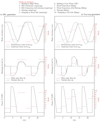
[8, 9]. A schematic representation of ebb and two-way generation modes of

119

operation is shown in Fig. 1, highlighting the main trigger points during the

120

tidal cycle that dictate power generation. Nonetheless, there are other

pos-121

sible variations of these regimes (e.g. Section 5.1). For example, ebb/flood

122

generation can often be supplemented with pumping water through the

tur-123

bines to further increase the water head difference values, as considered in

124

studies by Aggidis and Benzon [10] and Yates et al. [11].

125

In this article, we provide a review of tidal range power plants, with a

fo-126

cus on resource and optimization. The following section provides an overview

127

of the history of tidal range schemes from pre-industrialization to present day,

128

including future proposed schemes. Section 3 compares the various modelling

129

approaches used to simulate tidal lagoon or barrage operation (e.g. 0D versus

130

2D models), and Section 4 examines the global tidal range resource, with a

131

particular focus on the northwest European continental shelf, and constraints

132

on the development of this resource. Section 5 examines ways in which tidal

133

range schemes can be optimised, e.g. flood or ebb generation, pumping, and

134

the benefits of concurrently developing multiple tidal range schemes. Finally,

135

in Section 6, we discuss future challenges and opportunities facing tidal range

136

power plants, including variability and storage, and the implications of the

137

Hendry Review.

(7)

2. A brief history of tidal range schemes

139

Tidal range technologies have a long history, especially when compared

140

with less mature ocean energy technologies such as tidal stream and wave

141

energy. Energy has been extracted from the tides for centuries. There is

142

evidence of a tide mill in Strangford Lough, Northern Ireland, which has been

143

dated to the early 6th Century [1], where an 8 m wide dam enclosed a 6500 m2 144

area of sea water. Such early tidal power plants worked much as modern tidal

145

range projects, but used only naturally-occurring tidal basins to impound

146

volumes of water, which would then be routed through a paddlewheel or

147

waterwheel during the ebb. The extracted energy was, of course, not used to

148

generate electricity, but to provide mechanical motion, for example to mill

149

grain.

150

2.1. Commercial progress 151

Locations around the world that are suitable for tidal range exploitation

152

are relatively limited, given a number of physical constraints, including tidal

153

range, grid connectivity, geomorphology, seabed conditions, and available

154

area for an impoundment. There are five tidal range power plants currently

155

in operation around the world, and a number of areas that have either been

156

identified for development, or which exhibit suitable characteristics to merit

157

consideration.

158

2.1.1. Current schemes 159

La Rance tidal barrage in Brittany was the world’s first fully operational

160

tidal power station [3, 12, 13]. The project, which comprises a 720 m long

161

(8)

over a six-year period, and was fully operational in 1966 (Table 1). The

163

barrage houses 24 Kaplan bulb turbines, which provide a combined rated

164

power output of 240 MW and an annual energy output of 480 GWh [15].

165

Since its inception, there have not been any major structural issues, and very

166

little downtime, although there have been significant environmental impacts

167

[16].

168

The Kislaya Guba tidal power plant in Russia was constructed in 1968

169

as a trial project by the government, with an initial installed capacity of 400

170

kW [14]. It is situated near Murmansk, a fjord on the Kola Peninsula [13].

171

The installed capacity of this power plant has grown to 1.7 MW, which is

172

relatively low compared with other worldwide schemes, making it the smallest

173

tidal range power plant in operation [17]. However, the success of this scheme

174

has motivated the government to explore other sites, including Mezan Bay in

175

the White Sea and Tugar Bay, with potential installed capacities of 15 GW

176

and 6.8 GW respectively [17]. The former of the two figures is particularly

177

impressive, since this would be the second largest power plant in the world,

178

the largest being the 22.5 GW Three Gorges Dam in China [18].

179

The Annapolis Royal Generating Station was constructed in 1984, and

180

is located on the Annapolis River, Nova Scotia, Canada. It harnesses the

181

head difference created in the Annapolis Basin, a sub-basin of the Bay of

182

Fundy, which has a spring tidal range of 16 m [19]. This scheme consists

183

of a single Straflo turbine, and produces a peak power output of 20 MW on

184

the ebb tide only [13]. As well as generating electricity, this power plant is

185

also used for flood defence and serves as an important transport link – the

186

latter being a particularly advantageous and unique feature of barrages, for

(9)

example compared to a tidal lagoon.

188

The Jiangxia tidal range power plant was opened in 1985, and is located in

189

Jiangxia Port, Wenling, China, an area that is characterised by tidal ranges

190

of up to 8.4 m [13]. The power plant operates bi-directionally, and houses six

191

bulb turbines, the last of which was installed in 2007, providing an installed

192

capacity of 3.9 MW.

193

The largest (by installed capacity) tidal range scheme currently in

exis-194

tence is Lake Sihwa, which is situated in the mid-eastern region of the Korean

195

Peninsula in the Kyeonggi Bay, South Korea. The power plant stemmed from

196

a disused dam constructed in 1994 to hold irrigation water for agricultural

197

land; however, industrial developments in its vicinity caused pollution issues

198

[20]. To help tackle the pollution problems, the dam was subsequently

con-199

verted to a flood-operating tidal power plant [13]. The power plant

incorpo-200

rates 10 bulb turbines, with an installed capacity of 254 MW. The success of

201

this scheme has motivated the Korean government to explore other potential

202

sites around the country, including Gerolim and Incheon [13].

203

2.1.2. Proposed schemes 204

There are a number of factors that preclude development in certain areas,

205

even if first-order theoretical appraisals of the resource suggest that there is

206

commercial potential. Apart from physical constraints, cost and

environmen-207

tal impacts are other major barriers to development. Environmental issues,

208

particularly for larger scale schemes, have prevented numerous developments

209

from being approved [13]. Without constructing a scheme, its true

environ-210

mental impact is difficult to quantify, and so governments are hesitant to

211

proceed with development at such scale. Table 2 summarises sites around

(10)

the world that have the potential for tidal range exploitation.

213

A relatively recent tidal range concept that addresses some of these

envi-214

ronmental concerns is the tidal lagoon. These tidal range power plants differ

215

from the more conventional barrage schemes, as they impound a smaller body

216

of water and are therefore less intrusive. One such scheme is the proposed

217

Swansea Bay Lagoon, located in the Bristol Channel, UK, an area that is

218

characterized by tidal ranges that exceed 10 m [21].

219

Although no tidal lagoons currently exist, the Swansea Bay Lagoon is

220

the closest scheme to commercial viability. The UK Government have

re-221

cently completed an independent review which considered the feasibility of

222

the power plant in terms of cost effectiveness, supply chain opportunities,

223

possible structures to finance this project, and scales of design [22]. Despite

224

the positive outcome of the “Hendry Review” [4], a marine licence is still

re-225

quired from Natural Resources Wales (NRW)2, and an agreement on the CfD

226

(Contracts for Difference) price, before the project can proceed to

construc-227

tion. There are a number of other areas in the UK that have been identified

228

for development, as summarized in Table 2. However, it is likely that these

229

will only be approved on the condition that the Swansea Bay “Pathfinder

230

Project” proceeds and is successful.

231

2.2. Engineering aspects of tidal range power plants 232

Bulb turbines are used for power takeoff in almost all current tidal range

233

schemes [13]. These are the same, or very similar, to the turbines that are

234

used for low head hydropower applications. When low head hydro was

con-235

(11)

sidered as an energy solution for the UK in 1927, the investigating team (the

236

Severn Barrage Committee) found the Kaplan turbine to be the most

effi-237

cient for low head applications [23]. In the following years, as more research

238

has been conducted in the field of turbines, the bulb turbine, a configuration

239

of a Kaplan turbine, has become the turbine of choice for low head hydro or

240

tidal range schemes. Furthermore, triple regulation (adjustable guide vanes,

241

blade pitch angle and variable speed) of turbines has become feasible in

re-242

cent years [4, 13, 21], which will accommodate the constant varying head

243

conditions that are inevitable in tidal range applications.

244

Tidal range schemes will likely utilise this relatively mature turbine

tech-245

nology, with specific adaptations to better suit tidal environments. It is most

246

certain that the largest share of the cost is in the civil engineering work [4].

247

A potential reduction of the civil costs is proposed, which is the usage of

248

caissons. This would enable the construction of the turbine housing

struc-249

ture on land, as opposed to using cofferdams. It has to be taken into account

250

that in tidal range applications a longer water passage is required, as the

251

bulb turbines may work in two-way generation, as opposed to classical

one-252

way generation [7, 24]. Therefore, a draft tube is required on both sides of

253

the turbine. Recent suggestions for impoundment designs include the use of

254

geotubes and sand [6, 13]. These impoundments would also act as

break-255

water and sea defence structures, helping protect neighbouring regions from

256

flooding [e.g. 25].

(12)

3. Numerical simulations of tidal range power plants

258

The assessment of tidal range schemes relies on the development of

nu-259

merical tools that can simulate their operation over time. These span from

260

simplified theoretical and zero-dimensional (0D) models [8, 10, 26, 27] to more

261

sophisticated depth-averaged (2D) and hydro-environmental tools [9, 20, 24,

262

28, 29, 30, 31, 32, 33, 34, 35, 36, 37] that often require High Performance

263

Computing (HPC) capabilities for practical application.

264

3.1. 0D modelling 265

Given (a) known tidal conditions, (b) plant operation sequence, and (c)

266

appropriate formulae that represent the performance of constituent hydraulic

267

structures, it is feasible to simulate the overall performance of a tidal range

268

scheme, and provide an informed resource assessment [24]. The operation can

269

be modelled using a water level time series as input, governed by the transient

270

downstream water elevations at the site location (Fig. 1). This is known as

271

0D modelling, and has been deemed sufficient under certain conditions, e.g.

272

for smaller lagoons and barrages, as explored in the literature [28, 34, 35, 38].

273

A multitude of 0D models have been reported for the estimation of tidal

274

power plant electricity outputs [e.g. 27, 34, 39]. However, one commonly used

275

technique is the backward-difference numerical model, developed according

276

to the continuity equation. Given the downstream ηdn,i and upstream ηup,i

277

water level at any point in time t (indicated by subscript i), the upstream

278

water level at t+δt (subscript i+ 1) can be calculated as [27]:

279

ηup,i+1 =ηup,i+

Q(Hi) +Qin,i

A(ηup,i)

(13)

where A(ηup) is the wetted surface area of the lagoon, assuming a constant

280

water level surface of ηup. Qin corresponds to the sum of inflows/outflows

281

through sources other than the impoundment, e.g. rivers or outflows. The

282

water head difference H is defined as ηup,i−ηdn,i, and feeds into Q(H); a

283

function for the total discharge contributions from turbines and sluice gates.

284

Theoretically, the flow through a hydraulic structure is calculated as [5]:

285

Q=CDAs

p

2gH (3)

where CD is a discharge coefficient, and As is the cross-sectional flow area.

286

In turn, the power P produced from a tidal range turbine for a given H can

287

be:

288

P =ρgQTHα (4)

where ρ is the fluid density, QT is the turbine flow rate and α is an

over-289

all efficiency factor associated with the turbines. In practice, the hydraulic

290

structure flow rates and power output should be represented by hill charts

291

specific to the individual characteristics of sluice gates and turbines, thus

292

incorporating their technical constraints. Examples of such charts for bulb

293

turbine designs can be found in the literature [e.g. 40, 41].

294

The flow rate Q and power P are also subject to the operation mode of

295

the plant (Fig. 1), which will accordingly restrict/allow flow through turbines

296

and sluice gates at certain times within the tidal cycle. Details of one-way

297

and two-way generation algorithms that dictate the modes of operation over

298

time have been presented in Angeloudis and Falconer [24], with variations

299

schematically represented in several studies [e.g. 28, 30, 34, 35].

300

Even though a 0D modelling approach is computationally efficient, it

of-301

ten assumes that the impact of the tidal impoundment itself on the localised

(14)

tidal levels is negligible. Such an assumption can yield over-optimistic

re-303

sults, as reported in Angeloudis and Falconer [27] and Yates et al. [11].

304

Consequently, the analysis should be expanded to account for the regional

305

hydrodynamic impacts through refined coastal modelling tools tailored to

306

the operation of tidal lagoons.

307

3.2. 1D modelling 308

Many candidate sites for tidal range schemes are on estuaries, where it

309

is possible to integrate the flow both vertically and across the width of the

310

estuary [e.g. 42]. Such models may be useful for modelling tidal lagoons and

311

barrages, as they are able to capture some of the changes to tidal

hydro-312

dynamics due to the presence and operation of the tidal range power plant

313

[38] without the computational demands of more complex models. There are

314

numerous examples of 1D modelling being used to simulate tidal barrages;

315

examples include semi-analytical models [43, 44, 45] and numerical modelling

316

[39, 46, 47, 48]. Upstream and downstream sections of a tidal range scheme

317

can be simulated independently as two coupled 1D models. For a barrage

318

scheme, the constituent sections are linked at the respective ends, whereas

319

tidal lagoons are treated as junctions to the main channel section [49].

320

However, conclusions drawn from 1D models need to be treated with

321

caution. Due to the simplifications inherent in a 1D model, the naturally

322

occurring amplitude (i.e. without the barrage present) at the barrage

loca-323

tion may be poorly represented (in comparison to 2D models). In general, it

324

has been demonstrated that the performance of 1D models is adequate for

325

simulating relatively small tidal projects (e.g. the Swansea Bay lagoon), but

326

insufficient for simulating larger schemes such as a large barrage [49].

(15)

fore, significant error bars should be placed on the output from such models.

328

Nevertheless, 1D models are useful qualitatively for assessing the scale of the

329

impact of placing barrages in estuaries, and also useful for analysing

operat-330

ing strategies where computationally efficient models are required to explore

331

or optimise multiple scenarios.

332

3.3. 2D and 3D models 333

Hydrodynamic simulations of coastal waters can provide valuable insight

334

into resource assessment, the quantification of the potential impacts from

335

planned coastal engineering projects, and the minimization of any

detri-336

mental effects through design optimization. In principle, the capability of

337

depth-averaged (2D) and three-dimensional (3D) numerical models to

pro-338

duce time-series approximations to primitive variable fields, such as velocity

339

and free-surface elevation, make them attractive tools for the study of the

340

extractable energy and potential impacts of coastal engineering structures.

341

However, a wide range of multi-scale processes must be either directly

simu-342

lated or parameterized in order to ensure the appropriate levels of accuracy

343

required to make them useful tools for impact assessment and optimization

344

studies within planning, operational and research contexts. In particular,

345

tidal, fluvial and wave dynamics, as well as biogeochemical and

sedimen-346

tological processes, can be considered in both the near- and far-fields. In

347

addition, engineering structures such as turbines, sluices and impoundments

348

need to be incorporated. A formally complete and accurate representation

349

(e.g. via direct numerical simulation) of all these processes is beyond present

350

computational capabilities. As a result, various approximations are employed

351

to study aspects of hydrodynamic flows and environmental impacts. The

(16)

fering levels of approximation used to model impoundments are outlined in

353

this section, ordered in terms of dimensionality of the solution space.

354

For the majority of research to-date, especially at larger regional scales,

355

the depth-averaged (2D) shallow water equations (SWE) have been adapted

356

to assess the potential resource and impacts of tidal range schemes. These

357

are obtained following the depth-integration of the Navier-Stokes equations

358

which govern fluid flow in 3D, under the assumptions that horizontal length

359

scales are much greater than vertical scales, and pressure is close to being

360

in hydrostatic balance. It is common for these equations to be considered in

361

both non-conservative, as well as the following conservative forms:

362 ∂U ∂t + ∂E ∂x + ∂G ∂y =

∂E˜ ∂x +

∂G˜

∂y +S (5)

whereU is the vector of conserved variables,E andGare the convective flux

363

vectors in the x and y direction respectively, ˜E and ˜G are diffusive vectors

364

in the x and y directions, and S is a source term that includes the effects of

365

bed friction, bed slope and the Coriolis force. The terms in Eq. 5 can be

366

expanded as [30]:

367 U =      h hu hv     

, E=

     hu

hu2+ 1 2gh 2 huv     

, G=

     hv huv

hv2₊1

2gh 2     

, E˜ =

     0 τxx τxy      , . . . (6)

. . . G˜ =

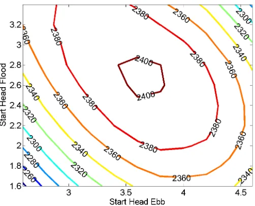
     0 τxy τyy     

, S =

     qs

+hf v+gh(Sbx−Sf x)

−hf u+gh(Sby−Sf y)



(17)

where u,v are the depth-averaged horizontal velocities in the xand y

direc-368

tion, respectively, h is the total water depth, and qs is the source discharge

369

per unit area. The variables τxx, τxy, τyx and τyy represent components of

370

the turbulent shear stresses over the plane, and f refers to the Coriolis

ac-371

celeration. Here the bed and friction slopes have been denoted for thex and

372

y directions as Sbx, Sby and Sf x,Sf y respectively.

373

For coastal ocean models, when solving either the 2D SWE or the

hydro-374

static or non-hydrostatic forms of the 3D Navier-Stokes equations, the first

375

decision generally made is whether the domain in question can be adequately

376

described at a discrete level using a structured mesh, or if the flexibility

af-377

forded by an unstructured mesh is desired. The latter is particularly useful

378

when accurate representation of complex geometries is required, and/or

dras-379

tically different spatial mesh resolution is desired within a single

computa-380

tional domain [50]. A key decision is then often whether open source versus

381

proprietary software is used, and in the case of unstructured meshes whether

382

a finite volume or finite element based discretization approach is employed.

383

For the solution of the governing equations, previous studies have applied

384

a variety of coastal models including ADCIRC [35], Telemac-2D [9], EFDC

385

[32, 51], as well as in-house research-focused software [24, 30].

386

A common aspect in all of these approaches is the manner in which water

387

bodies either side of the impoundment are linked numerically, given that at

388

different times of the lagoon operation they may be completely disconnected,

389

and at others linked through sluices and turbines. A domain decomposition

390

based technique has been the standard approach employed to simulate tidal

391

lagoon operation at a field-scale state [24, 29, 30, 32, 33, 37, 46, 51, 52].

(18)

This technique is implemented using two (or more in the case of multiple

393

impoundments) sub-domains: one upstream, and another downstream of the

394

impoundment. Open boundaries connecting the sub-domains are specified

395

in the region of flow control structures, i.e. turbines and sluice gates.

Sub-396

domains are then dynamically linked using available information regarding

397

the behaviour of hydraulic structures, such as tidal turbine hill charts as with

398

simplified 0D approaches (Section 3.1). Dedicated details for the

represen-399

tation of tidal lagoons in a SWE model and the conservation of mass and

400

momentum through hydraulic structures are expanded in Angeloudis et al.

401

[52].

402

Three-dimensional studies generally commence with an extension of the

403

2D approach to include a number of vertical layers which, while having been

404

applied to other coastal engineering applications, are yet to be applied to

405

the regional scale modelling of tidal range structures. An expansion to 3D

406

layered methods would produce an appreciation of the three-dimensional

con-407

ditions generated by the hydraulic structure-induced water jets. In turn, and

408

subject to the substantial growth in the required computational resources,

409

classical 3D hydrodynamic CFD (computational fluid dynamics) approaches

410

could yield even greater insight. At present, these are only generally

ap-411

plicable for smaller scale hydraulic engineering applications, due to current

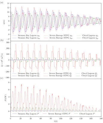
412

limitations of computational resources, including storage. The use of

multi-413

scale unstructured meshes can of course blur this distinction, but one needs

414

to keep in mind the variations in time scales and the need to parameterise

415

different turbulent processes. In fact, the expansion to fully 3D modelling of

416

tidal barrage/lagoon operations has been scarcely reported to date. At the

(19)

time of writing, this has been limited to the CFD modelling of

laboratory-418

scale flows expected downstream and upstream of barrages [e.g. 53, 54, 55].

419

However, 2D models are generally accurate for predicting water levels, and

420

so for most applications, particularly resource assessments, the complexity

421

offered by a 3D model is often not required.

422

3.4. Observations and validation 423

The main types of data used to parameterize and force numerical models

424

are bathymetry and boundary conditions. There are many online sources of

425

bathymetry that are suitable for model setup such as GEBCO (global 1/2

426

arc-minute grid) and EMODnet (European 1/8 arc-minute grid). However,

427

in many circumstances it may be necessary to complement such datasets

428

with local accurate high-resolution survey data, such as LiDAR or

multi-429

beam data, particularly in the inter-tidal. Although many tide gauges exist

430

around the world, providing accurate time series of water surface elevations

431

over many decades, often such datasets do not coincide with model

bound-432

aries, or are unsuitable for boundary forcing (e.g. if there are large changes

433

in amplitude and phase along a 2D boundary). Under such circumstances,

434

global or regional tidal atlases are therefore used to generate boundary

condi-435

tions. One such resource, FES2014 [56], provides both amplitude and phase

436

of surface elevations and tidal currents for 32 tidal constituents at a (global)

437

grid resolution of 1/16×1/16◦.

438

Although it is not possible to validate a model of a lagoon prior to

con-439

struction, it is possible to validate a hydrodynamic model in the absence of

440

a lagoon. Confidence in the hydrodynamic model, along with subsequent

441

rigorous parameterization of the tidal lagoon, therefore provides a tool that

(20)

can be used to explore various tidal range schemes and operating scenarios

443

prior to substantial financial investment.

444

Generally, a thorough understanding of the resource requires that a time

445

series of the free surface is analysed and split into its astronomical

compo-446

nents (e.g. principal semi-diurnal lunar (M2) and solar (S2) constituents),

447

and it is the amplitude and phase of these constituents that forms the

ba-448

sis of model validation. However, in many circumstances, for example for

449

regions or time periods that experience significant non-astronomical effects

450

(e.g. surges), the actual time series can be used to assess the skill and

accu-451

racy of the numerical simulation.

452

4. Tidal range resource

453

4.1. Theoretical global resource 454

The analysis described below estimates the global annual theoretical tidal

455

range resource to be around 25,880 TWh, based on reasonable thresholds for

456

energy output and water depth. However, the resource is confined to a few

457

coastal regions (covering 0.22% of the World’s oceans). In fact, the majority

458

of the resource is distributed across eleven countries.

459

Our global resource characterization is based solely on annual sea surface

460

elevations and water depths. The FES2014 tidal dataset was used, which

461

provides tidal elevations (amplitude and phase) at a consistent 1/16◦×1/16◦

462

global resolution. FES2014 is the latest iteration of the FES (Finite Element

463

Solution) tidal model, and is a considerable improvement on FES2012,

par-464

ticularly in coastal and shelf regions. Water depths were provided by the

465

GEBCO-2014 gridded bathymetry dataset (www.gebco.net), available on a

(21)

1/120◦ ×1/120◦ global grid (which was resampled here to a 1/16◦×1/16◦

467

grid to match the FES2014 grid points), and referenced to mean sea level.

468

For each 1/16◦×1/16◦ grid cell, an annual elevation time series was

con-469

structed (using T TIDE; [57]), based on the following 5 tidal constituents:

470

M2, S2, N2, K1, and O1. For each time series, the tidal range (H) of

consec-471

utive rising and falling tides were calculated, allowing the annual potential

472

energy (P E, per m2_{), to be calculated as follows:} 473

P E =

n

X

i=1

1 2ρgH

2

i (7)

where the subscript idenotes each successive rising and falling tide in a year

474

(n ≈1411),ρ is the density of seawater, andg is acceleration due to gravity.

475

The resulting contour map of global potential energy density (in kWh/m2₎ 476

is shown in Fig. 2.

477

Some assumptions have been made about areas that are suitable for

la-478

goon developments, and we have calculated how much energy there is in just

479

these areas. The true limit of any development will be when the energy

480

yield does not increase the financial return sufficiently compared with the

481

development and running costs (Section 5.2). Here, we assume a minimum

482

acceptable annual energy yield of 50 kWh/m2 _{(based on the energy yield} 483

from a constant tidal range of 5 m), and also a maximum water depth of 30

484

m (since construction costs of the embankment would likely be prohibitive in

485

deeper waters). Applying these criteria, the global annual potential energy is

486

approximately 25,880 TWh; distributed across the coastal regions of eleven

487

countries, as detailed in Table 3.

488

However, for the majority of the year, the largest theoretical resource,

(22)

the Hudson Bay area, contains substantial sea ice (http://nsidc.org/) and

490

steep bathymetric gradients (i.e., the resource in water depths less than 30 m

491

is constrained to the near coastal strip); and would therefore be impractical

492

to exploit. This region is also rather isolated from a demand perspective.

493

Sea ice is also prevalent in Alaska [58] and northern Russia [59], where we

494

calculated significant potential energy. However, lagoons can be designed to

495

take account of static and dynamic ice loads on the structures. Taking into

496

account the impracticality of Hudson Bay for tidal range energy exploitation,

497

the global annual potential energy is approximately 5,792 TWh. Generally,

498

regions with desirable characteristics, i.e. regions where the tidal wave is

499

amplified due to resonance, are limited, and indeed 90% of this resource is

500

distributed across the coastal regions of just five countries, as shown in Table

501

3: Australia, Canada, UK, France, and the US (Alaska).

502

4.2. Theoretical resource of the European shelf seas 503

For more detailed analysis, we focus on the resource of the northwest

504

European shelf seas (NWESS), since this is a region that includes existing

505

(La Rance) and proposed (Swansea Bay) tidal range schemes (Section 2),

506

in addition to hosting around a quarter of the global theoretical resource

507

(Table 3). In order to estimate the NWESS tidal range resource, the 3D

508

ROMS model (Regional Ocean Modeling System) was used to simulate tidal

509

elevations, and subsequently the potential energy in both the flood and ebb

510

phases of the tidal cycle. The model domain extends from 14◦ W to 11◦ E,

511

and 42◦ N to 62◦ N, but the region analysed is shown in Fig. 3. The domain

512

was discretised in the horizontal using a curvilinear grid, applying a variable

513

longitudinal resolution of 1/60◦(0.87-1.38 km), and a fixed latitudinal

(23)

tion of 1/100◦ (∼1.11 km). The bathymetric grid is based on GEBCO global

515

data (www.gebco.net) at 1/120◦ resolution. The vertical model grid consists

516

of 10 layers distributed according to the ROMS terrain-following coordinate

517

system. The open boundaries of the model were forced by tidal elevation

518

(Chapman boundary condition) and tidal velocities (Flather boundary

con-519

dition), generated by 10 tidal constituents (M2, S2, N2, K2, K1, O1, P1, Q1,

520

Mf, and Mm) obtained from TPX07 global tide dataset at 1/4◦ resolution

521

[60]. The validation procedure for elevations, based on harmonic analysis

522

performed at 20 tide gauges distributed throughout the domain, produced

523

scatter indices (SI)3 of <8% and <6% for M2 and S2 amplitudes,

respec-524

tively. Further information about the model set up and validation can be

525

found in Robins et al. [61]. Tidal analysis from a 30-day simulation was

526

used to calculate the following 5 dominant tidal constituents, which were

527

used to construct annual elevation time series at each model grid cell: M2,

528

S2, N2, K1, and O1. Following the method outlined in Section 4.1 and using

529

Eq. 7, the annual energy yield (in kWh/m2) over the northwest European

530

shelf was calculated (Fig. 3).

531

Here, we assume a range of minimally acceptable annual energy yields

532

and also a maximum water depth of 30 m. Based on Tidal Lagoon Power’s

533

planned scheme in Swansea Bay, the lagoon has a surface area of 11.7 km2

534

and a PE of approximately 84 kWh/m2 _{(i.e. a total PE of around 1 TWh)}4_. 535

Other lagoon schemes typically have an annual yield of 60 kWh/m2, and

536

the energy yield based on an M2 amplitude of 2.5 m is approximately 50

537

(24)

kWh/m2_. 538

If we assume initially that exploitable areas are those with water depths

539

<30 m and an annual yield above 50 kWh/m2_{, then approximately 31,415} 540

km2 of sea space (landward of the black contour lines in Fig. 3) is exploitable

541

throughout the NWESS, which equates to a total potential energy of 1,261

542

TWh per annum; 683 TWh per annum (54%) of which is found in UK

wa-543

ters, with the remaining 578 TWh per annum (46%) found in French waters.

544

These estimates are similar to those calculated from the global analysis

(Sec-545

tion 4.1), although the more detailed analysis here produces a 14% lower

546

resource than the global estimate, due to the improved model resolution. To

547

put these values into context, annual demand for electricity is around 309

548

TWh in the UK, and the UK theoretical tidal range resource is about double

549

this.

550

By increasing the threshold to 60 kWh/m2, the exploitable sea space

551

reduces by 18% (to 26,682 km2_{; areas landward of the red contour lines in Fig.} 552

3), but the resource decreases only slightly to 1,154 TWh per annum; 53% of

553

which is found in UK waters, with the remaining 47% found in French waters.

554

Increasing the threshold yield further to 84 kWh/m2(the PE of Swansea Bay

555

lagoon) reduces the total resource to 832 TWh per annum (now with 44%,

556

i.e. 366 TWh, found in UK waters). Based on our criteria, the theoretical

557

resource is concentrated along the UK coasts of Liverpool Bay, the Severn

558

Estuary & Bristol Channel, the Wash, and southeast England. In France,

559

the resource is located along the northern coasts of Brittany and Normandy

560

(Fig. 3).

561

To put the above resource estimates into further context, the total M2

(25)

energy flux onto the European shelf has been estimated using models and

563

satellite altimetry to be approximately 250 GW [62, 63], which equates to an

564

annual energy yield of 2,190 TWh. However, the total potential energy might

565

be higher than this, because the potential energy is moving around the system

566

all the time and, hence, it is difficult to obtain a definitive theoretical value.

567

If we take energy out of the system via lagoons, it is presently unclear how

568

this will affect the energy dissipation on the shelf and the energy flux across

569

the shelf edge (i.e. influencing other energy systems globally). Further, since

570

discrete lagoons within the European shelf may interact with one another,

571

it is possible that the theoretical resource would alter from that calculated

572

above (Section 5.4).

573

Our resource estimates are based on theoretical energy yields, which are a

574

function of tidal range and water depths. In practice, the technical resource

575

will be considerably lower than the above theoretical estimates. For example,

576

Prandle [8] estimated that approximately 37% of the theoretical resource was

577

available for dual (flood and ebb) schemes.

578

Of course, not all areas with sufficient yield can be exploited, due to

prac-579

tical difficulties with development at this scale, together with political and

580

practical constraints regarding planning. It is also unlikely that, in the near

581

future, lagoon designs would consider water depths greater than

approxi-582

mately 20 m (Mike Case, Tidal Lagoon Power; Pers. Comm.), although

bar-583

rage designs might. Therefore, our resource calculations in regions suitable

584

for lagoons should be considered an over-estimate. Moreover, it is unlikely

585

that lagoon designs at this scale could maintain the high tidal amplification

586

near to shore. For instance, if a very large lagoon was developed, then the

(26)

tidal range within the lagoon would be reduced to approximately that at the

588

lagoon wall. Using models, lagoon optimization studies may reveal that

sev-589

eral smaller strategically sited lagoons within a region could lead to a greater

590

energy yield than one larger lagoon.

591

4.3. Non-astronomical influences on the resource 592

The previous analysis, and indeed most studies of tidal range resource,

593

assume only astronomical tides, and typically apply harmonic tide theory

594

to predict water levels. However, the tidal resource can be influenced by

595

non-astronomical effects, namely storm surge. Hence, potential reliability

596

problems within tidal range energy schemes could be due to storm surges

597

[64], as negative surge events reduce the tidal range, with the converse

oc-598

curring during positive surge events. Tide-surge interaction, which results

599

in positive storm surges being more likely to occur on a flooding tide [65],

600

may also reduce the annual tidal range energy resource estimate. In a recent

601

paper by Lewis et al. [64], water-level data at nine UK tide gauges suitable

602

for tidal-range energy development (i.e. where the mean tidal amplitude

ex-603

ceeds 2.5 m [23]) were used to predict tidal range power with a 0D model.

604

Storm surge affected the annual resource estimate by between -5% to +3%,

605

due to inter-annual variability in the 12 year tide gauge records. However,

in-606

stantaneous power output was significantly affected (Normalised Root Mean

607

Squared Error: 3−8%, Scatter Index: 15−41%) [64]. Therefore, a prediction

608

system [e.g. 66, 67] may be required for any future electricity generation

sce-609

nario that includes a high penetration of tidal-range energy; however, annual

610

resource estimation from astronomical tides alone appears sufficient for

re-611

source estimation, because uncertainties in resource assessment due to design

(27)

and modelling assumptions appears greater.

613

4.4. Long timescale changes in the tidal range resource 614

Mean sea-level rise, which occurs incrementally over decadal timescales,

615

results from variations in ocean mass and ocean water density (thermosteric

616

and halosteric changes) caused by global warming and subsequent ice melt,

617

due to changes in anthropogenic or natural land-water storage and from

618

changes in ocean circulation [68]. Global mean sea level is likely to rise by

619

0.44−0.74 m (above the 1986−2005 average) by 2100 [69]. However, there

620

remain large model uncertainties in sea-level rise projections, in particular

621

when predicting the volume contribution from melting ice sheets [69], and

622

projections could increase to 1.9 m [70].

623

Future mean sea-level rise is likely to affect tidal dynamics by

impact-624

ing on the position of amphidromic points and by changing resonant effects

625

on shelf seas [71, 72, 73, 74], with variation in regional (relative) sea-level

626

changes due to ongoing local and far-field isostatic effects [69, 75]. In the

627

UK, observed MSL rise is broadly consistent with global MSL rise [76]. A

628

study by Ward et al. [72] indicated that projected sea-level rise over the

629

21st century is likely to alter both tidal amplitudes and tidal phases. Such

630

changes in sea levels will influence the tidal range resource, although

uncer-631

tainties in modelling the potential impacts are significant. A preliminary

632

study by Robins et al. [77] investigated how these changes are likely to affect

633

the theoretical resource at the top eight tidal range sites around the UK.

634

There was generally an increase in tidal range at these sites (1 −3%,

re-635

sults not shown), causing the resource capacity to increase. However, when

636

the aggregated power density from multiple potential lagoon locations was

(28)

considered, tidal phase shifts tended to reduce the base-load capacity of the

638

aggregated system. In one example future scenario, simulated sea-level rise

639

clearly predicted an increased aggregated resource capacity, although the

cor-640

responding phase shifts led to reduced resource minima, which is a potential

641

consideration for firm power generation. This preliminary work can be

im-642

proved upon by considering how the feedbacks of a tidal energy extraction

643

site on the local tidal dynamics (i.e. on the resource itself) might vary with

644

changing sea levels [e.g. 72, 73].

645

4.5. Socio-techno-economic constraints on the theoretical resource 646

It is clear that not all potential tidal range sites will be developed to

647

their fullest extent. Large infrastructure projects of this type will always be

648

modified in societies where there is a democratic involvement in the planning

649

process by the local population. For example, a factor in the lack of progress

650

of the Severn barrage has been the concern of decision makers about the

pub-651

lic acceptability of the scheme. An important element of public acceptability

652

is the impact of a scheme on the local environment. This is part of planning

653

law in many countries, and within the EU is legislated by the overarching

654

Marine Strategy Framework Directive (MSFD) [78]. The most recent formal

655

review of the Severn Barrage examined environmental concerns, and

con-656

cluded there would be major impacts on migratory fish and other protected

657

species [79]. Therefore, if the UK government were to approve such a scheme,

658

it would be vulnerable to a legal challenge under the MSFD. Any lagoon in

659

the Severn would have to consider the same receptor species and habitats

660

as the barrage, and may have to provide compensatory habitat, increasing

661

the capital cost of the project. As an example of environmental concerns

(29)

limiting the resource capture of a project, even though the Swansea Bay

la-663

goon has gained (partial) planning consent, the shape is deliberately placed

664

to minimise interference with the Tawe and Neath rivers [80].

665

The coastal zone provides humans with extensive ecosystems services, and

666

include visual amenity, including coastal seascapes [81]. Swansea Bay lagoon

667

is an example of siting a structure to mitigate visual impacts; the structure is

668

located in the northern part of Swansea Bay, next to the dock infrastructure,

669

and away from the desirable residential areas and tourist seafront located to

670

the west of the bay [80].

671

Many European countries are developing Marine Spatial Plans [82], so

672

that they have a strategic long term oversight of economic activity in the

673

oceans. The shipping industry has an historic presumption of safe navigation

674

to port, and most coastal waters have navigational zones and marked shipping

675

channels. The large scale development of lagoons could interact with these

676

channels, and any perceived impediment to navigation would be contested

677

robustly. A Marine Spatial Plan attempts to resolve these differences at

678

an early stage; however, the consequences are that lagoon shapes and sizes

679

will evolve from the most economically desirable geometry due to harbour

680

access. When other uses of the sea are taken into account, including marine

681

aggregates, offshore wind, and aquaculture, the space available for lagoons

682

could be significantly constrained. One solution could be the Multiple Use

683

of Space (MUS), with the inside of the lagoon providing an area that is

684

protected from wave action and consequently suitable for a number of other

685

uses. The MarIBE project [83] considered a number of MUS projects, and

686

proposed suitable business models for future exploitation. In particular, the

(30)

combination of aquaculture and a lagoon was investigated [84].

688

A previous project [85] considered a number of factors related to

deploy-689

ment of tidal stream turbines in the Severn Estuary, including a preliminary

690

navigational risk assessment. Although the study is not directly applicable

691

to lagoon deployment, there were two key findings. Firstly, early engagement

692

with local pilots established that the “best” location for turbines from a

re-693

source perspective was co-incident with an area of sea that is key to vessel

694

logistics. Secondly, the majority of the channel is 20−30 m relative to LAT5,

695

and larger container vessels are routinely 16 m draft, making large areas of

696

the channel practically unusable for the largest vessels. Applying this result

697

to all areas with high tidal range, the application of good spatial planning

698

could lead to the deeper channels available for vessels, and shallower areas

699

designated for lagoon technology.

700

Building a lagoon is a significant item of infrastructure, and good port

fa-701

cilities are essential, in a similar way to the investments in round 3 wind farm

702

construction on the east coast of the UK [86]. Tidal Lagoon Power Plc

com-703

missioned a supply chain study that outlines the infrastructure requirements

704

[87]. Locations with theoretical resource but devoid of suitable ports in close

705

proximity may not be practical for this reason. The construction techniques

706

used also have a relevance to the port facilities required. La Rance barrage

707

made use of a Bund construction [88], and hence was effectively a

conven-708

tional land based civil engineering construction. However, such methods take

709

a considerable amount of time, and may not be suitable for larger lagoons.

710

(31)

Therefore, concrete caissons have been under consideration for a considerable

711

period of time. Clare [89] considered the caisson requirements for the 1980s

712

STPG Severn Barrage, which proposed the use of the majority of deep water

713

ports in the UK, together with towing large caissons over considerable

dis-714

tances. Finally, and importantly, a lagoon must of course be able to export

715

power to the grid, and so proximity to a suitable grid connection is a key

716

constraint.

717

5. Optimization

718

There are two main categories of tidal lagoon optimization. The first

719

is optimization of the operation of the turbines and sluices to maximize

720

the energy yield from the lagoon, and the second is optimizing the overall

721

economic design of the lagoon to minimize the cost of energy. The academic

722

literature has focused on energy optimization, while industry tends to focus

723