Shape optimization with surface mapped CPPNs

Daniel Richards and Martyn Amos

IEEE Transactions on Evolutionary Computation.

http://dx.doi.org/10.1109/TEVC.2016.2606040

Abstract—Shape optimization techniques are becoming increasingly important in design and engineering. This growing significance reflects the need to exploit advances in digital fabrication technologies, and the desire to create new types of surface designs for various engineering applications. Evolutionary algorithms offer several key advantages for shape optimization, but they can also be restricted, especially as design problems scale up in size. A key challenge for evolutionary shape optimization is to overcome these challenges in order to apply evolutionary algorithms to large-scale, "real-world" engineering problems. This paper presents a new evolutionary approach to shape optimization using what we call “surface-mapped CPPNs”. Our method outperforms a state-of-the-art gradient-based method on a simple benchmark problem, and scales well as degrees of freedom are added to the design problem. Our results demonstrate that surface-mapped CPPNs offer practical ways of approaching large-scale, real-world engineering problems with evolutionary algorithms, opening up exciting new opportunities for engineering design.

Index Terms—Shape optimization, engineering design, generative encodings, optimization methods, CPPN-NEAT.

I.

INTRODUCTION

The recent proliferation of digital fabrication technologies

(such as 3-D printing) has generated growing interest in

high-performance

shell structures

and mechanically motivated

surface designs [1]-[7].

Shape optimization

techniques are a

central component of this research field, and are used to

produce high-performance designs according to precise

requirements.

Shape optimization consists of three key elements. First,

geometry

of a 2-D or 3-D design is modeled so that all degrees

of freedom are identified and parameterized. Second, the

design is

meshed

(i.e., discretized) to ensure it is suitable for

analysis and simulation (e.g. flow solver or structural

analysis). Finally, an

optimization

process is used to

manipulate the parameterized mesh design according to some

objective function. Today, both gradient-based treatments and

evolutionary algorithms are used in shape optimization.

Manuscript received April 22, 2016. This work was supported in part by funding from Manchester Metropolitan University.

D. Richards is with Imagination Lancaster and the Data Science Institute at Lancaster University, LA1 4YW, UK. He was previously with the Department of Computing, Mathematics, and Digital Technology, Manchester Metropolitan University. (e-mail: [email protected]).

M. Amos is with the Informatics Research Centre, Manchester Metropolitan University, M1 5GD, UK. (e-mail: [email protected]).

Gradient-based methods are used across a wide range of

structural optimization problem domains, including shape

optimization, [1], [2], [8], [14], [34]-[38]. The general

principle is to iteratively simulate the mechanical performance

of an object, perform a gradient sensitivity analysis, and

determine a series of geometric adaptations that will improve

the engineering design in relation to the objective function [8].

When the design problem is (or can be made) convex,

gradient-based methods work well, and converge to

optimal

solutions in good time.

Evolutionary algorithms

(EAs) are also applied to shape

and structural optimization, particularly in fields such as

aeronautical and aerospace engineering (see [9] for an

extensive review). Aeronautical applications of shape

optimization techniques include next-generation airplane

wings [10] and structurally robust monocoque shells [4], but

these methods are also now being applied to architectural

design in order to create large-scale, efficient, free-form

structures [2]. This broadening in application is largely due to

the increased availability of easy-to-use software packages,

combined with affordable new fabrication processes [11].

As outlined in [9], EAs offer several key advantages for

shape and structural optimization, compared to gradient-based

numerical optimization methods. Two key advantages are (A)

the ability to deal with

complex multimodal design spaces

and

highly nonlinear objective functions

(which are common in

real-world problems), and (B)

ease-of-use

by designers and

non-specialist engineers.

However, these advantages come at a cost. EAs are more

computationally expensive than gradient-based methods, due

to the bottleneck imposed by having to evaluate populations of

solutions. Additionally, EAs do not

guarantee

convergence to

optimal solutions and they often scale poorly. Consequently,

evolutionary approaches are often limited to exploring

relatively trivial benchmark problems with coarse

discretization (i.e., with few degrees of freedom) and

described using relatively few design variables.

This inability of EAs to deal with large-scale structural

optimization problems and generate useful solutions within

acceptable timeframes has led to criticism [12]. Consequently,

state-of-the-art

shape optimization methods generally

comprise

gradient-based

approaches that employ a variety of

sophisticated filtering techniques that help to convexify noisy

search spaces and ensure successful convergence to optimal

solutions [1], [2], [12]-[14].

In both gradient-based and evolutionary approaches, the

way that geometry is modeled and

parameterized

plays a

crucial role in the optimization process. Specifically, designs

described by too few

parameters

(i.e. degrees of freedom),

Shape Optimization with

Surface

-

Mapped CPPNs

tend to converge quickly to sub-optimal solutions, due to the

low-resolution nature of the parameterization. On the other

hand, designs defined by relatively many parameters (i.e. more

degrees of freedom) can often converge to superior solutions,

due to the expanded space of possible shapes. However, in

order to do so, they usually require many more evaluations,

and thus use significantly more computational resource in the

process.

In order to address this challenge in practice, designers

often

manually test various different parameterizations of

problems in order to find the best solutions [13]. However,

this process is time consuming and labor intensive, and is

further compounded for evolutionary models, which typically

need many more evaluations to solve similar problems.

Indeed, this scalability challenge usually renders evolutionary

methods unusable when shape optimization problems are

described by many degrees of freedom [9], [12]. One route

towards scaling up EAs for large-scale shape optimization

problems

may lie in alternative chromosome encodings

[9],

but further work is required.

In this paper, we present a new (gradient-free) evolutionary

method, which we call surface-mapped CPPNs, and which is

able to deal with large shape optimization problems with many

degrees of freedom.

We first show that our approach can produce solutions with

mechanical performance that is superior to that of solutions

produced with state-of-the-art gradient-based methods, and

then demonstrate that our method eliminates the mathematical

challenge of scalability. To support these claims, our first

experiment uses a well-known benchmark problem to compare

the physical properties of solutions found by both

state-of-the-art gradient-based methods and surface-mapped CPPNs. We

validate these results to show that our evolved solutions are

both reliable and mesh-independent. The second experiment

then tests our surface-mapped CPPN on the same benchmark

problem, but this time uses eight different parameterizations.

This demonstrates that instances do not become more difficult

to solve as more degrees of freedom are added to the design

problem. When combined, these results demonstrate a

powerful new approach to shape and shell optimization that is

especially well-suited for exploiting digital fabrication

technologies in high-performance engineering design.

The paper is organized as follows: we begin by discussing

related work. We then outline our new method, describe the

base experiment and validate these results, before presenting a

second experiment to demonstrate the scalability of our

approach. Finally, we conclude with a discussion of our

results, and highlight further opportunities for development.

II.

BACKGROUND

EAs offer several key advantages for engineering domains, but

further work is needed to develop

alternative chromosome

encodings

if they are to be competitive with state-of-the-art

gradient-based methods [9]. Typically, chromosomes used in

shape optimization consist of vectors of either real or binary

numbers that describe transformations of individual vertex

positions in 2-D or 3-D geometries (e.g. [1], [4], and [15]).

The problem with this approach is that as designs increase in

size and complexity, the chromosome encodings also become

much larger (due to the direct nature of the one-to-one

mapping) and this significantly expands the search space,

making it harder to find good solutions. Real-world shape

optimization problems can easily comprise thousands of

vertices, and encoding schemes are needed that allow for more

effective search of these vast spaces. This scalability challenge

is well-known in in the evolutionary computing community

[16] and is the subject of much research. To improve how EAs

perform on large-scale problems, several techniques may be

employed.

Firstly, to limit computational expense of simulating large

populations of possible solutions, variants of

Evolutionary

Strategies are often used [9], [17]. These techniques

demonstrate good convergence speed with small population

sizes, and in doing so significantly improve how EAs scale.

However, they do not

eliminate the underlying problem, and

are thus still susceptible to scalability challenges on

large-scale problems [12].

A second approach to improving scalability is to limit the

dimensionality of the search space. This may be achieved by

exploiting

a priori domain-specific knowledge of the design

problem, and thus identifying only the important parameters to

use in the shape optimization procedure. For example, when

optimizing solutions that require fine-grained meshes, a

common approach used by both EAs and gradient-based

methods is to apply a series of

control points to the original

geometry, and define the position of each individual mesh

vertex in relation to changes to a smaller number of specific

control points. In this way, the shape optimization algorithm

manipulates the positions of only the control points, allowing

for a significant reduction in the dimensionality of the search

space [18], [19]. The benefit of optimizing compact

parameterizations lies in the fact that the system generally

converges quickly. However, for this approach to work, the

correct identification and parameterization of all control

points are crucial. Consequently, for problems where

comprehensive domain knowledge is not available in advance

(which is usually most of them) this method has limited

practical value.

required in order to manually test and calibrate this new

system parameter for each new problem, which is time

consuming, labor intensive, and impossible for non-specialists.

(B) It is unclear how well this approach works on highly

non-convex

problems, which are characterized by deceptive

design spaces.

(C) The ability of this approach to scale up to extremely

large problems has yet to be demonstrated. To date, existing

work using this approach has been limited to the addition of

20-30 parameters to solutions over the course of an

optimization process [17], [20]-[21]. But real-world problems

can easily contain thousands of degrees-of-freedom, and this

number is growing alongside the geometric freedom offered

by advanced fabrication technologies [2], [5], [9].

Ultimately, adaptive parameterizations provide a trade-off

whereby a designer may make an educated initial guess as to

which parameters are critical, and then use the algorithm to

adjust this identified parameterization throughout the

optimization process. However, as we argue throughout this

paper, significant progress in this area can only be made when

the parameterization of geometry is

independent

of the

dimensionality of the search space.

Outside the scope of typical shape optimization methods,

the area broadly defined as

generative and developmental

systems

focuses on the capacity to evolve complex solutions

from extremely compact encodings [22]. This paper will

demonstrate that specific ideas, which have emerged from this

area in recent years [23]-[28], have the potential to

significantly advance engineering design through powerful

new shape optimization techniques.

Our central insight involves changing the way that shape

optimization problems are

conceptualized

. The key is thinking

in terms of

patterns

instead of

points

. The traditional view of

shape optimization problems is to view solutions as large

collections of

points

that are individually adjusted in order to

improve the performance of a design. The problem with this

perspective is that each point is usually described by an

individual optimization variable, and this means that solutions

with

many

points are required to solve high-dimensional

problems.

However, if we step back and view solutions as

functional

patterns

painted across surface-conformed canvases, then the

problem becomes conceptually much easier to solve. Indeed,

from this perspective, the resolution of the canvas (i.e. number

of vertices on the surface) may be independent of the

functional

description of the pattern (i.e. a mathematical

function). This means that the traditional scalability problem

can be eliminated, because the

parameterization

of the

problem and the

dimensionality

of the search space are no

longer explicitly linked.

To shift our thinking from the manipulation of individual

points to instead

painting

functional patterns across geometry,

we build on a rich body of work relating to the

NEAT

(Neuroevolution of Augmented Topologies) model [23] and

CPPNs

(Compositional Pattern Producing Networks) [24]

[25], [26].

In 2007, Stanley [24] demonstrated that CPPNs can paint

functional patterns across 2-D (pixel-based) canvases and be

evolved with NEAT [23] to discover novel pictures. This idea

is perhaps best demonstrated with Picbreeder [25], an online

tool where users collaboratively evolve populations of 2-D

images. Following these 2-D demonstrations, Clune and

Lipson [26] extended the idea of Picbreeder to evolve 3-D

objects that can be fabricated with 3D printing technologies.

In recent years, CPPN-NEAT has been used for a variety of

applications, including evolving virtual [29], [30] and physical

[31] creatures with diverse locomotive behaviors and dynamic

properties [32], topology optimization [33], simulation of

multi-material objects that that exhibit higher-level behaviors

such as specific deformations of 3-D beams [34] and

vibrational frequencies [35], and evolution of efficient truss

designs [36].

We suggest that CPPN-NEAT methods offer vast potential

for shape optimization. However, in order to unlock the power

of CPPNs for real-world optimization problems, it is necessary

to resolve a key limitation of existing approaches. 3-D CPPN

models have, to date, been almost exclusively used to control

properties of volumetric pixels (or “voxels”) within traditional

Cartesian (x,y,z) grids. From an engineering perspective, this

approach has limited

practical

value. This is because

real-world engineering problems typically require manipulation of

pre-defined

shapes and geometries, which are also subject to

various physical constraints.

To address this challenge, Clune

et al

. [37] created a novel

method of “seeding CPPNs” with geometric information

associated with predefined shapes. The approach begins with a

normal 3-D CPPN setup, whereby a 3-D array of voxels is set

within a Cartesian grid, and a CPPN defines the property of

each voxel as a function of its Cartesian (x,y,z) coordinate

values. The key innovation of this approach (as described

[37]) is to place a 3-D shape within the Cartesian voxel grid,

and to then add an additional input to the CPPN, which inputs

the distance between each voxel and the nearest point of the

3-D shape. By seeding a CPPN with geometric information

about a predefined shape, Clune

et al

. show that it is possible

to upload a voxelized version of the original 3-D shape, and

then evolve it using the NEAT algorithm.

This approach to

seeding CPPNs

is potentially valuable for

exploring conceptual 3-D designs. However, from an

engineering design perspective, we argue that it is limited in

specific ways.

A major problem is that designs produced with this method

are often impossible to build (for example, featuring

disconnected parts that "float" in space). Critically, most

engineering design problems demand that specific constraints

are enforced, e.g. all points on the surface of an object might

need to be constrained to only move in one direction, or by a

maximum distance. To our knowledge, seeded CPPNs are

unable to deal with this sort of design constraint.

Another issue specific to shape optimization is that the

geometric patterns and regularities, which feature in many

solutions, are probably expressed much more easily as 2-D

patterns mapped across curved surfaces than as 3-D patterns

which define all solid and void voxels within a larger (and

computationally expensive) 3-D array of voxels. Indeed, the

ability to exploit a

surface-mapped

coordinate system may

provide more useful compositional information relating to the

design problem.

relates to an object in Cartesian space, our approach may be

conceptualized as wrapping a volume around a 3-D object and

then

mapping

all inputs of the CPPN to suit a new

object-based coordinate system.

The first major contribution of this paper is to show how

our approach can unlock the power of CPPNs for real-world

shape optimization problems. The second main contribution is

to show how surface-mapped CPPNs can

scale up

and deal

with truly large-scale problems, thereby eliminating the

long-standing scalability challenge associated with evolving shapes

with many degrees of freedom.

III.

BASE

EXPERIMENT

A.

Methods

CPPN-NEAT has been previously described in detail

[22]-[37] so here we provide only a brief summary, and focus on

how our proposed method differs from existing versions.

CPPNs are similar to neural networks, but the neurons in a

network may contain a

variety

of different activation

functions, and may be evolved with NEAT [23]. CPPNs query

a discretized spatial domain by inputting the

positional

information

(e.g. (x,y,z) coordinates) of each element and

returning values that determine specific

properties

of that

element (e.g. color). Through this process CPPNs can control

grids of pixels and voxels to create 2-D and 3-D patterns.

CPPNs can create a vast array of diverse patterns using

compact encodings, and the patterns produced display

geometric regularities, symmetries and even imperfect

symmetries due to periodic activation functions within the

CPPN (e.g.

cosine

) [24].

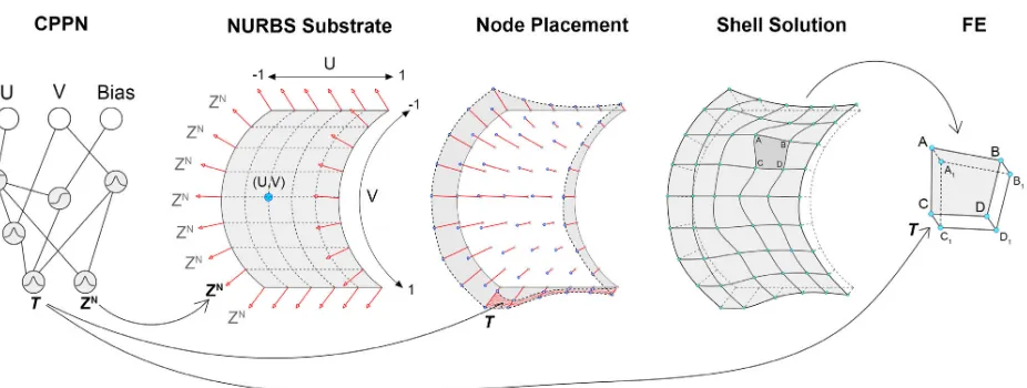
The key difference in our model is that we use CPPNs to

paint patterns across

Non-uniform Rational Basis Spline

(NURBS [38]) surface domains (Fig 1). NURBS surfaces are

commonly used to model geometry in design and engineering

software packages. A useful property of NURBS surfaces is

that any point can be located on the surface using a

relative

(

U, V

) coordinate system that extends from (0, 0) to (1, 1). As

shown in Figure 1, we can exploit this relative coordinate

system to build a new

surface-mapped

domain that is

"clamped" between (-1, -1) and (1, 1). We can then discretize

any NURBS surface, query each point by feeding its (

U, V

)

coordinates into a CPPN, and then use the output value (

Z

_{) as}

the distance by which to move the queried (U,V) point relative

to its surface normal. Following placement of surface nodes,

we mesh the solution to create a shell with specific thickness,

and export this information for structural analysis using a

commercial

finite element analysis

(FEA) solver.

We refer to this approach as

mapping

a CPPN to a

predefined NURBS surface. Our choice of terminology is

intended to provoke analogies with conceptually similar

techniques in computer graphics - specifically, techniques

such as

texture mapping, bump mapping, normal mapping

and

displacement mapping

that are used to

paint

textures across

geometry in computationally efficient ways. Indeed, our

surface-mapped CPPNs operate in a similar manner, allowing

us to paint geometric and material transformations across

geometry, yet they can also be evolved with NEAT to discover

mechanically motivated surface designs.

1)

Benchmark Setup

To test our

surface-mapped CPPNs

, we use the simple

benchmark problem originally proposed in [39], and more

recently extended by [13], to demonstrate the performance of

their sophisticated FE-based parameterization scheme in

combination with the state-of-the-art gradient-based method:

SIMP

(Solid Isotropic Material with Penalization) [40].

We choose this benchmark problem for three key reasons.

First, as discussed by [41], this problem is “highly

non-convex”, and state-of-the-art shape optimization methods

reach local optima defined by an engineer’s initial choice of a

“sensitivity filter size” [13]. Second, this problem has been

widely published in recently years [13], [41]-[44], and

consequently we have good data with which to make

comparative analyses. Finally, this benchmark problem has

over 1,000 finite elements (FE) and comprises 1,736 degrees

of freedom, which makes it challenging to solve with

traditional

gradient-free

methods [12].

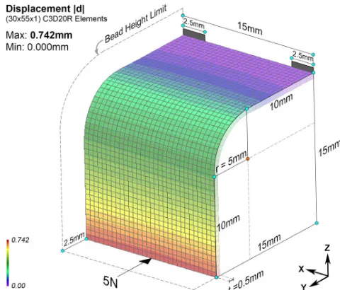
The goal of the benchmark problem is to stiffen a bending

dominated L-shaped cantilever (Fig 2). Stiffening is achieved

by moving FE-nodes relative to the surface normal and

creating structural beads that are subject to a maximum bead

height. The cantilever is made of steel (E=210GPa and v=0.3)

and has a thickness of 0.5mm. The structure is fixed at the top

left and right corners, and is loaded with a single load of 5N,

as shown in Fig. 2. The optimization variables are the set of

heights

of all FE-nodes relative to the surface normal. These

variables are continuous, yet clamped between zero and the

maximum bead height of 2.5mm. The objective is to minimize

displacement experienced at the point on the L-shaped

structure where the 5N load is applied (see Fig 2).

We perform our finite element calculations using the

open-source solver CalculiX, and use C3D20R elements, which are

common across a variety of commercial FEA packages and

perform well in bending. For the shape functions of C3D20R

elements, see [45].

2)

NEAT Setup

We perform 10 independent runs, each with a population of

100, evolved for 160 generations. We use our own Java

implementation of NEAT with the following activation

functions:

Gaussian, Sigmoid, Sine, Cosine

and

Linear,

all

with an equal probability of being selected. We promote 25%

of the population using mutations (i.e. no crossover), and for

the remaining 75% of the population there is an 80% chance

of mutating individuals after crossover. Mutation rates are

0.03 for adding a new node, 0.05 for adding a new link, 0.8 for

perturbing a connection weight, and the probability of

interspecies mating is 0.001. We use a dynamic compatibility

threshold, the target number of species is 8, the initial species

delta is 4, the niche size required for elitism is 5. Finally, the

compatibility coefficients are c1 = 1.0, c2 = 1.0, c3 = 0.5. For

a full description of the NEAT parameters see [23].

3)

Fitness Function

To maximize stiffness of the cantilever, we minimize

displacement experienced at the loading node. We calculate

the magnitude of displacement as:

!

=

(!"

₊

_!

_!"

_+!

_!"

₎

_{!!!!!!!!!!!!!!!!!!!!!!!!!!!!!!!!!!!!!!!!!!!!!!!!!!!!!}

₁

Where:

|d|

is the magnitude of displacement,

ux

is absolute

displacement in the x-axis,

uy

is absolute displacement in the

y-axis, and

uz

is absolute displacement in the z-axis. NEAT is

a maximization algorithm, so we define our fitness function

as:

!"#

1

|

!

|

!!!!!!!!!!!!!!!!!!!!!!!!!!!!!!!!!!!!!!!!!!!!!!!!!!!!!!!!!!!!!!!!!!!!!!!!!!!!!!!!!!!!!!!!!!

(2

)

B.

Results

1)

Comparative Analysis

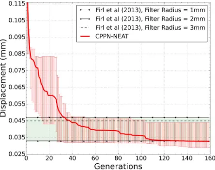
We compare our results with those described in [13], which

uses the (current) state-of-the-art (gradient-based)

Solid

Isotropic Material with Penalization

(SIMP) method with a

sophisticated FE-based parameterization scheme and

sensitivity filter to address the same problem. This method

produces high-performance solutions within about 30

optimization steps. Importantly, by varying the size of the

sensitivity filter radius, the method converges to

different

local

optima. This allows designers and engineers to run the model

several times using a variety of different filter sizes in order to

pinpoint the best performing solutions. The authors of [13]

present results using three different filter sizes: 1mm, 2mm

and 3mm, recording optimized |d| values of 0.047mm,

0.033mm and 0.045mm respectively. These solutions

represent significant improvements over the original geometry

(0.742mm, as shown in Fig. 2). However, we now

demonstrate that our surface-mapped CPPN method produces

solutions with superior mechanical properties.

Figure 3. Performance of 10 runs of our model over 160 generations. Each line shows the best solution in the population at each generation (indicated by a point). 90% of our test runs discovered solutions, which outperformed designs created by Firl et al. [13] with state-of-the-art gradient-based methods.

Figure 4. Mean convergence of the best solution in the population at each generation, over 10 runs. Also shown are the range of best solutions discovered at each generation over the 10 runs.

2)

Model Validation

We argue that our method is able to outperform

state-of-the-art gradient-based methods in this problem domain because

conventional sensitivity filters do not hamper our designs.

Specifically, we think that the sensitivity filters, applied

during gradient-based methods to (uniformly) smooth designs,

actually

prevent

methods from discovering potentially useful

geometric features

. Since our evolutionary (i.e. gradient-free)

approach does not need to calculate sensitivity gradients, it is

not limited in the same way, and can therefore access and

exploit geometric features that gradient-based approaches

cannot. However, it is important to note that sensitivity filters

are a well-established component of shape optimization, and

fulfill multiple functions [14]. Consequently, to support the

claim that our

unfiltered

solutions have superior performance,

we first show that our solutions are valid.

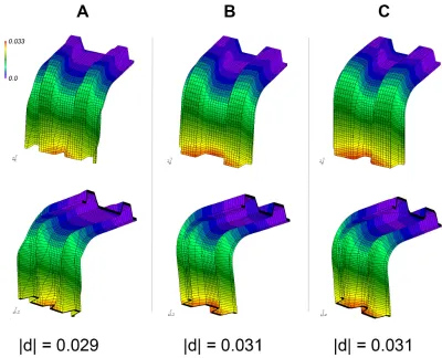
As shown in Fig. 5A, when our FE-nodes move relative to

the surface normal they cause our elements to stretch and

produce slightly irregular meshes. Sensitivity filters are

traditionally applied at this point to smooth mesh geometry

and redistribute nodes, so that the size and shape of all mesh

elements remain as uniform as possible.

This filtering process plays three key roles in gradient-based

methods. Firstly, smoothing helps eliminate noise and ensures

that gradient sensitivities are accurate during sensitivity

analysis calculations. Secondly, the smoothed meshes help

reduce numerical anomalies that can occur in FEA

calculations due to distorted mesh elements. Finally,

smoothing helps produce solutions that are

mesh independent

(i.e. that are not exploiting specific attributes of the

discretization) and return the equivalent physical performance

when simulated with finer meshes [13].

Since our evolutionary method does not require gradient

information, we validate our solutions by showing that they

are (A) not exploiting numerical errors caused by mesh

distortion (i.e. not displaying deceptive physical performance),

and (B) are mesh-independent.

Our FEA calculations use C3D20R elements, which are

common quadratic brick elements with reduced integration

points (2x2x2). C3D20R is a reliable and robust

general-purpose element, and is not susceptible to numerical

instabilities such as hour-glassing and locking phenomena.

Consequently, a simple method of demonstrating validity of

our method is to re-evaluate our final solutions with finer and

more regular meshes (i.e. greater discretization of well-shaped

C3D20R elements), and demonstrate equivalent results.

A novel property of the CPPN encoding is that the solutions

theoretically obtain

infinite resolution

. That is, because CPPNs

paint functional patterns across a NURBS-based substrate, the

designs they encode are not limited to a fixed resolution. In

order to increase the resolution of evolved solutions, we may

simply increase the discretization of the NURBS substrate (in

this case, the L-shaped cantilever shown in Fig 2), and

re-query the CPPN to create high-resolution meshes. However, in

contrast to sensitivity filters, which have a tendency to

“over-smooth” geometric features, increasing the resolution of

solutions discovered with surface-mapped CPPNs can have

the inverse effect of “under-smoothing” evolved features and

revealing geometric properties that were not apparent at the

resolution originally used to optimize the design.

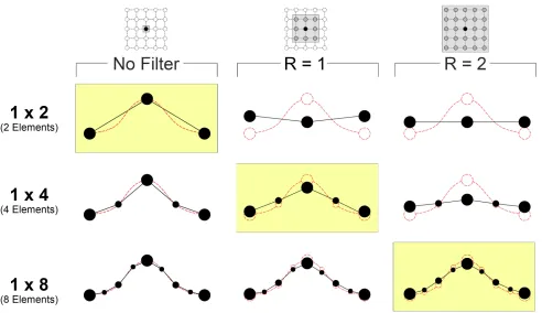
For example, consider a 2-D beam that has been evolved

using our method, and is composed of only two horizontal

finite elements. If the (continuous) CPPN output describes a

Gaussian curve, then the discretized 2-D beam design (1x2

elements) will form an upside down “V” shape (Fig. 6).

However, as we increase the resolution of the design by

subdividing the domain and adding extra elements (e.g. 1 x 4

and 1 x 8), the solution begins to approximate the

CPPN-generated Gaussian distribution, and thus the evolved

upside-down “V” shape is lost.

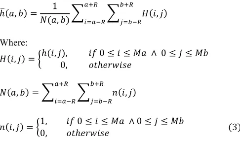
To counteract the tendency to

under-smooth

solutions as

mesh resolution is increased, we can apply a simple Laplacian

smoothing filter (see [46] for an extended description of

Laplacian smoothing). This has two significant effects. Firstly,

the smoothing filter dramatically improves mesh regularity (as

is known from traditional sensitivity filters), but secondly, it

ensures that higher resolution designs closely approximate the

original evolved design. To perform Laplacian smoothing, we

re-query our evolved CPPN and define the height of each node

using the average output of surrounding nodes within a Moore

neighborhood of range,

R

:

ℎ

!,

!

=

1

!

(!,

!

)

!

!,

!

Where:

!

!,

!

=

ℎ(!,

!

_0,

)

,

!!!!!!!!!!

_!!!!!!!!!!

_!"ℎ!"#$%!

!"

!

0

≤

!

≤

!"

!

∧

!

0

≤

!

≤

!"

!!!!!!!

!

!,

!

=

!

!,

!

!!!!!

!!!

!!!!!

!

!,

!

=

_0,

1

,

!"

_!"ℎ!"#$%!

!

0

≤

!

≤

!"

!

∧

0

≤

!

≤

!"

!!!!!!!!!!!!!!!!!!!!

(

3

)

Where:

ℎ

!,

!

is the average (Laplacian smoothed) height,

h

, of node

(!,

!

)

,

R

is the Moore neighborhood range, and

Ma

and

Mb

are the maximum number of nodes in the

a

and

b

dimensions of the mesh grid, respectively.

As shown in Fig. 6, the success of this method, when

applied to CPPN generated outputs, relies on careful

coordination between the Moore neighborhood range,

R

, of

the Laplacian smoothing filter and the increased resolution

size. For example, if we apply the Laplacian filter directly to

the initial (1 x 2) 2D beam design (i.e. without increasing the

mesh resolution) the shape quickly begins to approximate a

flat line due to over-smoothing. However, if the Moore

neighborhood is incremented each time the mesh resolution

doubles, then we can avoid

over-smoothing

and

under-smoothing

(Fig. 6). This method allows us to produce finer

resolution meshes that have significantly more uniform

elements, yet - critically - they remain close approximations of

the original evolved designs.

%

!

!""#"

!

=

!

|

!"

−

!"

|

!"

!!!!!!!!!!!!!!!!!!!!!!!!!!!!!!!!!!!!!!!!!!!!!!!!!!!!!!!!!!!!!!!!

(

4

)

Where:

!"

is |d| experienced at the loaded node in the

evolved solution (30 x 55 resolution, no filter), and

!"

is the

|d| experienced by the updated solution.

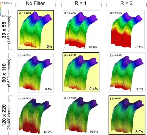
As shown in Fig. 7, applying Laplacian smoothing directly

to the evolved design has the effect of over-smoothing the

evolved features, and altering mechanical performance. Note

that while mechanical performance is worse, the shape and

size of the mesh elements are significantly improved and made

more regular. The central image in Fig. 7 shows the effect of

doubling the resolution from (30 x 55) elements to (60 x 110)

elements and applying a Laplacian smoothing filter with R =

1. Here we see a FE-mesh with significantly more uniform

elements and only 0.4% difference in simulated performance.

Similarly, we achieve a relatively small 3.7% error even as we

multiply the number of mesh elements by a factor of 16 times

(Fig. 8).

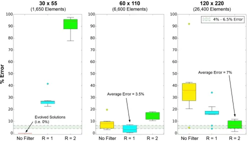
Figure 9 shows the results of testing all of our evolved

solutions at differing resolutions and with different filter

ranges. To compare our results we show our percentage error

in relation to the results of [13]. The authors show that their

solutions are

mesh independent

by altering the resolution of

their mesh between 1,650 and 6,600 elements and re-running

their gradient-based method to show that they converge on

equivalent solutions with about 4 – 6.5% error. In comparison,

we show an average error of 3.5% and 7% when increasing

resolution to

6,600

elements and

26,400

elements respectively.

By showing that the mechanical performance of our

evolved designs (Fig 5A) can be replicated using significantly

finer and more regular meshes (Fig 7-9) and - importantly -

using reliable C3D20R elements, we show that our method of

evolving surface-mapped CPPNs is not exploiting mesh

irregularities to produce deceptive results, and is indeed

improving on state-of-the-art gradient-based methods for

shape optimization. Specifically, we show that our method can

consistently discover mechanical designs that are better than

existing state-of-the-art methods [13].

IV.

SCALABILITY

EXPERIMENT

A.

Modifications to Methods

To test the scalability of our method, we explore eight

different parameterizations of the previous benchmark

problem (Fig. 2), and use two different surface

transformations. Firstly, we evolve designs with a uniform

shell thickness. Secondly, we evolve designs where shell

thickness is allowed to vary (locally) across the surface.

To build designs with

uniform

shell thickness, we use a

CPPN (as before) with three inputs, and one output (see Fig

1). To build designs with

variable

shell thickness, we use the

same CPPN method, but add an extra output,

T,

to control

shell thickness

. As shown in Figure 10,

Z

_{continues to define}

a surface extrusion relative to the surface normal, but now

T

defines the thickness of the shell across the surface. Here, T

defines the thickness of the shell at each (u,v) coordinate on

the NURBS substrate by locally extruding the shell in the

opposite direction of the surface normal, ensuring that the

minimum shell thickness at any point is 0.01mm and the

maximum is 1.0mm (Fig 10). The solution is then meshed and

subjected to FEA as the uniform shell. Note that a key

difference between the

uniform

and

variable

shell designs is

the number of degrees-of-freedom.

1)

Modifications to the Benchmark Setup

We add additional

degrees of freedom

(DoF) to the original

benchmark problem in order to demonstrate that, unlike

similar methods [4], [15], [17], the problem does not become

more difficult to solve as more DoF are added to the system.

To demonstrate this scalable behavior, we increase the

dimensionality of the problem in two specific ways, and test

eight different parameterizations of the benchmark problem.

Firstly, we vary the

discretization

of the FE-mesh. Our base

experiment used a fixed mesh resolution of 30 x 55 elements

(i.e. 1736 different DoF). In this paper we test four different

mesh resolutions: 6 x 12 elements (91 DoF), 12 x 24 elements

(325 DoF), 24 x 48 elements (1225 DoF), and 48 x 96

elements (4753 DoF). Here each

uniform

shell has a fixed

thickness of 0.3mm.

Secondly, we allow solutions to vary their discretization

and

shell thicknesses across the surface domain, subject to a

maximum volume constraint. Here the local shell thickness is

a continuous value between 0.01mm and 1.0mm. If the

volume of the final shell solution,

sV

, is greater than a

maximum volume,

mV

, the CPPN is re-queried and the

thickness,

T,

of each point is scaled linearly to meet

mV

.

We calculate the volume of each shell solution by taking

each finite element block (as shown in Fig 10), and splitting it

into twelve irregular tetrahedrons. Each tetrahedron is defined

by six edges:

a, b, c, A, B, C

, where the pairs (

a,A

), (

b,B

), and

(

c,C

) are opposite edges that do not share common vertices

(Fig. 11).

Figure 11. Irregular tetrahedron defined by six edges: a,b,c,A,B,C. The volume of each finite element block, as shown by the dotted bounding box, is calculated by summing the volume of 12 irregular tetrahedrons.

We calculate the volume of each tetrahedron,

tV

, as:

!"

=

(

4

!

!

_!

_!

₋

_!

_!

₋

_!

_!

_!

₋

_!

_!

_!

₊

_!

_!

_′

_!

_′

_!

_′

₎

!

12

Where:

!

₌

_!

_!

_+!

_!

₋

_!

_!

!

₌

_!

_!

_+!

_!

₋

_!

_!

We then calculate the volume of each shell by summing over

all tetrahedrons:

!"

=

!"

!!!

!

!!!

!!!!!!!!!!!!!!!!!!!!!!!!!!!!!!!!!!!!!!!!!!!!!!!!!!!!!!!!!!!!!!!!!!!!!!!!!!!

(

6)

where:

tVij is the volume of the

jth tetrahedron within the ith

finite element in a collection of N FE blocks.

To constrain sV of each shell to mV, we re-query the CPPN

and linearly scale the shell thickness, T, to meet mV using:

!

(

!

!"

!!!

,

!",

!")

!!!

Where:

!

!

∈

[0.01

∶

1]

!

!,

!",

!"

=

!

!,!!!!!!!!!!!!!!!!!!!!!!!!!!!!!!!!!!!!!!!!"!!"

_!!

_×

_!

₁

₋

_!

_!"

≤

!"!

!"

,!!!!!!"!!"!

>

!"

!!!!!!!!!

(

7)

where: Tuv is the local shell thickness generated by querying

the CPPN at point (u,v) on the NURBS surface, and Ut and Vt

are the total number of points on the NURBS surface in the u,

and v dimensions respectfully. Tuv can have a minimum value

of 0.01 and a maximum value of 1.0. In these experiments we

set

mV to 130mm

. Notably, shells with uniform shell

thickness of 0.3mm have a volume that is between 124.2mm

and 141.9mm

_{(depending on how points are extruded to form}

structural beads).

The important consequence of using variable shell thickness

is that it

doubles the number of DoF in each parameterization

of the benchmark problem. This creates eight different

parameterizations with increasing DoF:

91 and

182 (uniform

and variable shell thickness of discretization: 6 x 12), 325 and

650 (12 x 24), 1225 and

2450 (24 x 48), and 4753 and

9506

(48 x 96). These eight parameterizations allow us to test how

our surface-mapped CPPN approach performs across a range

of different scales.

As in our base experiment, we perform our finite element

calculations using the open-source solver

CalculiX, but this

time we use

C3D8 elements. Our base experiment used

C3D20R elements, which are robust and reliable FE brick

elements, in order to compare our solutions with a

state-of-the-art gradient-based approach [13]. C3D20R elements more

accurately simulate physical behavior, but the trade-off for

fine-grained analysis is increased computation time [45]. In

this experiment we use C3D8 elements, which are less

accurate, but much faster to simulate and therefore allow us to

explore the scalability of our approach in a reasonable

timeframe.

2)

Modifications to the NEAT Setup

We perform 20 independent runs of each of our 8

parameterizations, each run using a population of 100

solutions, evolved for 200 generations. All other details of the

NEAT setup and fitness function are the same as in the base

experiment.

Since we use different finite element bricks in this

benchmark setup, our results are not directly comparable to

solutions found in the base experiment. Consequently, our

decision to increase the number of runs and generations is due

to a desire to exploit the reduced runtimes of our simulations

(when using D3D8 elements) in order to provide a better

picture of

average convergence behavior across different

parameterizations of the benchmark problem.

A.

Results

We now present the results from eight different

parameterizations of the benchmark problem. Our focus is on

how designs converge as the benchmark problem increases in

scale. Our results show that, in contrast to traditional shape

optimization techniques, the benchmark problem

does not

become more difficult to solve as we increase the number of

degrees of freedom. Indeed, our results show that the

benchmark problem actually becomes

easier to solve with

higher resolution parameterizations.

We first test solutions with uniform thickness and varying

mesh resolution. Figure 12 shows the mean convergence of

the best solution in each population over 20 runs of the model.

As shown, the lowest resolution FE-mesh (i.e. 6 x 12

elements) converges to a displacement, |d|, of 0.073mm after

200 generations. We then see that for each successive increase

in scale, i.e. 12 x 24 elements, followed by 24 x 48 elements,

we converge to better solutions, and this trend continues as we

reach our highest resolution of 48 x 96 elements (4753 DoF),

which achieved an average |d| of 0.041mm.

Secondly, we test solutions with variable thickness and

varying mesh resolution. Figure 13 shows the mean

convergence of the best solution in each population over 20

runs. In a similar fashion to Figure 12, we see that higher

resolution FE-meshes converge to solutions with mechanically

superior performance (i.e. less displacement at the loaded

node). On first sight, this finding is perhaps not completely

surprising, as it is well-known that designs defined by more

degrees of freedom can often discover better solutions, due to

the increased opportunity for fine-tuning [21]. However, the

key point is that this ability typically comes at a cost of many

more evaluations and thus increased computational expense.

Indeed, designs with low resolution FE-meshes typically

converge quickly to sub-optimal solutions, whereas whilst

higher resolution FE-meshes can often find superior solutions,

they require many more evaluations to converge [9], [10].

Figures 12 and 13 illustrate that solutions evolved with

surface-mapped CPPNs are

not subject to this behavior. In

fact, we find that solutions controlled by more optimization

variables discover superior solutions in fewer evaluations.

parameterizations with both uniform and variable shell

thicknesses converge to the threshold of 0.0609mm in fewer

generations as more DoF are added to the solution. The

significance of this plot is that traditional shape optimization

methods produce the

inverse

effect – that is, as DoF increase,

so do the number of generations required to converge [9],

[21].

It is important to note that, in these experiments, higher

resolution parameterizations take fewer

evaluations

to

converge, yet do take more

time

to solve than lower-resolution

designs, due to the increased computational expense of the

FEA. This might initially appear to be an obvious limitation of

our approach. However, in practice, approaches which employ

strategies to reduce the dimensionality of the problem in order

to improve speed of convergence do not change the resolution

of the FEA mesh, but simply change the number of control

points that define DoF in the model [2], [4], [17], [18]-[21].

Consequently, our finding that parameterizations with more

DoF can discover superior solutions in fewer evaluations is

potentially significant for shape optimization.

Next, we compare how uniform and variable shell solutions

with identical mesh resolutions converge (Fig 15). We observe

that more DoF lead to better solutions (i.e. less displacement)

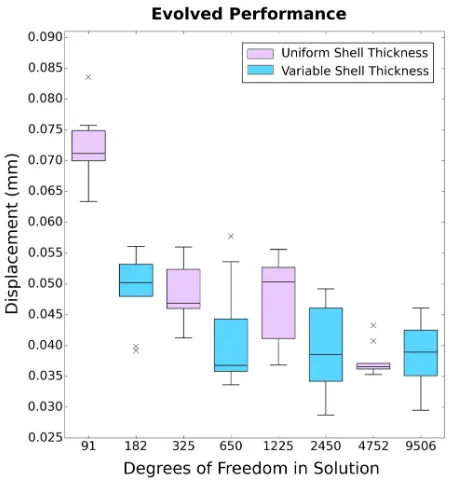
and faster convergence. Finally, Figure 16 shows the spread of

mechanical performance achieved across the eight different

parameterizations. This plot emphasizes our key finding, that

evolving surface-mapped CPPNs for shape optimization does

not become more difficult as more degrees of freedom are

added to the system. In contrast, we find that problems defined

by more DoF are consistently easier to solve and also

converge to superior solutions in fewer evaluations. For raw

convergence data collected from both experiments see:

https://dx.doi.org/10.6084/m9.figshare.3795888.v1.

These results, in parallel with the findings from our base

experiment, suggest significant potential for tackling complex

and large-scale shape optimization problems using

surface-mapped CPPNs.

V.

DISCUSSION

Our results demonstrate that surface-mapped CPPNs offer

practical improvements over state-of-the-art methods to shape

optimization. In this section we discuss (A) the advantages of

our approach in terms of the superior physical properties of

solutions; (B) the ability to scale up and solve design problems

with many degrees of freedom, and (C) exciting opportunities

for further exploration.

A.

Advantages Relating to Physical Performance

A significant feature of our method is that it does not

explicitly

define sensitivity filters. As evidenced by [13],

[41]-[44], different filter sizes constrain state-of-the-art

gradient-based methods to converge to specific local optima.

Consequently,

filter size

becomes an important design variable

that designers must experiment with to access different

solutions within the search space. But once the filter size is

set, it is

uniformly

applied to the mesh to smooth the design.

We claim that a key limitation of these state-of-the-art

approaches is that a

combination

of different filter sizes,

applied simultaneously across the design may conceivably

produce even better solutions than existing uniform filters.

This insight is the key to understanding

why

our

surface-mapped CPPNs improve on state-of-the-art methods.

Specifically, our approach uses CPPNs to paint functional

patterns across NURBS geometry to create coordinated mesh

transformations. Recall that the CPPN-generated patterns

exhibit useful features such as geometric regularities with

repeating motifs; symmetries and even imperfect symmetries;

and thus the capacity to create both smooth gradations and

more abrupt angular transitions between parts of the design.

This means that our encoding can

implicitly

control

smoothness

of geometric features during evolution, and,

critically, does so in a non-uniform manner that is not limited

in the same way as existing state-of-the-art gradient-based

methods.

A common criticism of

gradient-free

methods for shape

and structural optimization is that is that they cannot

guarantee

that the solutions converge to the global optimum.

This remains true with our approach. However as we have

discussed, in state-of-the-art shape optimization methods,

parameterization decisions involved in setting up sensitivity

filters actively define which “optimum” is discoverable.

Consequently, while our model cannot

guarantee

convergence

to an optimal solution, we seem better able to approximate the

true

global optima than state-of-the-art methods, and in doing

so, can discover solutions that have superior performance on

highly non-convex, real-world problems.

A.

Advantages Relating to Scalability

The results of our scalability experiment suggest that

surface-mapped CPPNs enable a powerful and

scalable

approach to shape optimization. Critically, our choice of

FE-mesh resolutions (6x12), (12x24), (24x48), (48x96) allow us

to test our benchmark problem at a variety of significantly

different scales, ranging from 91 to 9506 degrees of freedom.

This increase in scale is

substantial

compared to related

studies [2], [4], [9], [10], [17], [21], and also

significantly

exceeds

the 1,000 DoF threshold which is known to be

currently challenging for gradient-free methods due to the

need to individually parameterize and manipulate each DoF

[12]. However, we consistently discover superior solutions, in

fewer evaluations, when using parameterizations with more

degrees of freedom.

Figure 12. Convergence of uniform shell solutions with different DoF over 200 generations. Mean convergence,and variation of the best solution in each population across 20 runs are shown. Solutions defined by more DoF converge to better performing designs.

Figure 14. Convergence behavior of different parameterizations. Mean number of generations required to hit the threshold over 20 runs of the model is shown for each parameterization. Range of maximum and minimum generations required to converge to the threshold is also shown. Solutions with uniform shell thickness are plotted in red, and variable shell thickness in blue.

Critically, the shell designs with variable thickness do

not

use more material than those with uniform thickness (in fact,

in some cases they use less); rather, they are afforded the

capacity to

control where material is distributed whilst

defining how geometry is transformed. This type of

parameterization would traditionally be fraught with

scalability problems, especially when using EAs, yet our

surface-mapped

CPPNs

easily

coordinate

geometric

transformations to find good solutions.

Another useful property of our approach is that it is

conceptually relatively simple, and therefore (unlike adaptive

parameterizations) does not require specialist knowledge to

Figure 13. Convergence of variable shell solutions with different DoF over 200 generations. Mean convergence and variation,of the best solution in each population across 20 runs are shown. Solutions defined by more DoF converge to better performing designs.

Figure 16. Spread of best evolved solutions from all 20 runs, over 200 generations each time, using different parameterizations. As the number of DoF increases, better solutions (i.e. those showing less displacement at the loaded node) are discovered more regularly.

tune newly introduced problem specific parameters. In terms

of commercial application and use in industry, we suggest that

this is a major advantage. Future work will explore this

further.

shape optimization methods ignore this fact, instead choosing

to treat designs as collections of points, which are individually

parameterized, manipulated and then post-processed to

achieve smooth transitions and coordinated transformations.

By evolving surface-mapped CPPNs, we completely

re-frame the problem, and in doing so make high-resolution

geometric problems just as easy to solve as low-resolution

geometric problems. That is, instead of conceptualizing shape

optimization as a high-dimensional combinatorial optimization

problem, where the exact value of each parameter is sought,

our approach uses CPPNs to discover underlying geometric

and spatial relationships that are often (if not always) present

in these types of problems.

Critically, previous work relating to CPPN-based methods

of generating 3-D objects has also demonstrated this ability to

exploit free compositional information to create scale free

geometric transformations. However, by mapping the spatial

domain to specific surfaces – rather than using Cartesian

volumes – we are able to exploit free compositional

information relating to predefined geometries, while

simultaneously enforcing much-needed constraints on

engineering design problems.

In this paper we show that our approach is conceptually

easier to use than similar methods (i.e. adaptive

parameterizations), can produce superior mechanical solutions

compared to state-of-the-art gradient-based approaches on a

well-known benchmark problem, exploit the core benefits of

evolutionary methods in terms of addressing complex

multi-modal problem domains, and - perhaps most importantly -

operate well at large scales.

B.

Opportunities for Further Work

We now discuss several key benefits and opportunities for

progress in this area, as well as ongoing challenges that

require further work.

Advanced digital fabrication technologies (e.g. additive

manufacturing) are transforming construction. Not only do

these technologies offer vast geometric freedom to designs,

but also they allow us to combine

different materials within

single objects, and thereby construct complex composites with

bespoke physical properties and behaviors. These technologies

are opening up exciting possibilities for large-scale shell

structures in design and engineering domains [2], bio-inspired

composites [3], resilient high-performance shell designs [4],

next-generation robotics [31], exotic compliant mechanisms

and morphing structures [47], [48]. Evolutionary approaches,

such as surface-mapped CPPNs, that can deal with large

numbers of design variables and approximate optimal designs,

will offer significant benefits for exploiting these new

fabrication technologies by exploring highly non-convex and

disjoint search spaces in response to ill-defined and

multi-objective goals.

We conclude by outlining three areas for future research

that we think will be valuable in leveraging surface-mapped

CPPNs to advance engineering design.

Firstly, an ongoing challenge with our current setup is that it

is computationally expensive. That is, while our model

requires roughly the same number of

generations as

optimization steps required by [13] (i.e. to test all three filter

sizes), in order to discover superior solutions each generation

requires an additional 99 FEA evaluation calls, due to the need

to simulate populations of solutions. Consequently our

simulation time is about 100 times that of [13]. For example,

our base experiment, with 1,736 degrees of freedom, requires

about 17 hours run time to process 160 generations, which is

impractical for use within industry. However, we are currently

running our model on a single PC. Further work is required to

utilize cloud-based systems and evaluate individual solutions

from each generation in parallel. This would drastically reduce

the time required to solve design problems, make our method

much more suitable for commercial application, and render it

potentially comparable to gradient-based methods in terms of

time required to generate solutions.

Secondly, as we demonstrate in our base experiment, in

order to increase the resolution of evolved surface-mapped

CPPNs and produce similar solutions, it is necessary to

employ strategies that prevent under-smoothing and

over-smoothing (Fig 6). In this paper we demonstrate a simple

Laplacian smoothing operator in order to demonstrate that our

solutions are mesh independent. However, further work is

needed in this area to ensure that surface-mapped CPPNs can

be reliably recreated at any resolution without further

evolution. Additionally, while we show that surface-mapped

CPPNs eliminate the need for adaptive parameterizations on

large-scale problems, we suggest that there may be cases

where designs benefit from mesh solutions that feature

non-uniform discretization, or which perhaps feature adaptive

mesh strategies [49]. Specifically, there may be times when it

is easier to produce high-performance solutions with

FE-meshes, which are subdivided and discretized differently.

Notably, ES-HyperNEAT approaches [50] have proven useful

in other domains, and may provide useful insights for further

research in this area. Additionally, alternative methods of

exploiting CPPN outputs may enable high-performance

surface conformed truss and lattice structures [36], which may

be advantageous in specific problem domains.

Finally, this paper demonstrates shape optimization on one

benchmark problem only. To progress this proof-of-concept

study, further work is needed to test this approach on a variety

of different benchmark problems. Notably, the real benefit of

using EAs, rather than state-of-the-art gradient-based methods,

is that they can be applied to non-trivial design problems that

are characterized by deceptive search spaces, for example,

exotic compliant mechanisms, multi-material composites and

shape changing structures. Further work will explore material

maps as a method of addressing these sorts of

non-trivial

design problems, and fully exploit the benefits of evolutionary

methods to advance engineering design.

REFERENCES

[1] K. U. Bletzinger, M. Firl, J. Linhard, and R. Wüchner. "Optimal shapes of mechanically motivated surfaces." Computer methods in applied mechanics and engineering, vol. 199, no. 5, 2010, pp. 324-333. [2] S. Adriaenssens, P. Block, D. Veenendaal and C. Williams. Shell

structures for architecture: form finding and optimization. Routledge, 2014.