Eco efficiency analysis in generalized IO models: Methods and examples

Munich Personal RePEc Archive

Eco-efficiency analysis in generalized IO

models: Methods and examples

Gurgul, Henryk and Lach, Łukasz

AGH University of Science and Technology in Cracow, Poland

1 January 2019

Online at

https://mpra.ub.uni-muenchen.de/96604/

E

co-efficiency

analysis

in generalized IO models:

Methods and examples

Henryk Gurgul

(corresponding author)

Department of Applications of Mathematics in Economics, Faculty of Management, AGH University of Science and Technology, Gramatyka 10 st., 30-067 Cracow, Poland

tel.: +48 012 6174310, fax: +48 012 6367005, e-mail: [email protected]

Łukasz Lach

Department of Applications of Mathematics in Economics, Faculty of Management, AGH University of Science and Technology, Gramatyka 10 st., 30-067 Cracow, Poland

tel.: +48 012 6174218, fax: +48 012 6367005, e-mail: [email protected]

Abstract

Performance assessment in the presence of undesirable outputs, such as pollutant emissions, is

usually modelled within the framework of data envelopment analysis (DEA). In this paper we

propose a new approach to measuring eco-efficiency in generalized input-output (gIO) models

which may be used as a supplementary method to traditional DEA. Unlike DEA this approach

takes into account detailed data on intersectoral flows in supply- and demand-driven gIO

models. We focus on cases of traditional and sector-size-adjusted measures of interindustry

linkages in gIO models and in each case we suggest respective indices of eco-efficiency and

prove their usefulness in policymaking.

In order to illustrate possible applications of the new approach we conduct an empirical

analysis aimed at identifying the eco-efficient sectors based on the 1995 and 2009 national

input-output tables and environmental accounts for Poland which are provided by the World

Input Output Data (WIOD) database.

Keywords: generalized input-output models, intersectoral linkages, eco-efficiency, nonlinear

optimization.

1. Introduction

In recent years the issue of seeking ways to increase ‘eco-efficiency’, understood as a

management philosophy that aims at minimizing ecological damage while maximizing the

efficiency of a firm's production processes, has become a topic of considerable interest for

both researchers and politicians.1 Due to the increasing environmental burdens caused by

dramatic economic expansion, the issue of examining the ecological impact of economic

activities has turned out to be of special importance for developing and transition economies.2

From an operational perspective measuring the efficiency of economic activity with respect to

its environmental impact usually requires several steps. A crucial stage involves defining the

input and output variables used to build a model that could help to measure eco-efficiency. At

the next stage a set of specialized quantitative tools is used to establish the eco-efficiency

levels of the decision making units (DMUs) analysed, i.e. firms, managers, sectors of an

economy, etc. In this context data envelopment analysis (DEA)3 has grown into an

increasingly popular non-parametric tool used for performance evaluation. The main

advantage of DEA lies in the fact that it accomplishes the task of measuring performance

merely on the basis of the mathematical optimization approach without the need of subjective

weight assignment for inputs and outputs. In other words, DEA allows any number of DMUs

to be evaluated, with any number of inputs and outputs. The method requires the inputs and

outputs for each DMU to be specified and defines the efficiency of each DMU as the

weighted sum of outputs (i.e. the total output) divided by the weighted sum of inputs (i.e. total

input). Moreover, all measures of efficiency lie between 0% and 100% while the numerical

values of the weights are chosen in a way that maximises the efficiency of the particular

DMU. When it comes to the general advantages of DEA one should also mention the fact that

this approach allows a simultaneous analysis of outputs and inputs to be conducted and does

not require an a priori definition of the form of the efficiency frontier. On the other hand,

DEA ignores the effect of exogenous variables, ignores statistical errors and does not provide

practical recommendations on how to improve efficiency (Odeck and Alkadi, 2001; Avkiran

and Rowlands, 2008; Pestana and Peypoch, 2010; Jordá et al. 2012).

1

For recent reviews of eco-efficiency-related topics see Merli et al. (2018), Cheng et al. (2018) and Pham et al. (2019), among others.

2

See Muller and Yan (2018), Aklin et al. (2018), Kim and Park (2018), Kounetas (2018), Xing et al. (2018),

Andrić et al. (2019), Brunel and Johnson (2019) and Freire-González and Puig-Ventosa (2019), among others. 3

This concept was theorized and developed by Charnes et al. (1978).

In recent years, DEA has been mainly used in the context of measuring the eco-efficiency of

sectors that operate in an economy. An updated discussion about DEA models that involve

undesirable outputs, with an emphasis on economic-environmental context analysis may be

found in Scheel (2001) and Gomes and Lins (2008), among others. Despite all the

undisputable general advantages of this approach, one must underline that this concept fails to

fully satisfactorily address important features of economic systems in at least three particular

aspects.

First, as stressed by Dyckhoff and Allen (2001), the DEA approach must only be used when

the decision maker has no doubts about the technical relations between undesirable outputs

and certain inputs and outputs. At the same time, a DEA-based analysis of the eco-efficiency

of multiple (say, 𝑛𝑛) sectors operating in an economy is solely based on an analysis of aggregated sector-specific inputs and outputs (usually just a few) while crucial information on

intersectoral linkages (recall that for 𝑛𝑛 sectors one has 𝑛𝑛×𝑛𝑛 such interrelations) is not taken into account. As a consequence, this kind of detailed information is not used when

establishing the levels of sectoral eco-efficiency, although it is clear that the structure of

intersectoral input-output relations is an important factor that influences the levels of

aggregated sectoral pollutant emission and output. This oversimplification seems to

significantly reduce the possible range of policy recommendations as the conclusions

following from DEA-based analyses usually take the form of listing the sectors which should

reduce the amount of undesirable outputs. At the same time, no information is provided on

possible changes in the underlying input-output relations with the remaining sectors of an

economy that could also influence the levels of eco-efficiency.

Secondly, the DEA-based approach to measuring eco-efficiency does not allow supply- and

demand-driven production processes that take place in economic systems to be analysed

separately and in detail. The demand-driven effect occurs when production in sector 𝑗𝑗

expands which, in turn, implies that there will be higher demands from sector 𝑗𝑗 for goods and services produced by other sectors, which are required as intermediate inputs in sector 𝑗𝑗’s

production. If one assumes that there are no supply limitations, the latter implies that other

industries will react to the increased intermediate demands originating from sector 𝑗𝑗 and will expand their own production. When the origin of an impact (shock) comes from a sector as a

purchaser of intermediate inputs, Leontief’s demand-driven input-output model is used in

order to quantify its consequences on the entire economy, as this model fully captures the

demand-side impact and sectoral interlinkages (Temurshoev, 2016). Alternatively, if sector 𝑗𝑗

experiences expansion of output, the latter implies that increased amounts of products of

sector 𝑗𝑗 become available on the market, and, in particular, this surplus output could be used as intermediate inputs in production in other sectors of the economy. In this case, supplies

from sector 𝑗𝑗 (which plays the role of a seller of intermediate goods) for all the industries that

use products or services produced by sector 𝑗𝑗 in their production will increase. In such a context Ghosh’s supply-driven input-output model is used in order to quantify its influences

on the entire economy as this model fully captures the supply-side impact and sectoral

interlinkages.

Finally, as underlined by Tarancón et al. (2008) and Gurgul and Lach (2018c), in practical

applications one may face complex scenarios in which coefficients and benchmark variables

are subjected to a set of restrictions, or even a group of benchmark variables. In such cases,

the relevance of DEA-based measures of efficiency is not only determined by the elasticity of

the benchmark variable, but also by any type of limitations on free changes in the

coefficients.4 It must be underlined that although the DEA approach is doubtlessly a useful

tool for verifying performance, a purely mathematical approach to measuring efficiency may

not be able to fully satisfactorily take into account many economic mechanisms like

production technologies (especially the question of what is technically feasible when

changing input coefficients), competitive advantages, international trade relations and the

structure of global value chains. One should consider all these issues when interpreting

DEA-based results, which unfortunately was not always the case in the majority of previous

empirical studies.

Taking into account the three general problems listed above, in this paper we propose a new

approach to measuring eco-efficiency in generalized input-output (gIO) models. This method

is not intended to replace DEA as neither approach can be straightforwardly considered a

substitute for the other, rather they can be considered complementary methods. The approach

proposed in this paper builds upon a theory of intersectoral linkages and thus it looks at

economic processes from a perspective other than that of DEA-based models. The latter

makes the approach presented in this paper a supplementary proposal to the mainstream

approach. In contrast to DEA we suggest that detailed data on intersectoral flows should be

taken into account, which are available in demand- and supply-oriented gIO models. We

focus on cases of traditional and sector-size-adjusted measures of interindustry linkages in

4

Such restrictions could be budgetary, political, or technological (for instance, the balance between certain inputs) in nature (Gurgul and Lach, 2018c).

gIO models and in each case we propose respective indices of eco-efficiency and prove their

general usefulness in policymaking. In order to illustrate possible applications of the new

approach, the empirical analysis aimed at identifying the eco-efficient sectors is based on the

1995 and 2009 national input-output tables and environmental accounts for Poland, which are

provided by the WIOD database. Importantly, unlike previous studies that focus on

intersectoral flows and output-oriented key sector analyses in post-communist CEE

economies, we avoid the negative effects of double-counting by focusing on two particular

fundamental policy target variables – income per gross output and CO2 emissions per gross

output. To the best of our knowledge, both the theoretical and empirical parts of our paper are

novel proposals in the economic literature.

The structure of this paper is as follows. Section 2 contains a brief overview of the literature

on measuring eco-efficiency (also within the framework of input-output models) with

particular attention paid to previous empirical analyses conducted for Poland. In Section 3 the

outline of a new methodology for measuring eco-efficiency in supply- and demand-driven

gIO models is described. Section 4 presents the dataset and the main results of an illustrative

empirical example conducted for the Polish economy. Finally, in Section 5 we summarize the

major findings and suggest some directions for future research.

2. Literature review

There is a long list of studies particularly aimed at presenting the state of the art in DEA

models in the presence of undesirable outputs.5 One of the most comprehensive reviews of the

theoretical models and methods of DEA is the handbook edited by Zhu (2015). As the editor

is one of the most prominent researchers in the field and the authors of particular chapters are

major contributors to DEA theory, the book may be treated as a source of the current state of

the art in the theory of DEA research. The range of topics covers distance functions and their

value duals, cross-efficiency measures in DEA, integer DEA, weight restrictions and

production trade-offs, facet analysis in DEA, scale elasticity, benchmarking and

context-dependent DEA, fuzzy DEA, non-homogenous units, partial input-output relations, super

efficiency, treatment of undesirable measures, translation invariance, stochastic nonparametric

envelopment of data, and global frontier index. In a subsequent work Zhu (2016) provides an

5

Comp. Färe et al. (1989, 2000), Yaisawarng and Klein (1994), Lovell et al. (1995), Färe and Grosskopf (2003, 2004), Thanassoulis (1995), Rheinhard et al. (1999, 2000), Scheel (2001), Hailu and Veeman (2001), Zofío and

Prieto (2001), Dyckhoff and Allen (2001), Sun (2002), Seiford and Zhu (2002), Korhonen and Luptáčik (2003), Gomes et al. (2003), Gomes and Lins (2008) and more recently Tajbakhsh and Hassini (2018), Sueyoshi and Wang (2018), Allevi et al. (2018), Wu et al. (2018), Ma et al. (2018), Wei et al. (2019), and Galindro et al. (2019), among others.

extensive compilation of state-of-the-art empirical studies and applications for DEA. It

includes a collection of 18 chapters written by world DEA experts.6

Given the quality of existing comprehensive reviews of theoretical variants of DEA along

with reviews of their practical implementations, including the two excellent joint publications

edited by Zhu (2015, 2016) mentioned above, in subsequent parts of this section we will focus

solely on selected papers that form the backdrop to the outline of the new methodology

presented in Section 3.

2.1.General approaches to modelling undesirable outputs in a DEA context

As the field of uses of DEA has grown progressively, one distinctive research current has

focused on employing this technique to address the environmental consequences of

production processes. Nowadays DEA-based models not only handle conventional outputs

and inputs, but also allow bad or environmentally undesirable outputs, i.e., waste and

polluting effluents obtained as by-products of commercial outputs and inputs, to be included

in an analysis (Picazo-Tadeoa et al., 2011)

.

Dyckhoff and Allen (2001) and Gomes and Lins (2008) discuss the advantages and

disadvantages of three main approaches to modelling undesirable outputs in a DEA context

,

which differ slightly in terms of the frequency of uses in empirical studies. The first one uses

the reciprocal of the undesirable output as DEA output, that is, the numerical variable

representing the undesirable output is first inverted and then modelled as a usual desirable

output. This approach is employed, for example, by Lovell et al. (1995) and is called

‘reciprocal multiplicative’ (Golany and Roll, 1989; Scheel, 2001). The second method

(Rheinhard et al., 1999) considers DEA to be a multi-criteria approach in which the

6

The range of empirical topics analysed covers the performance of CEOs of U.S. banks and thrifts, the network operational structure of transportation organizations and the relative network data envelopment analysis model, examples of using different types of DEA models to compute total-factor energy efficiency scores with an application to energy efficiency, the exploration of the impact of incorporating customers' willingness to pay for service quality in benchmarking models on the cost efficiency of distribution networks, a brief review of previous applications of DEA in the professional baseball industry, a DEA-based examination of the efficiency and productivity of U.S. property-liability insurers, a two-stage network DEA model that decomposes the overall efficiency of a DMU into two components, a review of the literature of DEA models for the performance assessment of mutual funds, a discussion on the management strategies formulation of the international tourist hotel industry in Taiwan, a novel use of the two-stage network DEA to evaluate sustainable product design performances, a description of the limitations of some DEA environmental efficiency models, reviews of the use of DEA in secondary and tertiary education, a review of measures of the relative performance of New York State school districts in the academic year 2011-2012, a detailed description of uses for DEA in marketing, a description of the decomposition of a new total factor productivity index that satisfies all economically-relevant axioms from index theory with an application to U.S. agriculture and a unique study that conducts a DEA research front analysis, using a network clustering method to group the DEA literature over the period 2000 to 2014.

undesirable output is modelled as an input. In this case, both the CCR and BCC7 variants of

the DEA models can be used, depending on the operational scale of the DMUs. As mentioned

by Scheel (2001), when considering undesirable outputs to be inputs, one creates the same set

of production variants as in the case of considering the undesirable outputs to be desirable

ones by using a reciprocal additive transformation. The third approach is based on values

translation (Ali and Seiford, 1990), which technically requires the reciprocal additive

transformation of the undesirable output to be increased by adding a positive scalar big

enough to ensure that the modified values are positive for each DMU.8

2.2. IO-related modifications

The initial DEA-based approach to modelling the undesirable approach has been modified in

many ways. A few modifications that turned out to be especially influential for empirical

analysis can be found in works by Färe et al. (1996) and Kuosmanen (2005), who formulate

an alternative approach to modelling undesirable emissions as outputs, assuming that these

undesirable outputs are ‘weakly disposable’, which generally means that it is possible to abate

emissions by decreasing the level of production activity. Korhonen and Luptáčik (2004) also

describe several alternative models for assessing eco-efficiency and test their ability to

provide similar efficiency scores for a sample of European power plants. They expound two

different approaches used to incorporate eco-efficiency in DEA models. The first requires

separate evaluations of technical and ecological efficiency to be computed via a DEA-based

approach and then these efficiency figures should be used as output variables in a new DEA

model. The second model consists in building up a ratio which simultaneously takes into

account both desirable and undesirable outputs, and leads to a wide variety of alternative

models, depending on how the undesirable outputs are treated.

From the perspective of the goal of this paper special attention must be paid to those studies

that connect DEA-based concepts of measuring the eco-efficiency of economies with methods

of exploring detailed information on interindustry relations contained in input-output data. At

this point it seems necessary to refer to the pioneering works of Luptáčik and Böhm (2010)

and Mahlberg and Luptáčik (2014). Both these studies are concerned with efficiency analysis

applied to a single economy represented by Leontief’s input-output model extended by

primary factor constraints. This methodological approach requires an efficiency frontier to be

7

These abbreviations refer to the names of the creators of the models, i.e. Charnes, Cooper and Rhodes for the CCR (Charnes et al., 1978) and Banker, Charnes and Cooper for the BCC (Banker et al., 1984).

8

Gomes and Lins (2008) stress that this approach is only valid for BCC and additive DEA models (Charnes et al., 1985), since CCR is not translation invariant (Cooper et al., 2000).

generated on the basis of a multi-objective optimization model instead of having to use data

from different DMUs. The solutions to the multi-objective optimization problems define

efficient virtual DMUs and the efficiency of a given economy is next defined as the difference

between the potential of an economy and its actual performance and can be obtained as a

solution to a DEA model. At the second stage the approach is extended to Leontief’s

augmented model, including emissions of pollutants and abatement activities, which in turn

provides an IO-based tool for the analysis of eco-efficiency of an economy.

The most serious drawback of the proposals of Luptáčik and Böhm (2010) and Mahlberg and

Luptáčik (2014) is the lack of statistical data required to construct the augmented Leontief

model. The models of Luptáčik and Böhm (2010) and Mahlberg and Luptáčik (2014) require

data on the matrix of primary input coefficients for abatement activities. As these data are not

available from any data source they are approximated by the authors using the perpetual

inventory method based on the time series of gross fixed capital formation for environmental

protection. Although the perpetual inventory method is a popular tool used for approximating

the unknown matrices of parameters in augmented and dynamic IO models (comp. Gurgul

and Lach, 2016, 2018d, among others), its accuracy in practical uses is still a source of serious

concern among empirical IO practitioners.9

An alternative approach to traditional DEA-based efficiency analysis in input-output models

is proposed by Prieto and Zofío (2007). They undertake a network efficiency analysis within

an input-output model that allows them to assess potential technical efficiency gains by

comparing technologies corresponding to different economies. As a result they outline an

algorithm for optimizing primary input allocation, intermediate production and final demand

production by way of non-parametric DEA techniques. Moreover, this model optimizes the

underlying multi-stage technologies that the input-output system comprises, identifying best

practice economies. However, there are two crucial shortcomings of the approach of Prieto

and Zofío (2007). First, the final outcome of the algorithm proposed takes the form of a

matrix of optimal changes to be implemented in an original input matrix. However, as

emphasized by Tarancón et al. (2008) and Gurgul and Lach (2018c), proper modelling of

changes in IO coefficients should take into account budgetary, political, or technological

limitations to free changes in the coefficients examined. Secondly, even if each individual

9

Recently Gurgul and Lach (2019) went beyond the limitations of previous studies and instead of setting the crucial parameters of the dynamic endogenous input–output model with layers of techniques on an arbitrary basis they proposed a new optimization-based approach to approximating the elements of capital matrices (which are not available in statistical bureaus) on the basis of available historical data.

element of the matrix of optimal changes obtained lies at a reasonable (from an economic

point of view) interval one cannot say that the whole set of changes suggested may take place

in an economy at the same time (this type of general recommendation is the main policy

implication of this approach). Taking this issue into account seems to be a promising direction

for future extensions and generalizations of the approach.10

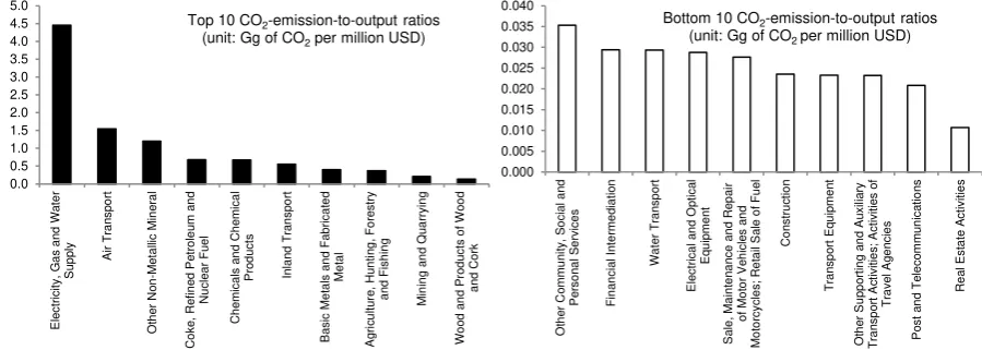
2.3.Measuring eco-efficiency in the Polish economy

There are several reasons for choosing Poland as a case study for the empirical part of this

paper, in which focus is placed on two particular fundamental policy target variables – income

per gross output and CO2 emissions per gross output. First, Poland has the sixth-highest GDP

(measured in PPP standards) in the EU and is an increasingly important player in the world

economy. At the same time Poland has the fifth-highest level of greenhouse gas emissions in

the EU. According to recent data published by WHO, 36 out of the 50 most polluted

European cities are located in Poland. As a consequence, particulate pollution from fossil fuel

combustion causes almost 50,000 deaths each year in Poland.

Secondly, in recent years Poland has not embraced tough emissions reductions targets, while

most European countries have implemented various environment-friendly policies.11 The lack

of enthusiasm for climate policy in Poland can be explained to a great extent by the strong

impact of trade union leaders in the coal industry on politicians. Since mining and burning

coal has a long tradition in Poland, many citizens (especially miners and their families living

in Śląskie province) cannot imagine their future without the existence of coal mines. In

addition, a significant number of politicians believe that coal mines in Poland are necessary to

provide an energy supply that will guarantee Poland’s independence from Russia in terms of

energy, Russia being the main supplier of natural gas and oil to Poland. However, since coal

has long been on a downward trajectory in Poland, as foreign countries with easily-accessible

coal and more modern mining technology have driven down global coal prices, Poland has

switched to importing millions of tons of coal per year. Ironically, most of this coal comes

from Russia.

10

Gurgul and Lach (2018c) propose a new algorithm for tracing value-added-redistribution-important coefficients (VARDI coefficients, in short) in a global IO model that deals with the issue of ranking the importance of individual coefficients belonging to an optimal solution, i.e. the set of VARDI coefficients. 11

For example, in 2015, Poland prevented the 28-member EU from ratifying the Kyoto Protocol on CO2 emissions as a bloc by voting for an amendment to the treaty. In 2016, Poland passed a law that hinders the development of wind energy (the new regulations included a requirement that turbines be located at a distance of at least 10 times the turbine’s height from any buildings or forest, and a requirement that allowed for extended shutdowns for inspections; moreover a fourfold increase in taxes on wind farms was authorized). In 2018, Poland’s climate negotiators officially admitted that pushing for stronger national pledges to reduce pollution is not one of the highest priorities of the authorities.

Taking all the these facts into account it seems obvious why in recent years one has noticed a

growing number of studies aimed at analysing eco-efficiency in the Polish economy that were

usually based on the use of some variants of the DEA approach.12 Rączka (2001) identifies

factors influencing the technical efficiency of heat plants in the Wielkopolska Region of

Poland. Technical efficiency scores were first obtained from a DEA model for a cross-section

sample of 41 heat plants. Next, a tobit model was used to explain the variability of the

efficiency index. Rączka (2001) showed that government intervention in the household

segment of the market decreased the efficiency of heat generation. At the same time coal

quality and capital utilization were found to increase the technical efficiency. Finally, the

results provided a basis to claim that public heat plants perform on average better than

municipal and industrial ones.

Czaplicka-Kolarz et al. (2015) suggest a new method for assessing the eco-efficiency of

mining production processes in hard coal mines in Poland, which enables the results of

evaluating both the environmental and economic aspects to be integrated. This method uses

the life cycle assessment (LCA) approach to assess the environmental efficiency and the

results of operating activities to assess economic efficiency. A comprehensive method for

assessing mining production processes is proposed as the key performance indicator in hard

coal mines in Poland to be used to support decision making in mining companies.

Masternak‐Janus and Rybaczewska‐Błażejowska (2017) examine the possibility of using the

concept of eco‐efficiency at a regional level to promote the sustainable transformation of the

regions of Poland. They decide to base their respective calculations on the input-oriented

CCR DEA method as this approach is highly capable of measuring regional eco‐efficiency.

The results of the study reveal that the provinces of Lubuskie, Mazowieckie, Śląskie,

Warmińsko‐Mazurskie, and Wielkopolskie are relatively eco‐efficient, whereas the remaining

regions use too many environmental resources in relation to the value of goods and services

produced. Six of the eleven eco‐inefficient regions in Poland have increasing returns to scale,

that is, the usage of natural resources connected with the negative impact upon the

environment is rising more slowly than the values of goods and services.

In a subsequent study Rybaczewska-Błażejowska and Masternak-Janus (2018) once again

focus on the case of Polish regions and the combined use of LCA and the input-oriented BCC

12

In general, in recent years one could notice that a broad set of energy-and-climate-related topics in economic

literature have been deeply analysed based on Polish data (comp. e.g. Dobrowolski et al. 2006; Boratyński, 2015;

Gurgul and Lach, 2011, 2016b; Lach, 2011, among others). However, given the scope of this paper, we will focus mainly on recent DEA-related empirical studies which used Polish energy economics data.

DEA model. The ultimate goal of this approach is to support the strategic decision-making

process. Firstly, it is shown that four of the sixteen Polish regions were found to be relatively

eco-efficient, with agriculture and services making the greatest contribution to GDP. The

study proves that the region with the most detrimental impact on the environment in all areas

of protection, i.e. Śląskie province, is also the most eco-inefficient one. Among the

fundamental sources of eco-inefficiency the authors list cumulative airborne emissions

(primarily CO2) and the excessive consumption of fuels, energy and heat in relation to the

value of the goods and services produced.

To summarize, the analysis of the current state of the art in the eco-efficiency literature

reveals an important fact. When it comes to the methodological details of the mainstream

approach to measuring the eco-efficiency of economies one can see that DEA-based tools

occupy a dominant position. This is also true in the case of studies that aim at examining the

eco-efficiency of Poland. Unlike the dominant approach, in this paper we propose a new

approach to measuring eco-efficiency in gIO models, which may be used as a supplementary

method to traditional DEA.

3. Methodology

The main advantage of the proposed method is the fact that it takes into account detailed data

on intersectoral flows in supply- and demand-oriented gIO models. Thus, in order to

formulate respective eco-efficiency indices and prove their usefulness in policymaking we

start this section with a brief overview of the most important measures of linkages which we

shall then use to construct efficiency indices. In general, our approach to measuring

eco-efficiency builds upon the fundamentals of so-called ‘key sector analysis’. In general, the

purpose of key sector analysis is to identify those sectors which have the greatest effects on

the rest of the economy (Gurgul and Lach, 2015).

3.1. Key sector measures - overview

The specific branch of literature that focuses solely on the analysis of sectoral input-output

(IO) linkages and key sectors occupies a central place in the field of input-output analysis. In

this context one should agree with Temurshoev (2016), who emphasizes that the analysis of

IO linkages provides all the necessary tools required to better understand the importance of

intersectoral interrelations in an economy. More precisely, such analyses may focus on

addressing and/or evaluating various economic development policies that target specific

industries. In particular, the direct and indirect strength of sectoral interdependencies can be

quantified, which sheds light on the significance of individual sectors in the functioning of the

entire economy (Temurshoev and Oosterhaven, 2014). Thus, it is not surprising that for many

years the identification of key sectors in an economy has been one of the most important

research topics in input–output analysis.13 In any economy the identification and classification

of its most influential branches can provide the basis for a taxonomy of the economy and can

contribute to a better understanding of growth and development problems.

As stressed by Miller and Blair (2009), in the framework of input-output models, the process

of production that takes place in a particular sector 𝑗𝑗 implies two kinds of economic effects on other sectors of the economy:

 Assume that sector 𝑗𝑗 increases its output. The latter implies that demands from sector 𝑗𝑗 (which acts as a purchaser) on those sectors whose goods are used as production

inputs in sector 𝑗𝑗 will increase. This direction of a causal relationship is typical for a usual demand-side input-output model. In the input-output literature, this kind of

interconnection between a particular sector and those (‘upstream’) sectors from which

the latter purchases inputs is referred to as a so-called ‘backward linkage’.

 Alternatively, an increase in output in sector 𝑗𝑗 implies that additional amounts of products from sector 𝑗𝑗 become available to be used as inputs to other sectors for their

own production. In other words, an increase in supplies from sector 𝑗𝑗 (acting as a seller) for the sectors that use the products of sector 𝑗𝑗 in their production processes

takes place. This in turn is the direction of causality in the usual supply-side IO model,

and the term ‘forward linkage’ is used to indicate this kind of interconnection between

a particular sector and those (‘downstream’) sectors to which it sells its output.

Following Temurshoev’s (2016) review of the literature on the methods of key sector

analysis, throughout this study two general types of measures of interindustry linkages will be

studied within the framework of gIO models. These measures are related to two general

concepts of measuring interindustry linkages: traditional mathematical measures of backward

and forward linkages, and sector-size-adjusted interindustry linkages.14

13

Since the release of the pioneering work of Hirschman (1958), the concept of the use of linkages in measuring interindustry relationships in an economy has attracted considerable attention among theoreticians and empiricists (Chenery and Watanabe, 1958; Hewings and Romanos, 1981; Hewings, 1982; Defourny and Thorbecke, 1984; Gurgul and Lach, 2016, 2018a, 2018b, 2018c, 2019; Zheng et al., 2018).

14

In the IO literature there are several main types of interindustry linkages (Lahr, 2001). However, as pointed out by Temurshoev (2016), all the main types of sector-size-independent linkage may be easily derived on the basis of traditional linkages. Similarly, from a mathematical point of view the main types of sector-size-adjusted linkage are also functions of traditional linkages. Thus, throughout this study we restrict our analysis to the two variants of linkage measures.

3.2. Traditional linkages

Before providing respective formulas for calculating traditional interindustry linkages let us

start by presenting some notational remarks which will make reading subsequent parts of the

study easier. Since the aim of the empirical part of this paper is to analyse the efficiency of

income generation with respect to the corresponding CO2 emission of sectors operating in

Polish economy, let us assume that the economy being studied consists of 𝑛𝑛 sectors. Next, let 𝜋𝜋𝑖𝑖𝐼𝐼𝐼𝐼𝐼𝐼,𝑡𝑡 stand for sector 𝑖𝑖′𝑠𝑠 direct coefficient indicating the generation of income per unit of

gross output and let 𝜋𝜋_𝑖𝑖𝐼𝐼𝐶𝐶_,𝑡𝑡2 _{denote sector} 𝑖𝑖′𝑠𝑠 _{direct coefficient of CO}

2 emissions per unit of

gross output, both given at time point 𝑡𝑡. Next, let 𝐱𝐱_𝑡𝑡= [𝑥𝑥_𝑖𝑖𝑡𝑡,𝑖𝑖= 1, … ,𝑛𝑛] stand for the 𝑛𝑛 −element vector of output, 𝐟𝐟_𝑡𝑡= [𝑓𝑓_𝑖𝑖𝑡𝑡,𝑖𝑖 = 1, … ,𝑛𝑛] stand for the 𝑛𝑛 −element vector of final demand, 𝐯𝐯_𝑡𝑡 = [𝑣𝑣_𝑖𝑖𝑡𝑡,𝑖𝑖= 1, … ,𝑛𝑛] stand for the row of sectoral value added, 𝐋𝐋_𝑡𝑡 = (𝐈𝐈 − 𝐀𝐀_𝑡𝑡)−1=

�𝑙𝑙𝑖𝑖𝑖𝑖𝑡𝑡,𝑖𝑖,𝑗𝑗= 1, … ,𝑛𝑛� denote 𝑛𝑛×𝑛𝑛 Leontief inverse and 𝐆𝐆𝑡𝑡 = (𝐈𝐈 − 𝐂𝐂𝑡𝑡)−1 =�𝑔𝑔𝑖𝑖𝑖𝑖𝑡𝑡,𝑖𝑖,𝑗𝑗 = 1, … ,𝑛𝑛�

stand for 𝑛𝑛×𝑛𝑛 Ghosh inverse, where 𝐀𝐀_𝑡𝑡= �𝑎𝑎_{𝑖𝑖𝑖𝑖}𝑡𝑡,𝑖𝑖,𝑗𝑗 = 1, … ,𝑛𝑛� and 𝐂𝐂_𝑡𝑡 =�𝑐𝑐_{𝑖𝑖𝑖𝑖}𝑡𝑡,𝑖𝑖,𝑗𝑗 = 1, … ,𝑛𝑛�

denote input and output matrices, respectively.15

In general, key sector measures were predominantly used in studies that focused on gross

output, especially in the early input-output research (Gurgul and Lach, 2015). However, the

output-oriented measures of intersectoral dependencies obtained in basic Leontief/Ghosh

models have a serious drawback. Namely, in order to be relevant to actual policymaking, key

sector measures should be defined in a way that could reflect not only the gross-output-related

processes but also the other main policy goals, including income generation, job creation, or

reduction of greenhouse gas emission (Oosterhaven, 1981; Lenzen, 2003; Garrett-Peltier,

2017). Moreover, gross output reflects double-counting as it includes both the sales of

intermediate and final products (thus, it is also often referred to as ’gross duplicated output’).

Therefore, in practical applications one uses generalized IO models to conduct policy-oriented

multiplier analysis (Gurgul and Lach, 2018a). Since the level of factor production/use in any

sector 𝑖𝑖 (henceforth we will denote this as 𝑒𝑒_𝑖𝑖𝑡𝑡) can be easily computed as 𝑒𝑒_𝑖𝑖𝑡𝑡= 𝜋𝜋_𝑖𝑖𝑡𝑡𝑥𝑥_𝑖𝑖𝑡𝑡, where 𝜋𝜋_𝑖𝑖𝑡𝑡

stands for analyzed policy goal variable,16 the so-called ‘generalized demand-driven IO

model’ may be defined using the following formula (Miller and Blair, 2009):

𝐞𝐞𝒕𝒕 =𝛑𝛑�𝒕𝒕𝐋𝐋𝒕𝒕𝐟𝐟𝒕𝒕, (1)

15

Following the usual notation in the IO literature, throughout this paper matrices are indicated by bold capitals, vectors by bold lowercases and scalars by italic capitals and lowercases. In this paper the symbols 𝐱𝐱� and 𝑑𝑑𝑖𝑖𝑎𝑎𝑔𝑔(𝐱𝐱)

will be used interchangeably to denote a diagonal matrix with elements of vector 𝐱𝐱on the main diagonal. 16

In the case of the empirical example analysed in this paper 𝜋𝜋_𝑖𝑖𝑡𝑡=𝜋𝜋_𝑖𝑖𝐼𝐼𝐼𝐼𝐼𝐼_,𝑡𝑡 or 𝜋𝜋_𝑖𝑖𝑡𝑡=𝜋𝜋_𝑖𝑖𝐼𝐼𝐶𝐶_,𝑡𝑡2.

where 𝐞𝐞_𝑡𝑡 = [𝑒𝑒_𝑖𝑖𝑡𝑡,𝑖𝑖= 1, … ,𝑛𝑛], and 𝛑𝛑�_𝑡𝑡 stands for a diagonal matrix with elements 𝜋𝜋_𝑖𝑖𝑡𝑡 on the

main diagonal. Similarly, one may define the so-called ‘generalized supply-driven IO model’,

which links sectoral primary inputs to factor production/use by means of the following

formula (Miller and Blair, 2009; Temurshoev, 2016):

𝐞𝐞′𝑡𝑡=𝐯𝐯𝑡𝑡𝐆𝐆𝑡𝑡𝛑𝛑�𝑡𝑡. (2)

As pointed out by Temurshoev (2016) and Gurgul and Lach (2018a), in input-output

linkage analysis it is now widely accepted and strongly advocated that any backward

linkage indicator, which measures the economy-wide degree of the complex (direct and

indirect) interrelatedness of sectors in their role as intermediate purchasers, should be

based on the demand-driven input-output model. Similarly, measuring the overall extent

of the complex interconnectedness of industries in their role as intermediate suppliers,

should be based on the supply-driven input-output model.17 Thus, forward linkage

indicators should be based on an application of Ghosh input-output model. Taking both

these facts into account, in later parts of this paper we will use the following definition of

traditional backward input-output linkage for sector 𝑖𝑖 and policy goal variable 𝛑𝛑_𝑡𝑡:

𝐵𝐵𝑖𝑖,𝑡𝑡(𝛑𝛑) =∑𝑛𝑛𝑘𝑘=1𝜋𝜋𝑘𝑘𝑡𝑡𝑙𝑙_{𝑘𝑘𝑖𝑖}𝑡𝑡 , (3)

and the following definition of traditional forward linkage:

𝐹𝐹𝑖𝑖,𝑡𝑡(𝛑𝛑) =∑𝑛𝑛𝑘𝑘=1𝑔𝑔_{𝑖𝑖𝑘𝑘}𝑡𝑡 𝜋𝜋𝑘𝑘𝑡𝑡. (4)

The backward input-output linkage defined in (3) reflects the demand-pull effects in an

economy. 𝐵𝐵_{𝑖𝑖,𝑡𝑡}(𝛑𝛑) measures the total (i.e. direct and indirect) intermediates’ purchase-related linkages/importance of sector 𝑖𝑖 which are associated with its unit final demand. In

other words, this indicator is a measure of the quantitative significance of the chains of

sector 𝑖𝑖’s demands for intermediate inputs from all sectors of the economy. The forward input-output linkage defined in (4) reflects the cost-push effects in the economy; i.e., it is

assumed that the input and output prices may change, but their quantities will remain fixed.

𝐹𝐹𝑖𝑖,𝑡𝑡(𝛑𝛑) refers to the total (i.e. direct and indirect) intermediates’ sales-related

linkages/importance of sector 𝑖𝑖 (in the sense of the quantitative significance of the chains of sector 𝑖𝑖’s supplies of its intermediate inputs to all sectors of the economy) which are

associated with its primary inputs equal to one unit.

17

From a historical point of view one should also mention ‘direct’ input-output linkages, which were defined as column sums of input matrix 𝐀𝐀_𝑡𝑡 (backward linkages; see e.g. Chenery and Watanabe (1958) for an early empirical application) and row sums of output matrix 𝐂𝐂_𝑡𝑡 (forward linkages). However, as stressed in Temurshoev (2016) these measures are nowadays rarely used in practical applications.

3.3. Sector-size-adjusted linkages

It should be stressed that the heterogeneity of industries in terms of their size should also be

explicitly taken into account in empirical applications, which is not always the case in the

existing key sector studies. Temurshoev (2016) and Gurgul and Lach (2018a) show that if the

effect of sector size is not corrected for, one would very often obtain the expected outcome

that big (small) industries have a big (small) impact on the whole economy, which will further

disregard the greater cost of stimulating a large industry. Therefore, in practical applications it

is also important to consider the total economy-wide impact of sectors per unit of their direct

size/contribution. For this purpose, along with the traditional input-output linkages their

sector-size-adjusted variants are also used in this study. This adjustment is simply based on

taking into account the relevant size or direct impact of the sectors:

𝐵𝐵�_𝑖𝑖,𝑡𝑡(𝛑𝛑) =

𝐵𝐵𝑖𝑖,𝑡𝑡(𝛑𝛑)

𝜋𝜋_𝑖𝑖𝑡𝑡 , (5)

𝐹𝐹�𝑖𝑖,𝑡𝑡(𝛑𝛑) =

𝐹𝐹_𝑖𝑖,𝑡𝑡(𝛑𝛑)

𝜋𝜋_𝑖𝑖𝑡𝑡 . (6)

The sector-size-adjusted linkage defined in (5) is a dimensionless indicator that expresses the

relevant traditional backward IO linkage of a particular sector per unit of its size given in

terms of the policy goal variable. From a supply-side perspective, one may analogously define

the sector-size-adjusted forward IO linkage using the formula (6). Like its traditional

counterpart, the sector-size-adjusted forward input-output linkage also reflects the cost-push

effects in the whole economy.

It is worth emphasizing that in comparison to the traditional linkages given in (3) and (4), the

sector-size-adjusted linkages in (5) and (6) treat all country-sectors similarly irrespective of

their size in generating the policy goal variable (Miller and Blair, 2009). Therefore, the

sector-size-adjusted IO linkages are more effective indicators of the indirect economy-wide impact

of the sectors relative to their own direct contribution. In this sense, sector-size-adjusted IO

linkages are somewhat superior to sector-size-independent measures as they are free of biases

resulting from the size of the sector (Temurshoev, 2016; Gurgul and Lach, 2018a).

A convenient way of interpreting the linkages in (3)-(6) is based on re-calculating their values

relative to the relevant economy-wide average. Henceforth, let ‖∙‖ denote the normalizing

operator which for the vector of nonnegative numbers 𝐱𝐱 = (𝑥𝑥_𝑖𝑖)_{𝑖𝑖=1,…,𝑛𝑛} is defined as follows:

‖𝐱𝐱‖= (‖𝑥𝑥_𝑖𝑖‖)_{𝑖𝑖=1,…,𝑛𝑛} = �_∑𝑛𝑛𝑥𝑥𝑖𝑖 𝑥𝑥𝑠𝑠 𝑛𝑛

𝑠𝑠=1 �_𝑖𝑖=1,…,𝑛𝑛

. ₍₇₎

Under such a notation the normalized linkages in (3)-(6) are simply defined as �𝐵𝐵_{𝑖𝑖,𝑡𝑡}(𝛑𝛑)�,

�𝐵𝐵�𝑖𝑖,𝑡𝑡(𝛑𝛑)�, �𝐹𝐹𝑖𝑖,𝑡𝑡(𝛑𝛑)� and �𝐹𝐹�𝑖𝑖,𝑡𝑡(𝛑𝛑)�, respectively. If the backward (forward) linkage of sector 𝑖𝑖

is greater than the economy-wide average of the corresponding backward (forward) linkages

of all sectors then the normalized backward (forward) linkage of this sector is greater than

unity.

3.4. Measuring eco-efficiency in generalized IO models

We suggest that eco-efficiency should be measured in gIO models in a way similar to the

general DEA-based approach, i.e. to define the eco-efficiency indicator as a ratio of output

effect to input stimulation. Since we distinguish between backward and forward linkages in an

economy, one should define separately the respective measures of the ‘backward

eco-efficiency’ and ‘forward eco-eco-efficiency’. In the case of the two-dimensional (i.e., single

output and single input) case, examined in the empirical part of this paper, we propose the

following formulas to define the linkage-based measures of the eco-efficiency of sector 𝑖𝑖 at

time point 𝑡𝑡:

𝐸𝐸𝐼𝐼𝐶𝐶𝐸𝐸𝐹𝐹𝐹𝐹_𝑖𝑖𝐵𝐵𝐵𝐵𝐼𝐼𝐵𝐵,𝑡𝑡 =

�𝐵𝐵𝐵𝐵𝐼𝐼𝐵𝐵_𝑖𝑖,𝑡𝑡(𝛑𝛑𝑂𝑂𝑂𝑂𝑂𝑂,𝑡𝑡)� �𝐵𝐵𝐵𝐵𝐼𝐼𝐵𝐵_𝑖𝑖,𝑡𝑡(𝛑𝛑𝐼𝐼𝐼𝐼

,𝑡𝑡_)�, (8)

𝐸𝐸𝐼𝐼𝐶𝐶𝐸𝐸𝐹𝐹𝐹𝐹_𝑖𝑖𝐹𝐹𝐶𝐶𝐹𝐹𝐹𝐹,𝑡𝑡 =

�𝐹𝐹𝐶𝐶𝐹𝐹𝐹𝐹_𝑖𝑖,𝑡𝑡(𝛑𝛑𝑂𝑂𝑂𝑂𝑂𝑂,𝑡𝑡)� �𝐹𝐹𝐶𝐶𝐹𝐹𝐹𝐹_𝑖𝑖,𝑡𝑡(𝛑𝛑𝐼𝐼𝐼𝐼,𝑡𝑡)�

, (9)

where:

• _{𝐸𝐸𝐼𝐼𝐶𝐶𝐸𝐸𝐹𝐹𝐹𝐹𝑖𝑖}𝐵𝐵𝐵𝐵𝐼𝐼𝐵𝐵_{,𝑡𝑡 (𝐸𝐸𝐼𝐼𝐶𝐶𝐸𝐸𝐹𝐹𝐹𝐹}

𝑖𝑖𝐹𝐹𝐶𝐶𝐹𝐹𝐹𝐹,𝑡𝑡 ) stands for the backward (forward) eco-efficiency

measure,

• _{𝐵𝐵𝐵𝐵𝐼𝐼𝐵𝐵𝑖𝑖,𝑡𝑡}(∙) (𝐹𝐹𝐶𝐶𝐹𝐹𝐹𝐹_{𝑖𝑖,𝑡𝑡}(∙)) stands for the chosen type (i.e. traditional or

sector-size-adjusted) of backward (forward) linkage measure, i.e. 𝐵𝐵𝐵𝐵𝐼𝐼𝐵𝐵_{𝑖𝑖,𝑡𝑡}(∙) =𝐵𝐵_{𝑖𝑖,𝑡𝑡}(∙) or 𝐵𝐵𝐵𝐵𝐼𝐼𝐵𝐵𝑖𝑖,𝑡𝑡(∙) =𝐵𝐵�𝑖𝑖,𝑡𝑡(∙) (𝐹𝐹𝐶𝐶𝐹𝐹𝐹𝐹𝑖𝑖,𝑡𝑡(∙) =𝐹𝐹𝑖𝑖,𝑡𝑡(∙) or 𝐹𝐹𝐶𝐶𝐹𝐹𝐹𝐹𝑖𝑖,𝑡𝑡(∙) =𝐹𝐹�𝑖𝑖,𝑡𝑡(∙)),

• _𝛑𝛑𝐶𝐶𝑂𝑂𝑂𝑂,𝑡𝑡

= �𝜋𝜋_𝑖𝑖𝐶𝐶𝑂𝑂𝑂𝑂_,𝑡𝑡 ,𝑖𝑖 = 1, … ,𝑛𝑛� (𝛑𝛑𝐼𝐼𝐼𝐼,𝑡𝑡= �𝜋𝜋_𝑖𝑖𝐼𝐼𝐼𝐼_,𝑡𝑡,𝑖𝑖= 1, … ,𝑛𝑛�) stands for the output (input)

policy goal variable,18

• _‖∙‖ denotes the normalizing operator defined in (7).

The efficiency indexes defined in (8) and (9) can be interpreted intuitively and in a

straightforward way. For example, if for a chosen backward linkage measure, say

18

In the case of the empirical example analysed in this paper 𝜋𝜋_𝑖𝑖𝐶𝐶𝑂𝑂𝑂𝑂,𝑡𝑡=𝜋𝜋_𝑖𝑖𝐼𝐼𝐼𝐼𝐼𝐼_,𝑡𝑡 and 𝜋𝜋_𝑖𝑖𝐼𝐼𝐼𝐼,𝑡𝑡=𝜋𝜋_𝑖𝑖𝐼𝐼𝐶𝐶_,𝑡𝑡2.

𝐵𝐵𝐵𝐵𝐼𝐼𝐵𝐵𝑖𝑖,𝑡𝑡�𝛑𝛑𝑡𝑡 �= 𝐵𝐵𝑖𝑖,𝑡𝑡�𝛑𝛑𝑡𝑡 �, and for the chosen input and output policy goal variables, say

𝜋𝜋_𝑖𝑖𝐶𝐶𝑂𝑂𝑂𝑂,𝑡𝑡 =𝜋𝜋𝑖𝑖𝐼𝐼𝐼𝐼𝐼𝐼,𝑡𝑡 and 𝜋𝜋𝑖𝑖𝐼𝐼𝐼𝐼,𝑡𝑡 = 𝜋𝜋_𝑖𝑖,𝑡𝑡

𝐼𝐼𝐶𝐶2_{, one obtains 𝐸𝐸𝐼𝐼𝐶𝐶𝐸𝐸𝐹𝐹𝐹𝐹}

𝑖𝑖𝐵𝐵𝐵𝐵𝐼𝐼𝐵𝐵,𝑡𝑡 > 1, it implies that at time point 𝑡𝑡

the direct and indirect backward effect of a unitary rise in final demand in sector 𝑖𝑖 on economy-wide income generation was larger than the corresponding backward effect on

economy-wide CO2 emission. In other words, if sector 𝑖𝑖 increases its output then the demands

from sector 𝑖𝑖 (which acts as a purchaser) on those sectors whose goods are used as production

inputs in sector 𝑖𝑖 will impose a stronger positive effect on economy-wide income generation than on economy-wide CO2 emission.

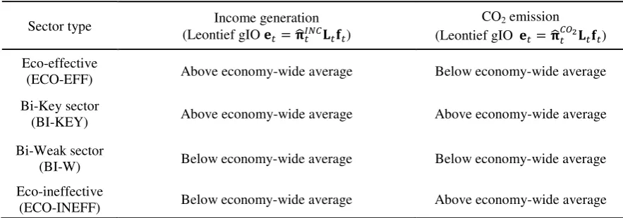
Table 1. Sectoral classification based on backward and forward linkages.

Backward linkages

Sector type Income generation

(Leontief gIO 𝐞𝐞_𝑡𝑡=𝛑𝛑�_𝑡𝑡𝐼𝐼𝐼𝐼𝐼𝐼𝐋𝐋_𝑡𝑡𝐟𝐟_𝑡𝑡)

CO2 emission (Leontief gIO 𝐞𝐞_𝑡𝑡=𝛑𝛑�_𝑡𝑡𝐼𝐼𝐶𝐶2𝐋𝐋_𝑡𝑡𝐟𝐟_𝑡𝑡)

Eco-effective

(ECO-EFF) Above economy-wide average Below economy-wide average

Bi-Key sector

(BI-KEY) Above economy-wide average Above economy-wide average

Bi-Weak sector

(BI-W) Below economy-wide average Below economy-wide average

Eco-ineffective

(ECO-INEFF) Below economy-wide average Above economy-wide average

Forward linkages

Sector type Income generation

(Ghosh gIO 𝐞𝐞_𝑡𝑡′=𝐯𝐯_𝑡𝑡𝐆𝐆_𝑡𝑡𝛑𝛑�_𝑡𝑡𝐼𝐼𝐼𝐼𝐼𝐼)

CO2 emission (Ghosh gIO 𝐞𝐞_𝑡𝑡′ =𝐯𝐯_𝑡𝑡𝐆𝐆_𝑡𝑡𝛑𝛑�_𝑡𝑡𝐼𝐼𝐶𝐶2)

Eco-effective

(ECO-EFF) Above economy-wide average Below economy-wide average

Bi-Key sector

(BI-KEY) Above economy-wide average Above economy-wide average

Bi-Weak sector

(BI-W) Below economy-wide average Below economy-wide average

Eco-ineffective

(ECO-INEFF) Below economy-wide average Above economy-wide average

Source: Own elaboration.

Note: Linkages are given relative to their relevant economy-wide average values. Symbols in parentheses in the first column represent abbreviated names of sector types.

In addition to the simple measures of eco-efficiency defined in (8) and (9) this methodology

allows one to classify sectors of an economy according to the links between income

generation and pollutant emissions. Taking into account the possible values of the linkages in

(3)-(6) we propose the eco-efficiency-focused sectoral classification presented in Table 1.

As can be seen from Table 1 the sectoral classification proposed is based on comparing the

levels of normalized linkages. To summarize, the approach presented in this paper offers a

two-dimensional eco-efficiency measure that takes into account both the eco-efficiency

indexes defined in (8) and (9) as well as the classification scheme presented in Table 1. As a

consequence, we propose that two-prong notation should be used, according to the scheme

“abbreviated name of sector’s type + (value of efficiency index)”, e.g. for

backward-linkage-oriented results the notation ECO-EFF(1.34) will denote a backward eco-efficient sector with

the value of the efficiency index equal to 1.34.

3.5. Formulating policy implications

This methodology allows one to study the differences between sectoral eco-efficiency levels

by looking at these quantities from a different point of view compared to the traditional

DEA-based approach. For an economy with 𝑛𝑛 sectors the results of this type of analysis provide two 𝑛𝑛-element sets of linkages, both in backward- and forward-linkage-oriented cases. These values are used to calculate the efficiency indexes defined in (8) and (9) as well as to obtain

the sectoral classification described in Table 1. An interesting question in the context of

analysing the eco-efficiency of the economy as a whole is what the general pattern in the

relationship between output (e.g. income generation) and input (e.g. CO2 emission) linkages is

among the sectors operating within the economy.19 For this purpose one may study the

properties of scatterplots of the values of normalized output and input linkages.

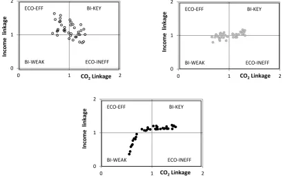
In Figure 1 we present an exemplary plot with income (i.e. the chosen output policy goal

variable) linkages on the vertical axis and CO2 (i.e. the chosen input policy goal variable)

linkages on the horizontal axis. In practical applications this plot may be interpreted in a

meaningful way. If the linkages exhibit a downward trend (upper left plot in Figure 1) it

implies that the larger the CO2-related linkage, the smaller the corresponding income-related

linkage. In other words, the sectors operating in such an economy show a tendency to emit

relatively large amounts of CO2 while having relatively low potential for income generation.

Alternatively, in the upper right plot in Figure 1 the trend is positive, suggesting that larger

CO2 emission levels are accompanied by a relatively higher potential for income generation.

19

The latter seems especially important given the rising prices of CO2 emission allowances in the EU.

However, in this particular case one still could have a significant number of eco-inefficient

sectors. From the point of view of eco-oriented policymaking the most desirable relationship

between the linkages would take the form of a nonlinear inverted-L-shaped relationship

(henceforth we will refer to such a relationship between linkages as to the ‘eco-optimal’ case).

Namely, if an economy reduced the number of ECO-INEFF sectors to zero the scatter plot of

income-CO2 linkages would look like the one presented in the bottom plot in Figure 1.20

Figure 1. Examples of two-dimensional scatterplots of input and output linkages.

Note: Linkages are given relative to their relevant economy-wide averages.

To summarize, studying the properties of two-dimensional scatterplots of datasets on input

and output linkages provides meaningful information about the eco-efficiency of the economy

examined as a whole. Taking into account the interpretation of this type of plot (comp. the

example of the linkage datasets presented in Figure 1) one may claim that from the point of

view of policymaking economies for which such output/input scatterplots exhibit a downward

trend might be interested in reversing this regularity, as a downward trend indicates the

existence of highly eco-inefficient sectors. Therefore, in a backward-linkage-oriented21 case

one may be interested in solving the following optimization problem aimed at transforming

the shape of the original scatterplot of normalized linkages towards the inverted-L-shape

20

Note that since the averages of normalized income and CO2 linkages are equal to 1, the inverted-L-shaped relationship in bottom panel of Figure 1 cannot involve only ECO-EFF and BI-KEY sectors.

21

The respective procedure in the forward-linkage-oriented case is analogous and therefore will not be repeated here.

0 1 2

0 1 2

In

co

me

l

in

ka

g

e

CO2 Linkage

0 1 2

0 1 2

In

co

me

l

in

ka

g

e

CO₂ Linkage

0 1 2

0 1 2

In

co

me

l

in

ka

g

e

CO2 Linkage

ECO-EFF BI-KEY

BI-WEAK ECO-INEFF

ECO-EFF BI-KEY

BI-WEAK ECO-INEFF

ECO-EFF BI-KEY

BI-WEAK ECO-INEFF

presented in the bottom panel of Figure 1:

OPTIMIZATION PROBLEM NO 1

Goal: Given the data on normalized output backward linkages �𝐵𝐵𝐵𝐵𝐼𝐼𝐵𝐵_{𝑖𝑖,𝑡𝑡}(𝛑𝛑𝐶𝐶𝑂𝑂𝑂𝑂,𝑡𝑡)� for output

policy target goal variable 𝛑𝛑𝐶𝐶𝑂𝑂𝑂𝑂,𝑡𝑡, and normalized input backward linkages �𝐵𝐵𝐵𝐵𝐼𝐼𝐵𝐵_{𝑖𝑖,𝑡𝑡}(𝛑𝛑𝐼𝐼𝐼𝐼,𝑡𝑡)�

for input policy goal variable 𝛑𝛑𝐼𝐼𝐼𝐼,𝑡𝑡, where 𝑖𝑖= 1, … ,𝑛𝑛 and 𝑡𝑡 stands for a fixed time point, find

shift vectors ∆_𝑡𝑡𝐶𝐶𝑂𝑂𝑂𝑂=�𝑑𝑑_𝑖𝑖𝐶𝐶𝑂𝑂𝑂𝑂,𝑡𝑡�_𝑖𝑖=1

,…,𝑛𝑛 and ∆𝑡𝑡

𝐼𝐼𝐼𝐼_=�𝑑𝑑 𝑖𝑖 𝐼𝐼𝐼𝐼,𝑡𝑡_�

𝑖𝑖=1,…,𝑛𝑛that maximize the objective

function:

𝐸𝐸𝐼𝐼𝐶𝐶_𝑆𝑆𝐼𝐼𝐶𝐶𝐹𝐹𝐸𝐸=∑ �1 + ��𝐵𝐵𝐵𝐵𝐼𝐼𝐵𝐵𝑖𝑖,𝑡𝑡�𝛑𝛑

𝐶𝐶𝑂𝑂𝑂𝑂,𝑡𝑡_�+𝑑𝑑

𝑖𝑖 𝐶𝐶𝑂𝑂𝑂𝑂,𝑡𝑡

�−1�

2��𝐵𝐵𝐵𝐵𝐼𝐼𝐵𝐵𝑖𝑖,𝑡𝑡�𝛑𝛑𝐶𝐶𝑂𝑂𝑂𝑂,𝑡𝑡�+𝑑𝑑_𝑖𝑖𝐶𝐶𝑂𝑂𝑂𝑂,𝑡𝑡�−1�−

��𝐵𝐵𝐵𝐵𝐼𝐼𝐵𝐵𝑖𝑖,𝑡𝑡�𝛑𝛑𝐼𝐼𝐼𝐼,𝑡𝑡�+𝑑𝑑𝑖𝑖𝐼𝐼𝐼𝐼,𝑡𝑡�−1�

2��𝐵𝐵𝐵𝐵𝐼𝐼𝐵𝐵𝑖𝑖,𝑡𝑡�𝛑𝛑𝐼𝐼𝐼𝐼,𝑡𝑡�+𝑑𝑑_𝑖𝑖𝐼𝐼𝐼𝐼,𝑡𝑡�−1��

𝑛𝑛

𝑖𝑖=1 ,22 (10)

assuming that −𝑙𝑙_𝑖𝑖𝑡𝑡,𝐶𝐶𝑂𝑂𝑂𝑂−≤ 𝑑𝑑_𝑖𝑖𝐶𝐶𝑂𝑂𝑂𝑂,𝑡𝑡≤ 𝑙𝑙_𝑖𝑖𝑡𝑡,𝐶𝐶𝑂𝑂𝑂𝑂+ and −𝑙𝑙_𝑖𝑖𝑡𝑡,𝐼𝐼𝐼𝐼− ≤ 𝑑𝑑_𝑖𝑖𝐼𝐼𝐼𝐼,𝑡𝑡 ≤ 𝑙𝑙_𝑖𝑖𝑡𝑡,𝐼𝐼𝐼𝐼+ for some pairs of

vectors of the upper (0≤ 𝑙𝑙_𝑖𝑖𝑡𝑡,𝐶𝐶𝑂𝑂𝑂𝑂+, 0≤ 𝑙𝑙_𝑖𝑖𝑡𝑡,𝐼𝐼𝐼𝐼+) and lower (0≤ 𝑙𝑙_𝑖𝑖𝑡𝑡,𝐶𝐶𝑂𝑂𝑂𝑂−, 0≤ 𝑙𝑙_𝑖𝑖𝑡𝑡,𝐼𝐼𝐼𝐼−) bounds and the following constraints hold true:

∑_𝑛𝑛 𝑑𝑑_𝑖𝑖𝐶𝐶𝑂𝑂𝑂𝑂,𝑡𝑡

𝑖𝑖=1 = 0, (11)

∑_𝑛𝑛 𝑑𝑑_𝑖𝑖𝐼𝐼𝐼𝐼,𝑡𝑡

𝑖𝑖=1 = 0, (12)

∑ �𝑑𝑑_𝑖𝑖𝐶𝐶𝑂𝑂𝑂𝑂,𝑡𝑡

�

𝑛𝑛

𝑖𝑖=1 ≤ 𝑀𝑀𝑡𝑡𝐶𝐶𝑂𝑂𝑂𝑂∑𝑛𝑛𝑖𝑖=1𝑚𝑚𝑎𝑎𝑥𝑥 (𝑙𝑙𝑖𝑖𝑡𝑡,𝐶𝐶𝑂𝑂𝑂𝑂−,𝑙𝑙𝑖𝑖𝑡𝑡,𝐶𝐶𝑂𝑂𝑂𝑂+), (13)

∑ �𝑑𝑑_{𝑛𝑛 𝑖𝑖}𝐼𝐼𝐼𝐼,𝑡𝑡_�

𝑖𝑖=1 ≤ 𝑀𝑀𝑡𝑡𝐼𝐼𝐼𝐼∑𝑛𝑛𝑖𝑖=1𝑚𝑚𝑎𝑎𝑥𝑥 (𝑙𝑙𝑖𝑖𝑡𝑡,𝐼𝐼𝐼𝐼−,𝑙𝑙𝑖𝑖𝑡𝑡,𝐼𝐼𝐼𝐼+), (14)

where 0≤𝑀𝑀_𝑡𝑡𝐶𝐶𝑂𝑂𝑂𝑂≤ 1, 0≤ 𝑀𝑀_𝑡𝑡𝐼𝐼𝐼𝐼 ≤1.

The objective function in (10) takes the form of a three-valued pointer indicating the sector’s

type based on the values of the modified output linkages (vertical axis) and input linkages

(horizontal axis).

Note that for eco-efficient sectors ��𝐵𝐵𝐵𝐵𝐼𝐼𝐵𝐵𝑖𝑖,𝑡𝑡�𝛑𝛑𝐶𝐶𝑂𝑂𝑂𝑂,𝑡𝑡�+𝑑𝑑𝑖𝑖𝐶𝐶𝑂𝑂𝑂𝑂,𝑡𝑡� −1�=�𝐵𝐵𝐵𝐵𝐼𝐼𝐵𝐵𝑖𝑖,𝑡𝑡�𝛑𝛑𝐶𝐶𝑂𝑂𝑂𝑂,𝑡𝑡�+𝑑𝑑𝑖𝑖𝐶𝐶𝑂𝑂𝑂𝑂,𝑡𝑡� −1

and ��𝐵𝐵𝐵𝐵𝐼𝐼𝐵𝐵𝑖𝑖,𝑡𝑡�𝛑𝛑𝐼𝐼𝐼𝐼,𝑡𝑡�+𝑑𝑑𝑖𝑖𝐼𝐼𝐼𝐼,𝑡𝑡� −1�=−��𝐵𝐵𝐵𝐵𝐼𝐼𝐵𝐵𝑖𝑖,𝑡𝑡�𝛑𝛑𝐼𝐼𝐼𝐼,𝑡𝑡�+𝑑𝑑𝑖𝑖𝐼𝐼𝐼𝐼,𝑡𝑡� −1�. Thus, for these sectors one

has 𝐸𝐸𝐼𝐼𝐶𝐶_𝑆𝑆𝐼𝐼𝐶𝐶𝐹𝐹𝐸𝐸 = 2. Similarly, for sectors of type BI-KEY and BI-WEAK one has 𝐸𝐸𝐼𝐼𝐶𝐶_𝑆𝑆𝐼𝐼𝐶𝐶𝐹𝐹𝐸𝐸 = 1, while for sectors of type ECO-INEFF one has 𝐸𝐸𝐼𝐼𝐶𝐶_𝑆𝑆𝐼𝐼𝐶𝐶𝐹𝐹𝐸𝐸 = 0.23

22_|𝑥𝑥|

stands for absolute value of 𝑥𝑥. 23

The fact that for 𝐸𝐸𝐼𝐼𝐶𝐶_𝑆𝑆𝐼𝐼𝐶𝐶𝐹𝐹𝐸𝐸= 1 both for BI-KEY and BI-WEAK sectors seems to stand in line with the idea of linkage-based measures of eco-efficiency defined in (8) and (9). Namely, the relative impact of BI-WEAK sectors on the economy-wide generation of income and CO2 is similar to the analogous relative impact of BI-KEY sectors. If the income generating potential and the CO2 emission potential of a sector are both below the respective economy-wide-averages, the net income of such a sector (i.e. the income less environmental costs) per unit of product is similar to the corresponding ratios calculated for BI-KEY sectors.

Conditions (11) and (12) ensure that the modified linkages remain normalized. To make the

overall change in linkages more realistic we follow the arguments of Gurgul and Lach

(2018c) and assume (comp. (13), (14)) that the overall change of input and output linkages

cannot exceed a chosen threshold level (i. e.𝑀𝑀_𝑡𝑡𝐶𝐶𝑂𝑂𝑂𝑂 for output linkages and 𝑀𝑀_𝑡𝑡𝐼𝐼𝐼𝐼 for input

linkages) of the maximal possible change (i. e.∑𝑛𝑛_𝑖𝑖=1𝑚𝑚𝑎𝑎𝑥𝑥 (𝑙𝑙_𝑖𝑖𝑡𝑡,𝐶𝐶𝑂𝑂𝑂𝑂−,𝑙𝑙𝑡𝑡_𝑖𝑖,𝐶𝐶𝑂𝑂𝑂𝑂+)for output linkages

and ∑𝑛𝑛_𝑖𝑖=1𝑚𝑚𝑎𝑎𝑥𝑥 (𝑙𝑙_𝑖𝑖𝑡𝑡,𝐼𝐼𝐼𝐼−,𝑙𝑙_𝑖𝑖𝑡𝑡,𝐼𝐼𝐼𝐼+) for input linkages). This assumption implies that not all changes

in normalized linkages may reach maximal absolute values at the same time. As suggested by

Gurgul and Lach (2018c), in such a case the optimal solution to OPTIMIZATION PROBLEM NO

1 will point out only the most important linkages in terms of transforming the actual relationship between linkages towards the eco-optimal inverted-L-shape presented in the

bottom plot in Figure 1.

3.6. Practical implementation

Another important problem is the practical implementation of the solution to OPTIMIZATION

PROBLEM NO 1. The latter takes the form of two lists of modified linkages, i.e.

��𝐵𝐵𝐵𝐵𝐼𝐼𝐵𝐵𝑖𝑖,𝑡𝑡�𝛑𝛑𝐶𝐶𝑂𝑂𝑂𝑂 ,𝑡𝑡

�+𝑑𝑑_𝑖𝑖𝐶𝐶𝑂𝑂𝑂𝑂,𝑡𝑡��

𝑖𝑖=1,…,𝑛𝑛 and ��𝐵𝐵𝐵𝐵𝐼𝐼𝐵𝐵𝑖𝑖,𝑡𝑡�𝛑𝛑

𝐼𝐼𝐼𝐼,𝑡𝑡

�+𝑑𝑑_𝑖𝑖𝐼𝐼𝐼𝐼,𝑡𝑡��

𝑖𝑖=1,…,𝑛𝑛. Therefore, in order

to translate the solution to OPTIMIZATION PROBLEM NO 1 into a set of practical policy recommendations one must know what policies should be taken in order to influence the

output and input linkages of particular sectors within an economy. In general, for each type of

linkage measures two general answers may be given to this question. To illustrate the two

respective policies let us focus on the case of increasing the traditional output backward

linkage for a particular sector 𝑖𝑖₀.24

Policies for changing the traditional backward linkages of sector 𝑖𝑖₀

 Strategy 1: Modifying the policy goal variable 𝛑𝛑𝐶𝐶𝑂𝑂𝑂𝑂,𝑡𝑡

As shown in (3):

�𝐵𝐵𝐵𝐵𝐼𝐼𝐵𝐵𝑖𝑖0,𝑡𝑡�𝛑𝛑𝐶𝐶𝑂𝑂𝑂𝑂 ,𝑡𝑡

��=�∑𝑛𝑛_𝑘𝑘=1𝜋𝜋_𝑘𝑘𝐶𝐶𝑂𝑂𝑂𝑂,𝑡𝑡𝑙𝑙_{𝑘𝑘𝑖𝑖}𝑡𝑡 ₀�, (15)

and

�𝐵𝐵𝐵𝐵𝐼𝐼𝐵𝐵𝑖𝑖0,𝑡𝑡�𝛑𝛑𝐼𝐼𝐼𝐼 ,𝑡𝑡

��=�∑𝑛𝑛_𝑘𝑘=1𝜋𝜋_𝑘𝑘𝐼𝐼𝐼𝐼,𝑡𝑡𝑙𝑙𝑡𝑡_{𝑘𝑘𝑖𝑖0}�. (16)

In other words, the traditional backward linkages for sector 𝑖𝑖₀ take the form of a scalar

24

The respective procedure in a forward-linkage-oriented case is analogous to the backward-oriented scheme, therefore will not be repeated here.