Munich Personal RePEc Archive
Testing the Friedman and Schwartz
Hypothesis using Time Varying
Correlation Analysis
Ghosh, Taniya and Parab, Prashant Mehul
IGIDR
22 November 2018
Testing the Friedman and Schwartz Hypothesis using Time Varying
Correlation Analysis
November 22, 2018
Taniya Ghosh (Corresponding Author)
Indira Gandhi Institute of Development Research (IGIDR), Gen. A. K. Vaidya Marg, Filmcity
Road Mumbai, 400065, India, Email Add.: taniya@igidr.ac.in, Tel.:91-22-28426536
ORCID ID: https://orcid.org/0000-0002-9792-0967
Prashant Mehul Parab
Indira Gandhi Institute of Development Research (IGIDR), Gen. A. K. Vaidya Marg, Filmcity
Testing the Friedman and Schwartz Hypothesis using Time Varying
Correlation Analysis
Abstract
The study analyses the time varying correlation of money and output using DCC GARCH model
for Euro, India, Poland, the UK and the USA. In addition to simple sum money, the model uses
Divisia monetary aggregate, theoretically shown as the actual measure of money. The inclusion
of Divisia money restores the Friedman and Schwartz hypothesis that money is procyclical. Such
procyclical nature of association was not robustly observed in the recent data when simple sum
money was used.
Keywords: DCC GARCH,Divisia, Monetary Aggregates, Real Output
1. Introduction
A natural way to analyse the link between money and output is to examine the statistical
correlation between them. The influential paper of Friedman and Schwartz (1963a) established
the statistical link between money and business cycles more than 50 years ago. They found
money to be procyclical using the historical US data. However, this close association was
volatility (Friedman and Kuttner, 1992; Estrella and Mishkin, 1997). Moreover, the rampant
financial innovations made the measure of money using simple sum unreliable.
After the great financial crisis (GFC), however, there was a resurgence of studies focusing on
role of money, especially Divisia money. This is due to interest rate losing its credibility as the
reliable monetary policy instrument when it could not be lowered further. The literature on
aggregation-theoretic Divisia monetary aggregates argue that Divisia money puts weights on
different components of money based on their relative liquidity capturing the liquidity in the
economy accurately when new instruments are introduced (Belongia and Binner, 2001; Barnett,
1980).
Belongia and Ireland (2016), using the recent US data, have found procyclical correlations
between money and output as Friedman and Schwartz (1963a). The results are significant when
Divisia money is used instead of simple sum. Hendrickson (2014) invalidated the redundant role
of money as an intermediate target or as an informational variable by estimating a stable money
demand equation using Divisia. He demonstrated that Divisia money Granger-cause output while
simple sum does not.
Engle’s (2002) dynamic conditional correlation (DCC) GARCH model is used to capture the
time varying role of money. We find that1 (1) Divisia money growth rates are mostly procyclical,
(2) money is countercyclical during recessions, (3) the unconventional monetary policy measures
of the US and the UK can explain money’s transient countercyclicality during GFC (4) Euro’s
1
delay in implementing such measures and the sovereign debt crisis reflected in Divisia money’s
persistent countercyclicality post GFC, and (5) the inclusion of Divisia money establishes that
money still is a reliable business cycle indicator.
2. Data and Methodology
The monthly data for simple sum M3 and industrial production (used as a proxy for real output)
is taken from OECD database. The Divisia data are obtained from respective central bank’s
website except India and Euro whose Divisia data are taken from Ramachandran et. al. (2010)
and Darvas (2015), respectively.
Let where is a 2 x 1 vector where denotes industrial production and
denotes money supply (simple sum or Divisia). Levels of all the variables are non-stationary
while the annualized month-on-month log differences (growth rate) are stationary (appendix
table 1A). Since GARCH models analyse volatility of a data with zero (constant) mean, such
transformation to growth rates gives stationary heteroscedastic data for analysis.
The conditional mean equation of the model is:
A(L)Xt=εt, εt|It-1 ~ N(0,Ht) (1)
where εt is the vector of error terms and It-1 is the information set available till time t-1. is the
conditional variance-covariance matrix of the error represented as:
(2)
where is a time-varying diagonal matrix obtained from univariate GARCH(p,q) models such
∑ ∑ (3)
The DCC (M,N) GARCH(p,q) model comprises of the following equations:
(4)
Where
( ∑ ∑ ) ̅ ∑ ∑ (5)
Where ̅ is the variance-covariance matrix which is time invariant and Qt*-1 is the diagonal
matrix of square root of elements of Qt. Hence, can be represented as: √
3. Results
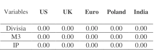
The null hypothesis for Lagrange multiplier tests assumes the series to be homoscedastic. All the
variables display heteroscedasticity, deeming them fit for a GARCH analysis.2
DCC(1,1)-GARCH(1,1) model is estimated using the quasi maximum likelihood estimation (QMLE)
technique. The key parameters, dcca1 and dccb1, denoted by the coefficients and in
equation (5), are presented in table 3A in appendix for .3 We find significant in
all cases validating the use of DCC model. Also, + > 0 for all the countries with being
closer to 1 implies a high persistence in the correlation. + closer to 1 shows that the
conditional variances are highly persistent and mean reverting in nature. We run post estimation
diagnostics using weighted Portmanteau test (Li and Mak (1994)) on individual error terms as
well as the cross products of the residuals (Tse and Tsui, 2002)4. We find the absence of
2 See Table 2A (appendix), null is rejected at 1% level of significance.
3 Table 3A presents the conditional mean and the conditional variance equations.
heteroscedasticity in all the cases except for the cross products of the residuals for simple sum
money for Euro.
Left (right) panel of figure 1 captures the correlation of output with Divisia money growth
(simple sum M3 growth) with 95% confidence intervals. Divisia money shows procyclicality in
general and countercyclicality during recessions. The simple sum money growth, however, fails
to capture the procyclical relation robustly. Correlations with simple sum have largely remained
negative post GFC for the UK, and there were frequent countercyclical episodes for both the US
starting 1990s and for India for the entire sample.
The graphs show a systematic and predictable behavior of money and output correlation
especially before, during and after any major recession. There is a sharp decline in the
correlation during GFC and in many cases it becomes countercyclical. Post GFC, the correlation
with Divisia money becomes positive and even reaches the pre-recession level for all the
countries5. Euro showed persistent countercyclicality of Divisia during GFC and in its aftermath
while UK and US showed transient countercyclicality. Interestingly, US and UK started pursuing
quantitative easing immediately after the onset of GFC, while Euro delayed it for several years.
US Divisia, consistent with Belongia and Ireland (2016) remained procyclical, with exceptions
of the GFC, the energy crisis of late 1970s and the early 1980s recessions. UK Divisia became
countercyclical around 2002 when Euro was formed and around 2016 when England voted to
exit out of Euro (Brexit). Although, Euro’s correlation between Divisia money and output fell
during the Brexit movement, it did not become countercyclical. Brexit did not have an adverse
impact on correlations of Euro, although the GFC and the period ensuing that, did. For Poland
and India, the Divisia money was mostly highly procyclical.
[INSERT FIGURE 1 HERE]
4. Conclusion
We evaluate the shifts in money and output correlation for Euro, India, Poland, the UK and the
US by estimating a bivariate DCC-GARCH model. Divisia money growth largely remains
procyclical. Most of the simple sum money results are obscured by money’s frequent
countercyclical behavior. Money’s countercyclicality during recessions hints at shifting
preference behavior of individuals for demand for liquid assets. The quantitative easing adopted
by the US and the UK during GFC was deemed effective as it helped money become procyclical
much faster compared to Euro which did not adopt the measure sooner.
References:
Barnett, W.A., 1980, “Economic Monetary Aggregate: An Application of Index Number and
Aggregation Theory”. Journal of Econometrics, September, 1980.
Belongia, M. and Binner, J., 2001, Divisia Monetary Aggregates: Theory and Practice, Palgrave
Macmillan, UK.
Belongia, M.T. and Ireland, P.N., 2016, “Money and Output: Friedman and Schwartz Revisited”,
Journal of Money, Credit and Banking, Vol. 48, No. 6.
Darvas, Z., 2015, “Does Money Matter in the euro Area? Evidence from a New Divisia Index”,
Engle, R., 2002, “Dynamic Conditional Correlation: A Simple Class of Multivariate Generalized
Autoregressive Conditional Heteroskedasticity Models”, Journal of Business & Economic
Statistics, Vol. 20, No. 3, DOI 10.1198/073500102288618487.
Estrella, A. and Mishkin, F. S., 1997, “Is there a role for monetary aggregates in the conduct of
monetary policy?” Journal of Monetary Economics, Vol. 40, p. 279 304.
Friedman, B. M. and Kuttner, K. N., 1992, ”Money, Income, Prices, and Interest Rates.”
American Economic Review, Vol. 82, No. 3, p. 472 - 492.
Friedman, M., and Schwartz., A. J., 1963a, “Money and Business Cycles.’’ Review of Economics
and Statistics, 45, 32–64.
Hendrickson, J. R., 2014, “Redundancy and ‘Mismeasurement’? A Reappraisal of Money”,
Macroeconomic Dynamics, Volume 18, pp. 1437–65.
Li, W. K. and Mak, T. K., 1994. On the squared residual autocorrelations in nonlinear time series
with conditional heteroskedasticity, Journal of Time Series Analysis, 15(6), 627 – 636.
Ramachandran, M., Das, R., and Bhoi, B., 2010, “The Divisia Monetary Indices as Leading
Indicators of Inflation”, RBI Development Research Group Study No. 36, Mumbai.
Tse, Y. K., and Tsui, A. K. C., 2002, “A Multivariate GARCH Model with Time-Varying
Appendix:
Table 1A- Augmented Dickey Fuller Tests
Null: Variable has a unit root
US (1967 Feb - 2018 June)
UK (1999 Feb - 2018 June)
Euro Area ( 2001 Feb - 2018 June)
Variables
Level First Difference Level First Difference Level First Difference
Divisia -0.51 -12.69* 1.83 -11.79* -0.34 -6.70*
M3 5.36 -10.09* -1.48 -8.84* -0.94 -5.18*
IP -1.57 -11.89* -1.55 -12.19* -1.52 -8.51*
Poland (1997 Jan- 2018 June)
India (1994 Apr - 2008 June)
Divisia 2.22 -10.27* 2.63 -9.51*
M3 -0.22 -14.26* 4.82 -10.93*
IP -2.19 -13.85* 1.78 -11.09*
Table 2A- Lagrange Multiplier Test
Null: Series is homoscedastic (p-values are reported)
Variables US UK Euro Poland India
Divisia 0.00 0.00 0.00 0.00 0.00
M3 0.00 0.00 0.00 0.00 0.00
IP 0.00 0.00 0.00 0.00 0.00
Table 3A- Conditional Mean and Conditional Variance Equations
US UK EURO
Divisia(t) IP (t) M3(t) IP (t) Divisia(t) IP (t) M3(t) IP (t) Divisia(t) IP (t) M3(t) IP (t)
Co nd it io na l M ea
n Constant 5.79* 2.99* 6.03* 3.02* 9.17 -0.12 5.79* -0.12 5.16* 1.63* 6.78* 1.63*
Divisia(t-1) 0.41* -0.57* 0.78* 0.78* 0.73* 0.15* 0.09 0.19 0.96* -0.24** 0.98* -0.24** IP(t-1) -0.69* 0.72* -0.22** -0.60* -0.18* -0.22 0.92* -0.46*** 0.80* -0.09 -0.82* -0.09
Co nd it io na l Va ria nce
Constant 0.84* 23.44* 5.85* 23.83* 0.76 49.91 2.26 58.27 0.42 102.71* 1.41* 102.71*
α (1) 0.19* 0.31* 0.63* 0.31* 0.06*** 0.48* 0.001 0.38* 0.03 0.32** 0.07 0.32**
β(1) 0.84* 0.34** 0.16 0.33** 0.93* 0.16 0.94* 0.15 0.94* 0.00 0.86* 0.00
dcca1 0.006 0.006 0.008 0.03 0.05 0.03
dccb1 0.84* 0.85* 0.82* 0.81* 0.84* 0.83*
POLAND INDIA
Co nd it io na l M ea n
Constant 9.52* 4.92* 11.67* 5.02* 14.59* 7.70* 15.94* 7.45*
Divisia(t-1) -0.48* 0.20 0.06 -0.28** 0.30* 0.23** 0.45* -0.50* IP(t-1) 0.26* 0.76* -0.34** -0.12 -0.26** -0.08 -0.35* -0.02*
Co nd it io na l Va ria nce
Constant 0.00 0.00 0.00 0.00 6.48 4.36* 2.37* 6.25*
α (1) 0.02 0.03 0.02 0.03 0.05 0.1*** 0.08 0.07***
β(1) 0.97* 0.97* 0.97* 0.96* 0.91* 0.89** 0.85* 0.91*
dcca1 0.09** 0.12* 0.04 0.03
dccb1 0.66* 0.53* 0.83* 0.85*
Table 4A- Li-Mak Test for Heteroscedasticity
Null Hypothesis: Series is homoscedastic
US UK EURO POLAND INDIA
Divi sia
Simple Sum
Divi sia
Simple Sum
Divi sia
Simple Sum
Divi sia
Simple Sum
Divi sia
Simple Sum Money residual 0.99 0.99 0.99 0.27 0.22 0.51 0.99 0.43 0.99 0.91
IP residual 0.99 0.99 0.99 0.49 0.15 0.94 0.82 0.99 0.88 0.99
Cross-product
Figure 1: Money Growth and Output Growth Correlations US
EURO
POLAND