Forecasting GDP: Do Revisions Matter?

Munich Personal RePEc Archive

Forecasting GDP: Do Revisions Matter?

Check, Adam J. and Nolan, Anna K. and Schipper, Tyler C.

University of St. Thomas, University of St. Thomas, University of

St. Thomas

1 April 2018

Online at

https://mpra.ub.uni-muenchen.de/86194/

Forecasting GDP: Do Revisions Matter?

Adam J. Check

University of St. Thomas

Anna K. Nolan

University of St. Thomas

Tyler C. Schipper

April 2018

Abstract

This paper investigates the informational content of regular revisions to real GDP growth and its components. We perform a real-time forecasting exercise for the advance estimate of real GDP growth using dynamic regression models that include GDP and GDP component revisions. Echoing other work in the literature, we find little evidence that including aggregate GDP growth revi-sions improves forecast accuracy relative to an AR(1) baseline model; however, when we include revisions to components of GDP (i.e. C, I, G, X, and M) we find improvements in forecast accuracy. Overall, nearly 68% of all models that contain subsets of component revisions outperform our baseline model. The “best” component-augmented model forecasts roughly 0.2 percentage points better, and a large subset of models improve RMSFE by more than 5%. Fi-nally, we use Bayesian model comparison to demonstrate that differences in forecast performance are unlikely to be the result of statistical noise. Our results imply that component revisions, in particular to consumption, contain important information for forecasting GDP growth.

Keywords: Data revisions, real-time data, forecasting

JEL Classification Numbers: E01, C11, C53, C82

∗_{Correspondence for this paper can be sent to Tyler Schipper at} [email protected]_{. We}

1

Introduction

The revision process for many macroeconomic time series has led to an explosion

of work focusing on the use of real-time data. Two aspects of real-time data are

particularly important for forecasting. First, many studies investigate how the use

of real-time data impacts the evaluation of forecast performance (e.g. Robertson and

Tallman, 1998; Croushore and Stark, 2003; Faust et al., 2003). Estimating a

fore-casting model using post-revision data available to the researchertoday may create a

misleading comparison with forecasts from a model based on the best available data

at the time they were made. Second, real-time data has given rise to approaches that

use multiple vintages of the same time series to improve forecast performance (e.g

Howrey, 1978; Clements and Galv˜ao, 2012).

In light of this important work with real-time data, we ask whether revisions to

GDP growth contain information that can help forecast advance estimates of GDP

growth. We investigate the informational content of both aggregate revisions to

GDP and revisions to its components. Echoing other work in the literature, we find

that revisions to GDP growth have no impact on short-run forecast accuracy.

How-ever, there is strong evidence that revisions to certain GDP components, principally

consumption, have important information for forecasting economic growth. Further,

the improvement in forecast accuracy can be substantial over an AR(1) benchmark

model. Nearly 68% of all models that contain subsets of component revisions

outper-form the baseline model. The “best” component-augmented model forecasts roughly

0.2 percentage points closer to the advance estimate of GDP growth than an AR(1).

There is a well-developed literature that has attempted to incorporate preliminary

data into coherent forecasting frameworks.1 _{Much of its focus has been on forecasting} 1

post-revision releases and measuring the efficiency of early data releases. In this vein,

Howrey (1978) outlines a method to efficiently use preliminary data when errors in

measuring GDP are serially correlated. Kishor and Koenig (2012) generalize Howrey

(1978) by also allowing data revisions to be efficient estimates with white-noise errors

as in Sargent (1989). State-space forecasting models have also had mixed results

in forecasting post-revision data using data revisions (Croushore, 2006). Finally,

Clements and Galv˜ao (2012) investigate the use of vintage-based VARs (V-VARs)

to forecast post-revision data.

Our work more closely aligns with a strain of the literature that has looked at

forecasting early or advance estimates of macroeconomic time series. We

incorpo-rate the findings of Koenig et al. (2003) who emphasize that forecasting advance

releases of GDP growth is best done using only advance releases in the estimation of

forecasting models. Two other studies align closely with our objectives in that they

attempt to incorporate information from revisions and forecast advance GDP growth:

Clements and Galv˜ao (2013a) and Clements and Galv˜ao (2013b). The former paper

concludes that several variants of vintage-based VAR (V-VAR) models show little

improvement in forecast accuracy. Clements and Galv˜ao (2013b) suggest a real-time

vintage approach to forecasting. Using this approach, they estimate models using

lightly revised data while their forecasts are conditioned on the same data as

tradi-tional approaches to forecasting that utilize the most recent vintage. Their approach

yields small improvements in forecast accuracy. Our method contrasts nicely with

Clements and Galv˜ao (2013b) in that we also forecast the advance estimate of GDP

growth, but our forecasts are conditioned on the same series used for estimation.

Our first set of results are established in a straight-forward forecasting exercise.

We use dynamic regression models to produce one-period ahead forecasts of advanced

(aggre-gate or components) and estimate the model using maximum likelihood. We evaluate

forecast performance using root mean squared forecasting error (RMSFE) and check

for robustness across other accuracy measures, data assumptions, and test periods.

Our forecasting framework is simpler than previous approaches in that we do not

attempt to estimate using multiple vintages of GDP, but rather incorporate revisions

themselves as additional right-hand side variables in our dynamic regression models.

We refrain from an a priori elimination of component-based models leaving us

with a large set of potential models to consider. Given our priors and the existing

literature, there was little justification for concluding that some components were

more important than others. Our second set of results addresses this large model

space problem. To test the significance of our findings in the presence of many

alternative models, we turn to Bayesian model comparison. Even with strong priors

that our baseline model should outperform component-based models, we find that

the posterior probability of our baseline model falls. There is a high probability that

the superior forecasting model (in the large set that we consider) contains at least

one component revision. Our Bayesian analysis demonstrates that the difference in

forecast performance is unlikely to be the result of statistical noise.

Beyond highlighting the fact that component revisions contain information that

improves forecast performance, these results may have important implications for

other questions on real-time data including the efficiency of early estimates and

whether revisions contain news or reflect statistical noise. The remainder of this

paper is organized as follows. Section 2 outlines our data and how we evaluate

forecast performance in both frequentist and Bayesian frameworks. Section 3 presents

our primary findings and tests their robustness. It also addresses the significance of

our findings in the context of our large set of alternative models. Finally, Section 4

2

Data and Estimation

We use advance estimates of real GDP growth over the period 1991Q4:2017Q1.

Be-ginning in 1991Q4, the BEA began to follow the current release schedule composed

of three regular releases of GDP: advance, second, and third. The advance

esti-mate of real GDP growth is calculated as the percentage change between the new

advanced estimate of GDP and the third estimate of the previous quarter’s GDP.

We use this standard construction as it is the headline measure reported by the

Bu-reau of Economic Analysis (BEA), and therefore the most likely to impact markets

and monetary policy. All of our real-time data is from the Real-Time Data Set for

Macroeconomics which is housed at the Federal Reserve Bank of Philadelphia. A

brief description of the construction for our variables is available in Appendix A.

Relevant summary statistics for our data can be found in Appendix B.

We supplement our GDP growth data with data on aggregate GDP revisions

(henceforth simply aggregate revisions) and revisions to consumption, government

spending, investment, imports, and exports (denoted asc, g, i, m, andxrespectively).

The advance components for quartert are measured as the percentage change in the

expenditure category between the third release for quarter t −1 and the advance

release for quarter t. Therefore, they are measured in an equivalent way to our

advance GDP growth measure. However, we do not use these components directly,

since the goal of our study is to determine if revisions contain useful information for

future values of GDP growth. Therefore, in our estimation procedure, we instead

include up to two revisions for GDP growth or each component’s growth. First

revisions are the difference between the advanced estimate of growth and the second

estimate, and second revisions are the difference between the second estimate of

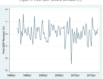
Figure 1: First GDP Growth Revision (r1)

The first revision to GDP is measured as the difference in the annualized growth rates of the advance and second releases of GDP.

for each revision. For example, the first consumption revision, c1, is the percentage

point difference between consumption growth in the advance release and consumption

growth in the second release. As an example, Figure 1 plots the first revision to

GDP growth. In total, we have two aggregate revisions and ten different component

revisions that can be used to augment our dynamic regression models of GDP growth.

Our main goal is to investigate whether the inclusion of revisions in a linear

regression model increases forecast performance relative to a baseline AR(1) model.2 2

The use of ARMA(p,q) models as a baseline is quite common (e.g Koop and Potter,

2004; Koenig et al., 2003), although the mechanism for choosing the lag lengths

depends on the application. We do not argue that our baseline is thebest model for

forecasting GDP growth, but rather that forecast improvements beyond this baseline

are evidence of revisions containing information about future GDP growth. To do so,

we consider models spanning all possible combinations of component revisions. With

k= 10 total types of component revisions, we have R= 210 _{= 1,024 possible models}

to consider.3

Let any specific model be denoted by Mr ∈ {M1, M2,· · ·, M1024}.

Under a specific model, Mr, we consider one unique subset of revisions, Xr, with

coefficient estimates,µr andβr, and AR(1) persistence estimate,ρr. Our state-space

model with AR(1) errors under model r at time t is then given by:

yt=µr+Xtr−1βr+η

r

t (1)

η_tr=ρrηrt−1+ε

r

t (2)

whereεr_t ∼N(0, σr). In our baseline model we do not include any revisions, so Xtr−1

is empty and equations (1) and (2) represent a standard AR(1) process.

All models are initially estimated on the sample period 1991Q4:2004Q3. This

period roughly splits our data, so that we use the second half of the data as our

test sample. Beginning our test sample in 2004Q4 allows us to measure forecast

performance during the Great Recession (2008Q1:2009Q2). It also leaves a relatively

large amount of time between the start of our sample in 1991Q4 and the beginning

of our test data in 2004Q4. This gap in time helps to diminish the impact of the

coefficient priors in our Bayesian model comparison exercise. While we think that

3

beginning the forecasting exercise in 2004Q4 is sensible, we also show that our results

are robust to the choice of test sample.

When forecasting, we use both frequentist and Bayesian techniques. First, we

investigate forecast performance of various revision-augmented models as measured

by RMSFE under maximum likelihood estimation, since this is a standard way to

assess forecasting performance. We then switch to using Bayesian techniques for

two primary reasons: (1) most frequentist statistical tests of forecast performance

require that the forecast models be non-nested, and (2) Bayesian techniques

pro-vide a relatively simple and theoretically justified way to compute posterior model

probabilities using the forecast performance of the models. Since maximum

likeli-hood estimation of conditionally linear ARMA models is widely understood, we omit

further discussion. Instead, we focus on our Bayesian estimation procedure.

2.1

Bayesian Estimation

As is well documented in the Bayesian literature, for each modelMr, we can compute

the model probability,p(Mr|Y) as:

p(Mr|Y) = cp(Y|Mr)p(Mr) (3)

wherep(Mr|Y) is the probability of modelrconditional on the data,Y. This is

com-monly called the posterior probability of model r. Defined in this way, the posterior

probability represents the probability that, of the set of models under consideration,

model Mr is the best model for explaining the data. There are three terms on the

right-hand side that together determine this probability: c is a constant, p(Y|Mr)

is the marginal likelihood of modelr, andp(Mr) is the prior probability assigned to

for the inclusion of irrelevant variables.4

2.1.1 Model Priors

Before computing model probabilities, we need to specify the model priors, p(Mr)

for each model. Since parsimonious models, like an AR(1), have shown relatively

strong forecast performance in many studies of various macroeconomic indicators,

we set 50% of our prior belief on the AR(1) model. The other 50% prior probability

is spread across all remaining models in a geometrically declining fashion according

to model size. That is, we believe with roughly 25% prior probability that a model

that includes any single component revision by itself will be the superior forecasting

model, with roughly 12.5% probability that a model with any combination of two

component revisions will be the superior forecasting model, etc. This is consistent

with our belief that parsimonious forecasting models are preferred to more complex

ones.

Mathematically, the prior probability of model Mr depends on the number of

component revisions, kr, that are included in that model. For all models with at

least one revision included, we set:

p(Mr|kr =j)∝

0.5j+1

Nj

Nj =

10

j

j ∈ {1,· · · ,10}.

For example, the group of models with only one component revision have a collective

4

It may be helpful to think ofp(Y|Mr) as akin to AIC or BIC, as it includes a built in penalty

for large models. In fact, the large sample approximation top(Y|Mr) under linear regression is

−1

prior probability of roughly 25%. We divide this prior probability equally across all

models that include only one revision. Since there are 10 of these models, each

one-component revision model receives a prior probability of roughly 2.5%. In addition

to the model priors, each particular model has priors on the regression coefficients

and the AR(1) term in the error equation. Since we are considering 1,024 models,

this is hard to do in a model-by-model way. Instead, we assign these prior beliefs

in an automatic and fairly standard fashion. Additional details can be found in

Appendix C.

2.1.2 Forecast Performance

Since this study is primarily concerned with forecast accuracy and the informational

content of revisions, we alter Equation (3) so that the posterior model probabilities

are based on forecast performance rather than in-sample fit. To do this, we replace

the marginal likelihood, p(Y|Mr), in Equation (3) with a measure of forecast

per-formance: the one-step-ahead predictive density, a measure of the performance of

the entire forecast distribution. As shown in Amisano and Geweke (2017), the sum

of the log of one-step-ahead predictive densities starting from the first in-sample

observation is actually equal to the log marginal likelihood:

ln[p(Y|Mr)] = T X

t=0

ln[p(yt+1|Mr, yt)]

where the forecast made att = 0 for the data in periodt = 1 comes solely from the

priors of the model. Therefore, if used over the entire sample, the two measures will

produce identical model probabilities. However, to maintain consistency with the

previous section, we focus on our test period of 2004Q4:2017Q1. Instead of using

from each model, denoted as pdr, starting after τ = 2004Q3:

pdr = T X

t=τ

ln[p(yt+1|Mr, yt)]

PDr = exp{pdr}

This measure: (1) summarizes forecasting performance, (2) diminishes the impact of

the priors that we place on the regression coefficients, and (3) can be used to form

model probabilities. An additional benefit of using the log predictive density instead

of the marginal likelihood is that it prevents the probability on any single model

from approaching 100% too quickly, which can be sub-optimal if the “true” model is

not under consideration.5

To form the model probabilities with this measure, we compute:

p(Mr|Y) = cPDr p(Mr) (4)

We use these model probabilities to determine the strength of evidence for the

base-line AR(1) model relative to dynamic regression models that are augmented with

GDP or component revisions. If the component revisions are not important for

fore-casting GDP growth, we would expect the posterior probability of the AR(1) model

to either increase from its prior probability or to at least remain large relative to the

posterior probabilities of models that include component revisions.

The estimation process is as follows. First, we focus on one model, Mr from

the set {M1, M2,· · · , M1024}. This model will have a unique set of regressors, Xr.

Given that our test sample starts in 2004Q4, we use the subset of our data from

the first observation through 2004Q3 to estimate the posterior distribution

regres-5

sion coefficients, P r(βr,t|, yt, Mr). Using this distribution of coefficient estimates,

along with the posterior distribution for the AR(1) coefficient and the variance of

the error term, we form the one-period-ahead out-of-sample forecast distribution,

p(yt+1|Mr, yt). We then forward the end-date of the training sample by one period,

so that it runs through 2004Q4, and repeat the estimation and forecasting process.

We continue in this fashion until we reach the end of our sample. We then move

to the next model, Mr+1 and repeat the process. This process yields point-forecasts

and forecast distributions under each possible model that are used to evaluate

Equa-tion (4).

3

Results

We present our results in four sections. The first two document the main results of

this paper: aggregate revisions do not improve forecast performance, while

compo-nent revisions have important information regarding future real GDP growth. The

third section investigates the robustness of our main results, and the final section

addresses the statistical significance of these results given the large number of models

considered.

3.1

Aggregate Revisions

Our first set of results investigates whether aggregate revisions to real GDP growth

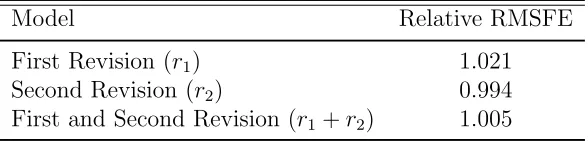
can improve forecast performance over our baseline model. Table 1 presents the

relative forecast performance for three models that are augmented with aggregate

revisions. None of the three models show meaningful improvements in forecast

vintage-based VARs do not improve forecast accuracy for advance estimates of real

GDP growth. It is important to note that these aggregate revisions are themselves

composed of component revisions that may be the result of very different data

gener-ating processes. This aggregation process may obfuscate the important information

contained in any individual component revisions. Hence, it is worth investigating

the contribution of individual components to forecasting real GDP growth.

Table 1: Forecasting with Aggregate Revisions

Model Relative RMSFE

First Revision (r1) 1.021

Second Revision (r2) 0.994

First and Second Revision (r1+r2) 1.005

The first column indicates the covariates that are included in Equation (1). RMSFE is reported relative to the baseline AR(1) model.

3.2

Component Revisions

In comparison to aggregate revisions, revisions to individual components increase

forecast performance and therefore appear to contain information that is

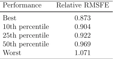
impor-tant for forecasting the advance release of real GDP growth. Table 2 highlights the

relative forecast performance for several models. The best model in terms of

fore-cast performance has RMSFE that is nearly 13% below that of the baseline model.

This improvement is not limited to a small subset of models. More than half of all

component-based models outperformed the baseline model by at least 3.1%. These

results are surprising and important on two fronts. First, they indicate the revisions

what is captured by past GDP growth. Second, this information is typically hidden

through the aggregation process.

Table 2: Forecasting with Component Revisions

Performance Relative RMSFE

Best 0.873

10th percentile 0.904 25th percentile 0.922 50th percentile 0.969

Worst 1.071

Performance refers to how a model did relative to the entire distribution of 1024 component-based models. For instance, the 10th percentile model is the 102nd best performing model in terms RMSFE. Relative RMSFE in column two reports each model’s forecast performance rela-tive to the baseline AR(1) model. The “best” forecasting model contains revision to components

c1, g1, i2,and x1.

The principle challenge of interpreting these component results stems from the

number of models we consider. There was no compellinga priori evidence to suggest

which components ought to be important. In fact, our priors were that component

re-visions do not contain important information for forecasting. This hypothesis seemed

to be underscored by the findings with respect to aggregate revisions in the previous

section. Given this, we felt that excluding certain components or revisions (i.e. first

vs. second) in our analysis was unjustified. With such a large number of alternative

models, it is reasonable to assume thatsomesubsets of components could outperform

the baseline based on statistical chance alone.

The remainder of our results address this large-model-space problem. Beyond

the results in Table 2 that show that a large percentage of component-based models

outperform the baseline, we also investigate the primary drivers of the improvement

73.7% of them include the first revision to consumption. All other components are

included in between 43.9% and 59.3% of models that outperform the AR(1)

base-line. More importantly,every model that contains the first revision to consumption

outperforms the baseline model. This result can be seen visually in our Bayesian

model comparison section below.6 _{Beyond the large set of models that outperform}

the baseline, this evidence suggests that the results in Table 2 are driven by more

than just randomness. However, we are hesitant to conclude that c1 is the only

component revision that contains pertinent information for forecasting.

3.3

Robustness

In this section we re-estimate the universe of component-based models and compare

them over different test periods to evaluate whether the results in the previous section

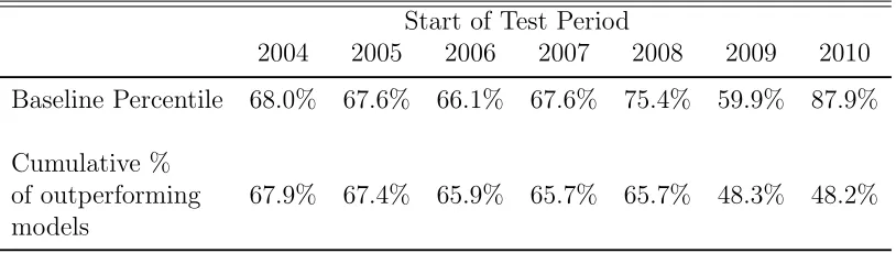
are robust to the choice of test period. Table 3 reports the results of this exercise.

As the test period becomes shorter (moving left to right across rows), the ranking

of the baseline model (lowest RMSFE to highest RMSFE) remains very consistent.

Within each test period, the baseline model is outperformed by 59.9% to 87.9% of all

models.7 _{In addition, the second row highlights the fact that there is a substantial set}

of models that outperform the baseline in all of the test periods. In total, there are

495 models that outperform an AR(1) across every test period we consider. There

is noticeable drop in the percentage of models that outperform the baseline when

the test period starts later than 2009, which is the first test period that excludes the

Great Recession. There are a substantial number of models that forecast relatively

well during the Great Recession, but were mediocre under more normal economic

6

A more complete accounting of these results can be found in Appendix D.

7

conditions.

Table 3: Robustness of Forecasts with Component Revisions

Start of Test Period

2004 2005 2006 2007 2008 2009 2010

Baseline Percentile 68.0% 67.6% 66.1% 67.6% 75.4% 59.9% 87.9%

Cumulative %

of outperforming 67.9% 67.4% 65.9% 65.7% 65.7% 48.3% 48.2% models

From left to right each column increases the estimation period by one year. Column 2 represents our primary estimation period through 2004Q3 with column 3 advancing the estimation period to 2005Q3. Baseline percentile reports the performance of the baseline model relative to all 1024 models (ranked from lowest to highest RMSFE). Row 2 reports the percentage of all models that outperform the baseline model conditional onalso _{outperforming the baseline in all previous test}

periods.

Our results are robust to two other changes. First, the results are robust to

different measures of forecast accuracy. Calculating mean absolute forecast error

(MAFE) in place of RMSFE yields a similar ranking of models.8

We also investigate

the role of outliers in component revisions. In each component revision series there

are one to three large outliers (greater than three standard deviations). Censoring

these outliers at 3 standard deviations actually increases the relative performance

of the component models. After censoring outliers, 69.3% of component-augmented

dynamic regression models outperform the baseline model, up from 67.9% when the

outliers are not censored.

8

3.4

Bayesian Model Comparison

The results above suggest that at least one of our component-augmented models

outperforms the baseline AR(1) model in terms of forecasting accuracy. However,

since we are testing over 1,000 different models, it may not be surprising that at

least one of these models should have outperformed the baseline. Our results above

indicate that a large number of our component-augmented models outperform the

AR(1) model. Additionally, the first revision of consumption appears especially

important, suggesting that this result is being driven by something meaningful. In

this section, we show, in a theoretically rigorous manner, that the superior forecast

performance of component-augmented models is likely not driven by statistical noise.

Using our Bayesian framework outlined in Section 2.1 we find that the probability

of the AR(1) model being the best forecasting model decreases substantially, from

a prior probability of 50% to a posterior probability of only 4.5%. In addition, the

findings in this section reinforce the frequentist results — we find that models that

include the first revision of consumption growth outperform all other models and

that the first revision of consumption growth likely belongs in the forecasting model

for GDP growth.9

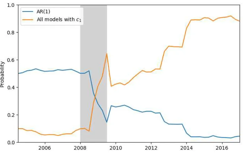
Figure 2 shows the model probabilities for the AR(1) model and the sum of model

probabilities over all models that include the first revision of consumption growth,c1.

Given our priors, since we have 10 variables, there is a prior probability of roughly

10% on the mass of models that includesc1. As time progresses and the probabilities

are revised based on forecast performance, we see a large increase in the posterior

probability of models that include c1. This increase is substantial during the Great 9

Recession, with smaller, but persistent, gains accruing largely between 2010 and

2015. At the last date in the test sample, the models containing c1 accounted for

88.1% of the posterior probability, with the AR(1) model falling from 50% to 4.5%

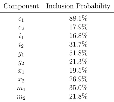
probability over the same horizon. Table 4 provides inclusion probabilities for each

component revision. It again highlights the important role of the first revision to

consumption.

Figure 2: Selected Model Probabilities over Time

The vertical axis reports the posterior probability. As more test sample data accrues, the probability that the best forecasting model includesc1increases while the probability of the AR(1) model being

Table 4: Inclusion Probabilities for Component Revisions

Component Inclusion Probability

c1 88.1%

c2 17.9%

i1 16.8%

i2 31.7%

g1 51.8%

g2 21.3%

x1 19.5%

x2 26.9%

m1 35.0%

m2 21.8%

Inclusion probability for each variable is based on the model probabilities derived using the Bayesian predictive density as of 2017Q1.

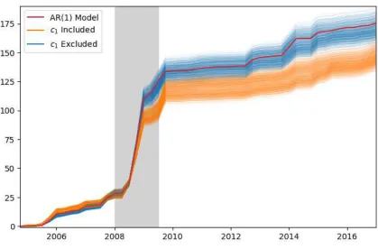
More strikingly, Figure 3 plots the cumulative squared forecast error, where

smaller values indicate superior forecast performance. The point forecasts from

mod-els that include the first revision of consumption generally outperform modmod-els that

exclude it. The baseline model is outperformed by every model in which the first

revision of consumption is present; this is also true for the cumulative sum of the

log posterior density, which is qualitatively similar. Our Bayesian model comparison

underscores, in a statistically rigorous way, that it is highly likely (95.5% probability)

that the best forecasting model in the large set that we consider includes at least

one component revision. Moreover, according to our posterior model probabilities

there is roughly an 88% probability that the best model contains the first revision

to consumption. In combination, these facts imply that we both identify that there

is information pertinent for forecasting in component revisions and that the first

Figure 3: Cumulative Sum of Squared Forecast Error, All Models

The vertical axis is the cumulative sum of squared forecast errors. Smaller values indicate superior point-forecast performance. All models includingc1 outperform the baseline AR(1) model.

4

Conclusion

This paper conducts a real-time forecasting exercise for advance estimates of real

GDP growth where we compare the forecast performance of dynamic regression

mod-els that are augmented with data revisions. Similar to previous work in the literature,

we find no increase in forecast performance using aggregate GDP revisions.

Surpris-ingly, component revisions appear to improve forecast performance with nearly 68%

of such models outperforming an AR(1) model. The best of these models would

baseline.

Without ana priori reason to exclude certain revisions, we consider a large set of

alternative models. Because of this, we conduct an extensive investigation into the

significance of our results. Component-augmented models outperform our baseline

in a variety of test periods, and a large percentage (48%) of component-augmented

models outperform the baseline in all of our seven test periods (2004Q4:2010Q4

advanced in one year increments). We perform Bayesian model comparison to

illus-trate that the increase in forecast performance goes beyond statistical noise. Despite

a 50% prior probability on the AR(1) model, its posterior probability falls to 4.5%.

This implies that there is a 95.5% probability that at least one of the component

revisions belongs in the most accurate forecasting model for the advance estimate of

GDP growth. Finally, we identify the strong role of the first revision to consumption,

c1, in improving forecast performance. Models that include c1 generally outperform

models that exclude it (see Figure 3). Of all the component revisions, c1 has by far

the highest inclusion probability at 88.1%.

On the whole, we feel that the results paint a compelling picture that GDP

component revisions improve forecast accuracy. The most direct implication of this

finding is that some GDP revisions contain information about future GDP growth.

This research suggests several potential paths for future research. While we have

identified the role of consumption, the exact mechanism and the importance of other

components could be a fruitful line of inquiry. Our results may also have important

implications for other strains of the real-time forecasting and data revisions

litera-ture. In particular, there may be implications for the debate surrounding whether

data revisions contain news or noise (e.g. Mankiw and Shapiro (1986)) and the

effi-ciency of government data releases (e.g. Aruoba (2008)). The value of this research

con-tent highlights their pocon-tential importance in a wide array of economic planning and

Bibliography

Amisano, G. and Geweke, J. (2017). Prediction using several macroeconomic models. Review of Economics and Statistics, 99(5):912–925.

Aruoba, S. B. (2008). Data revisions are not well behaved. Journal of Money Credit and Banking, 40(2-3):319–340.

Clements, M. P. and Galv˜ao (2012). Improving real-time estimates of output gaps and inflation trends with multiple-vintage VAR models. Journal of Business and Economic Statistics, 30(4):554–562.

Clements, M. P. and Galv˜ao (2013a). Forecasting with vector autoregressive mod-els of data vintages: US output growth and inflation. International Journal of Forecasting, 29:698–714.

Clements, M. P. and Galv˜ao (2013b). Real-time forecasting of inflation and output growth with autogressive models in the presence of data revisions. Journal of Applied Econometrics, 28:458–477.

Croushore, D. (2006). Forecasting with real-time macroeconomic data. In Elliot, G., Granger, C. W., and Timmermann, A., editors,Handbook of Economic Forecasting, volume 1, pages 961–982. Elsevier, North-Holland.

Croushore, D. (2011). Frontiers of real-time data analysis. Journal of Economic Literature, 49(1):72–100.

Croushore, D. and Stark, T. (2003). A real-time data set for macroeconomists: Does the data vintage matter? Review of Economics and Statistics, 85(3):605–617.

Eklund, J. and Karlsson, S. (2007). Forecast combination and model averaging using predictive measures. Econometric Reviews, 26(2-4):329–363.

Faust, J., Rogers, J., and Wright, J. (2003). Exchange rate forecasting: The errors we’ve really made. Journal of International Economic Review, 60:35–39.

Fixler, D. J., Greenaway-McGrevey, R., and Grimm, B. T. (2011). Revisions to GDP, GDI, and their major components. Survey of Current Business, 91:9–31.

Howrey, E. P. (1978). The use of preliminary data in econometric forecasting.Review of Economics and Statistics, 6(2):193–200.

Kishor, N. and Koenig, E. (2012). VAR estimation and forecasting when data are subject to revision. Journal of Business and Economic Statistics, 30(2):181–190.

Koenig, E. F., Dolmas, S., and Piger, J. (2003). The use and abuse of real-time data in economic forecasting. Review of Economics and Statistics, 85(3):618–628.

Koop, G. (2003). Bayesian Econometrics, chapter 6. Wiley, Chichester, England.

Koop, G. and Potter, S. (2004). Forecasting in dynamic factor models using bayesian model averaging. The Economics Journal, 7(2):550–565.

Mankiw, G. N. and Shapiro, M. D. (1986). News or noise: An analysis of GNP revisions. Survey of Current Business, 66(5):20–25.

Robertson, J. and Tallman, E. (1998). Data vintages and measuring forecast model performance. Federal Reserve Bank of Atlanta Economic Review, Fourth Quarter:4–20.

Sargent, T. (1989). Two models of measurements and the investment accelerator. Journal of Political Economy, 97:251–287.

U.S. Bureau of Economic Analysis (2015). Why does BEA revise GDP esti-mates? Retrieved from https://blog.bea.gov/2015/07/13/why-does-bea-revise-gdp-estimates-2/.

Young, A. H. (1993). Reliability and accuracy of the quarterly estimates of GDP. Survey of Current Business, 73(October):29–43.

Appendix A

Data Construction

Our primary series of interest is the advanced estimate of real GDP growth. We utilize the series directly from the Real-Time Data Set for Macroeconomists, hosted at the Federal Reserve Bank of Philadelphia. For convenience, we outline some of the critical aspects of constructing the data. Interested readers should consult the extensive documentation that accompanies the data set.10 _{The advanced estimate}

of annualized quarter over quarter GDP growth is constructed as

y_tT =

"

Y_tT YT

t−1

4

−1

#

×100, (5)

where T represents the first vintage that contains an observation of t. For our purposes the difference betweenT and twill always correspond to about 1 month or the release lag from the end of a quarter until the advance release of real GDP. A more concrete example is shown below:

y19911992Qm41 =





Y1992m1 1991Q4

Y1992m1 1991Q3

!4

−1



×100, (6)

wherey1992m1

1991Q4 would be the advance estimate of real GDP growth for 1991Q4 based on

the vintage released in January 1992. We calculate revisions to GDP as the difference in growth rates between monthly releases fort. Therefore, the first revision r1 is the

difference between growth rates for the first (T) and second (T+ 1) releases of period

t GDP growth:

r1,t =ytT+1−y T

t. (7)

The second revision then is:

r2,t =ytT+2−yT

+1

t . (8)

We omit the vintage superscript and time subscripts from revisions for clarity. It is understood that first revisions can only exist after a second vintage containingt has been released. Its superscript is therefore T + 1 and the second revision’s is T + 2. Typically level changes in GDP due to definitions and measurement occur in ad-vance releases. Since our growth rates are calculated within vintages and subsequent revisions (i.e. second and third) use the same definitions as the advance release, we

10

do not make any additional changes to our data to account for revisions beyond the advance, second, and third releases.

Our component data for real personal consumption expenditures, real exports of goods and services, real imports of goods and services, and real government consump-tion and gross investment are also directly from the Philadelphia Federal Reserve’s Real-Time Data Set for Macroeconomists. Our data for component revisions is con-structed in the same way as for revisions to GDP. For example, letC be the level of consumption in GDP (measured in real terms), then the annualized growth rate of

C is:

cT_t =

"

CT t

CT t−1

4

−1

#

×100. (9)

The data we use for estimation are the first and second revisions to c, which are again measured as differences in consumption growth:

c1,t =cTt+1−c T

t. (10)

The second revision then is:

c2,t=cTt+2−cT

+1

t . (11)

As with the aggregate revisions, we drop the vintage superscript and time subscripts in order to refer to revisions generally. We also tolerate the abuse of notion (using

c for revisions and growth) in order to present a simpler composition in the text. The notation for government spending, investment, import, and export expenditures follow an identical construction and are designatedg, i, m, andx, respectively.

Appendix B

Summary Statistics

Table 5 provides summary statistics for the advance estimates of real GDP growth. It begins in 1991Q4 to coincide with the BEA’s change from GNP to GDP as its primary measure of output. Of our 101 observations, we withhold 50 for out-of-sample comparisons between models. The single gap in our out-of-sample stems from the lack of an advance release of real GDP in 1995Q4.11 _{For comparison, the post-war}

(1947Q2:2017Q1) real GDP growth rate, using the most recent vintage (September 28th, 2017), is 3.22% with a standard deviation of 3.91%.

Table 5: Advance Estimates of Real GDP Growth

Period Dates N Mean Std. Dev. Gaps

Full Sample 1991Q4 - 2017Q1 101 2.51% 1.95% 1 Estimation Sample 1991Q4 - 2004Q3 51 3.13% 1.74% 1 Test Sample 2004Q3 - 2017Q1 50 1.88% 1.97% 0

We also utilize the differences in growth rates between advance and second es-timates (first revision) and second and third eses-timates (second revision). Summary statistics for these revisions are presented in Table 6. As has been documented by others, the first revision to GDP and GDP growth tends to be much larger than the second revision (roughly 6 times larger in our full sample).12

However, the differ-ence between first and second revisions is considerably lower in the second half of our sample (27 times larger vs. 2 times larger). There is also a greater variance in first revisions than second revisions. Our revision data has an additional gap (be-yond what was presented in Table 5) resulting from a missing second release of GDP growth in 2003Q3.

11

For greater explanation on these types of data eccentricities see the extensive documentation that accompanies each series in the Real-Time Data Set for Macroeconomists.

12

Table 6: Revisions to Real GDP Growth

Mean Std. Dev. Gaps

Period r1 r2 r1 r2 r1 r2

Full Sample 0.129% 0.022% 0.641% 0.370% 2 1 Estimation Sample 0.191% 0.007% 0.591% 0.313% 2 1 Test Sample 0.068% 0.038% 0.688% 0.424% 0 0

r1 andr2refer to the first and second revisions to real GDP growth, respectively.

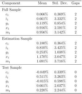
Table 7: First Revisions to GDP Components

Component Mean Std. Dev. Gaps

Full Sample

c1 0.066% 0.369% 2

i1 0.661% 3.332% 2

g1 0.119% 0.854% 2

x1 0.916% 2.591% 2

m1 0.956% 3.142% 2

Estimation Sample

c1 0.180% 0.364% 2

i1 0.810% 3.425% 2

g1 0.253% 1.038% 2

x1 1.170% 3.047% 2

m1 1.691% 3.716% 2

Test Sample

c1 -0.049% 0.339% 0

i1 0.511% 3.263% 0

g1 -0.015% 0.598% 0

x1 0.661% 2.037% 0

m1 0.220% 2.244% 0

Table 8: Second Revisions to GDP Components (rk,2)

Component Mean Std. Dev. Gaps

Full Sample

c2 0.014% 0.358% 1

i2 -0.001% 1.415% 1

g2 -0.075% 0.475% 1

x2 0.127% 1.389% 1

m2 -0.126% 1.486% 1

Estimation Sample

c2 0.039% 0.236% 1

i2 -0.081% 1.433% 1

g2 -0.181% 0.595% 1

x2 0.068% 1.424% 1

m2 -0.215% 1.744% 1

Test Sample

c2 -0.012% 0.451% 0

i2 0.081% 1.405% 0

g2 0.032% 0.276% 0

x2 0.187% 1.365% 0

m2 -0.035% 1.179% 0

Appendix C

Coefficient Priors

In addition to the model priors, each particular model has priors on the regression coefficients and the AR(1) term in the error equation. For each model, we place priors on the regression coefficients, βr, and the AR(1) term, ρr. For the k × 1

vector of regression coefficients,βk, in model r, we follow convention and setp(βr) =

N(0, Vr). Our prior is that each regressor has no effect, with the tightness of that

belief controlled by the covariance matrix, Vr. Put another way, our prior is that

past revisions to GDP growth do not contain information important to forecasting future GDP growth.

Since we are considering a large set of models, we set these priors in an automatic fashion. Our prior belief is that each coefficient is independent, so all non-diagonal elements ofVr are zero. We assume that each coefficient is given as:

p(β_rk) =N(0, σ_β2)

σ_β2 = 1

whereβk

r is the coefficient corresponding to the k

th _{regressor in model r.}

For the AR(1) term, ρr, we set:

p(ρr) =N(0.5, σρ2)

σ2_ρ = 0.52

Appendix D

Additional Results

Table 9: Forecasting with Component Revisions

Component Outperforming Models Performance of models with component (%) with component (%)

c1 73.7% 100%

g1 59.3% 80.5%

i2 53.4% 72.5%

m2 52.8% 71.7%

x1 51.1% 69.3%

x2 50.1% 68.0%

m1 46.6% 63.3%

g2 46.0% 62.5%

c2 45.6% 61.9%

i1 43.9% 59.6%