Munich Personal RePEc Archive
Resale Price Maintenance with Strategic
Customers
Bazhanov, Andrei and Levin, Yuri and Nediak, Mikhail
Smith School of Business, Queen’s University, Kingston, ON,
Canada
27 May 2017
Online at
https://mpra.ub.uni-muenchen.de/79467/
Resale Price Maintenance with Strategic Customers
Andrei Bazhanov, Yuri Levin and Mikhail Nediak
Smith School of Business, Queen’s University, Kingston, ON, K7L3N6, Canada
Abstract: We consider a decentralized supply chain (DSC) under resale price maintenance (RPM)
selling a limited-lifetime product to forward-looking customers with heterogeneous valuations.
When customers do not know the inventory level, double marginalization in DSC leads to a higher
profit and lower aggregate welfare than in centralized supply chain (CSC). When customers know
the inventory, DSC coincides with CSC. Thus, overestimation of customer awareness may lead
to overcentralization of supply chains with profit loss comparable with the loss from strategic
customers. The case with unknown inventory is extended to an arbitrary number of retailers
with inventory-independent and inventory-dependent demand. In both cases, the manufacturer,
by setting a higher wholesale price, mitigates the inventory-increasing effect of competition and
reaches the same profit as with a single retailer. The high viability of RPM as a
strategic-behavior-mitigating tool may serve as another explanation of why manufacturers may prefer DSC with RPM
to a vertically integrated firm.
Keywords: limited-lifetime product, strategic customers, limited information, aggregate welfare,
1
Introduction
Resale price maintenance (RPM) is any of a variety of practices through which manufacturers
restrict resellers in the prices that they may charge for the manufacturer’s products. RPM can be
imposed explicitly as a manufacturer’s suggested retail price (MSRP or list price) or as a price floor
(minimum RPM), or the price can be set implicitly by, for example, fixing the retailer margin, see
European Commission (2010). The legal status and use of RPM has been controversial for over
a century, and evidence suggests that both the scale of RPM use and the effects on the economy
are underestimated. Overstreet (1983) provides an extensive review of RPM use for the period
when this practice was per se legal. In 1988, when RPM was illegal in the USA, the Supreme
Court adopted a wide use of the Colgate doctrine according to which a manufacturer may refuse
to deal with a retailer if it does not comply with the manufacturer’s price policy. Butz (1996)
quoted antitrust authorities arguing that RPM became “ubiquitous” and “endemic”, “but based
upon ‘winks and nods’ rather than written agreements that could be used in court.”
RPM attracted growing attention after a 2007 Supreme Court declaration that
manufacturer-imposed vertical price fixing should be evaluated using a rule of reason approach. MacKay and
Smith (2014) provide explicit evidence of RPM and comment that the firms involved in this practice
“include manufacturers and suppliers of childcare and maternity gear, light fixtures and home
accessories, pet food and supplies, and rental cars. Sony has publicly used minimum RPM on
electronics such as camcorders and video game consoles, and as of mid-2012, Sony and Samsung
began enforcing minimum RPM on their televisions. Other retailers do not comment on whether or
not they enter minimum RPM agreements, perhaps due to negative consumer sentiment associated
with higher prices.”
Manufacturers of various goods including electronic devices and seasonal goods repeatedly
intro-duce new versions of their products. The rapid pace of fashion, innovations, and change of seasons
limit the lifetime of these versions, reducing customer valuations in time. As a result, such products
may regularly appear on clearance sales. According to the National Retail Federation, the practice
of markdown pricing has followed a growing trend since 1960’s (Deneckere et al. (1997) ). When
product value is relatively durable, retailers may markdown in order to price-discriminate among
de-mand even when the dede-mand can be predicted with a high accuracy. This may happen when sales
at the list price increase with the quantity of the product exposed to customers, see, for example,
Urban (2005).
Customers accustomed to markdown pricing form expectations about future clearance sales and,
using these expectations, may engage in forward-looking or patient shopping behavior by delaying
the purchase until price reduction. The time of discount can be easily anticipated for seasonal
goods, and the size of the discount is usually predictable because it is often product specific and
expressed in round numbers (20% off, 50% off, etc.). Customers realize that delaying the purchase
may reduce the sense of novelty and their enjoyment of the product, but they still make this
intertemporal trade-off. Since forward-looking behavior is an instance of strategic behavior and we
do not consider other forms of this behavior, we use these terms as synonyms.
Starting from Coase (1972), theoretical and empirical studies confirm that strategic customer
behavior hurts sellers and may reduce profit up to 50%, see, for example, a comprehensive review
in G¨onsch et al. (2013). Coase conjectured that a monopolistic seller of a durable good with a
secondary market is not able to extract monopolistic profit when strategic customers know the
total amount of the product and total demand. Even the customers with high valuations of the
product may wait until the price is reduced to the competitive level because the seller has an
incentive to sell the product in small portions reducing the price with time in order to capture
customer surplus. Such “price skimming” decreases the market value of the product for the first
buyers, and they may end up with a negative surplus. Due to the customer delays, the profit from
skimming may be significantly lower than a monopolistic profit from a one-time sale of a portion
of available product. However, the seller cannot credibly commit to the one-time sale because
customers know that the seller may have extra profit by selling an additional product after this
sale is realized. This phenomenon is referred to as “dynamic inconsistency.”
Despite broad evidence of the negative effects for sellers, Desai et al. (2004), Arya and Mittendorf
(2006), and Su and Zhang (2008) prove that when customers are strategic, a decentralized supply
chain (DSC) may enjoy a higher total profit than that of the centralized supply chain (CSC). These
studies show that the Coase problem may be solved by adding an intermediary retailer. The benefit
results from double marginalization, which, without strategic customers, leads to suboptimally low
unit cost. This effect provides a credible commitment of the SC to a high retail price or low
quantity, which cannot be achieved for a centralized production-selling unit under the Coase setup.
Our paper complements these studies by showing that DSC with strategic customers may have
a higher profit than CSC even when the seller does not suffer from the Coase problem in its extreme
case, that is, when the secondary market can be neglected, making possible intertemporal price
discrimination, see, for example, Bulow (1982). Under price discrimination, the two-period profit
of CSC is higher than the profit if sales occur only in the first period despite the negative effect of
customer delays. This situation means that the seller does not need to commit to first-period sales.
In other words, even when CSC does not suffer from dynamic inconsistency, DSC may perform
better due to double marginalization, which, in this case, permits higher prices.
We derive this result in a two-period model for a limited-lifetime product, a contract with
RPM for DSC, and forward-looking customers with heterogeneous valuations who do not know the
retailer’s inventory level. In reality, customers often do not know inventories or may ignore this
information even when it is available. Comparison with the case of known inventory yields the value
of information disclosure or, alternatively, the value of overestimation of customers’ reaction to this
information. There are a many contracts that include RPM. In this paper we restrict attention to
contracts with a two-part tariff where the manufacturer sets both the retail price and the wholesale
price and a fixed (franchise) fee. This follows, for example, the work of Rey and Tirole (1986),
Gal-Or (1991),§5.2 of Gurnani and Xu (2006), and Rey and Verg´e (2010).
Our analysis is distinct from those in the above studies because our focus is on the intertemporal
effects of strategic customers and limited life of the product. In particular, the retailer may sell
the product in both periods but must procure the total two-period inventory in the first period,
given the inputs from the manufacturer. The manufacturer solves a one-period problem because
the product is not produced in the second period. As a result, we do not use subgame perfect
equilibrium as do Desai et al. (2004) and Arya and Mittendorf (2006) who consider SC under
two-part tariffs and wholesale price contracts respectively. In terms of the equilibrium concept, our
setup is closer to that of Su and Zhang (2008) who use rational expectations equilibrium (REE)
for the wholesale price, buyback, sales rebates, and markdown money contracts.
Another flexibility for the retailer in our setup is that the second-period price is not fixed
clearing. Besides the growing empirical evidence on markdowns mentioned above, this assumption is
consistent, for example, with the sales of copyrighted materials in Japan where retailers are selling
first at MSRP and eventually “reducing prices for consumers who don’t mind waiting a while
before they buy”; see Nippop (2005). Similarly to Desai et al. (2004) and Arya and Mittendorf
(2006), we consider deterministic demand in order to have a more tractable problem. Fisher and
Raman (1996) shows that demand uncertainty in the fashion apparel industry can be significantly
reduced by analyzing preliminary sales of the product. The effects of uncertainty are considered,
for example, in Su and Zhang (2008) and Cachon and Swinney (2009).
In this framework, DSC sets prices higher and inventory lower than CSC, which is a usual effect
of double marginalization. This known effect leads to an interesting result in our setup. When
customers exhibit higher levels of strategic behavior (to be defined), more customers delay their
purchases under CSC, which is a usual consequence of forward-looking behavior. For DSC, the
number of waiting customers decreases because more strategic customers pay more attention to
the expected second-period price, which is higher under DSC. As a result, DSC enjoys more sales
in the first period at a higher price than CSC. This comparative increase in the first-period profit
outweighs a relative loss in the second-period sales.
A frequent motivation for studying RPM is the welfare effect of this policy. We show that
RPM, compared to CSC, improves neither customer surplus nor aggregate welfare. However, it is
questionable that RPM is the primary culprit in these losses for two reasons. First, some customers
with low valuations suffer from the strategic behavior of other customers with higher valuations
even when the first-period price is fixed (no manufacturer decisions). Second, CSC can reach the
same profit and hurt welfare in the same way as RPM simply by disclosing inventory information to
the customers. Therefore, under DSC with known inventory, manufacturer “turns off” unnecessary
double marginalization by setting the wholesale price equal to unit cost. The result implies, first,
that strategic customer behavior itself may be a fundamental reason of welfare losses; and second,
that overestimation of customer knowledge of inventory or underestimation of strategic customer
behavior may lead to overcentralization of SC. We show that profit loss from this overcentralization
may be comparable with the loss from strategic customers.
We present a review of related literature in §2, describe a general model and provide a
arbitrary number of retailers are considered in §4, and the conclusions are in §5. All proofs and
supplementary materials are in the online appendix.
2
Literature review
The negative effect of double marginalization has been known since Spengler (1950) who shows in
a model with linear deterministic demand that “both the consumers and the firm benefit” from
vertical integration, that is, when all production-selling decisions comply with a single criterion. A
broad literature on SC coordination, reviewed in Cachon (2003), examines the abilities of various
contracts to reach the same profit as CSC. These results raise a question: Why do decentralized
supply chains exist if their profits never exceed the one of CSC? The reasons include legal issues
that motivated the work of Spengler or prohibitively high costs of CSC construction for small firms.
The works of Desai et al. (2004), Arya and Mittendorf (2006), and Su and Zhang (2008) reviewed
in Su and Zhang (2009), provide one more reason: double marginalization can lead to a strictly
greater profit of DSC than that of CSC when it serves as a commitment device to higher prices or
low inventories while customers strategically delay their purchases. The current paper extends this
line of research by showing that when customers are strategic, DSC under RPM outperforms CSC
even without secondary markets and with competing retailers.
The study of strategic buyers starts from the famous conjecture of Coase (1972), which is
formally supported in subsequent work, for example, by Bulow (1982). These early findings have
led to further research in the context of intertemporal pricing, which is systematically reviewed in
G¨onsch et al. (2013). In particular, Liu and van Ryzin (2008) concur that “capacity decisions can
be even more important than price in terms of influencing strategic customer behavior”; they study
the effects of capacity decisions when prices are fixed while customers have full information and
can be risk-averse. Liu and van Ryzin find that capacity rationing can mitigate strategic customer
behavior but is not profitable when customers are risk neutral. Under competition, which typically
increases market supply, the effectiveness of capacity rationing is reduced, and there exists a critical
number of firms beyond which rationing never occurs in equilibrium. Further development of this
work by Huang and Liu (2015) shows that capacity rationing is also less effective under inaccurate
Unlike Liu and van Ryzin (2008), we consider retailers’ capacity decisions in a SC framework
when the manufacturer uses RPM and optimally sets the first-period price. Following Liu and van
Ryzin (2008), we check the robustness of RPM as a low-inventory-commitment tool with respect to
the number of retailers. First, similarly to Liu and van Ryzin (2008), we consider equal allocation
of the first-period demand among the retailers. Then we raise the bar by extending the test to
inventory-dependent demand when the first-period sales increase in retailers’ inventories, which, in
addition to competition, further boosts the supply.1 The possibility of salvage sales, included in the
case of inventory-dependent demand, further increases retailers inventories. In response to these
challenges, the manufacturer raises the wholesale price, thereby achieving a desirable inventory
level and profit of DSC that exceeds the one of CSC for any number of competing retailers. These
extensions confirm the high viability of RPM as a strategic-behavior-mitigating tool, which may
serve as another explanation of why manufacturers may prefer RPM to a vertically integrated firm.
A review of the theories explaining the existence of RPM is provided in Orbach (2008). In
particular, RPM can be welfare-reducing when it leads to retailer cartels. In other cases, RPM can
be welfare-improving, for example, when the manufacturer uses it to protect the appeal of branded
products against using them as loss leaders or supports the retailers providing costly
demand-increasing services against free riders that capture the demand by cutting the price. These theories
do not consider the effects of strategic customers. Other contracts with RPM considered in the
literature presume, for example, that manufacturer, besides retail price, fixes the quantity of the
product, procured by the retailer, see, for example, Mukhopadhyay et al. (2009). In our setting,
this assumption would lead to a passive retailer without double marginalization, which is a crucial
effect to increase the profit of SC when customers are strategic. A review of other vertical restraints
can be found in Lafontaine and Slade (2013).
3
RPM with one retailer
We consider a two-period market where a manufacturer sells a limited-lifetime product either
directly to customers (CSC) or via an intermediary retailer (DSC). Following Desai et al. (2004)
and Arya and Mittendorf (2006), we assume that the manufacturer and retailer know the demand
period and, therefore, there is no secondary market. The manufacturer and retailer do not offer
the product for rent due to high remarketing costs or legal issues, see, for example, Bulow (1982).
3.1 Model description and general results
Under CSC, the manufacturer chooses the first-period price p1 and inventory Y. By choosing Y,
the manufacturer chooses either one-period or two-period sales depending on the profitability of
price-discrimination compared to the first-period sales only. If Y > D, the second-period price p2
is determined by marked clearing. Following Arya and Mittendorf (2006), who adopt a basic setup
from Bulow (1982), we normalize the manufacturer’s cost to zero, and then the profit of CSC is
ΠC =p1min{Y, D}+p2(Y)(Y −D)+, (1)
where superscript “C” means CSC.
Under DSC, the manufacturer maximizes its profit by offering a contract with RPM at the
be-ginning of the first period. Since the product is not produced in the second period, the manufacturer
faces a one-period problem. Following Desai et al. (2004), we disregard other retailer costs except
the wholesale pricew.We will call an RPM contract a tuple (p1, w, F), wherep1 is the first-period
retail price or MSRP and F is a fixed fee. Equivalently, RPM can be determined by (p1, mr, F),
where mr = (p1−w)/p1 is a retailer margin. According to the studies of SC contracts with fixed
fee, for example, Rey and Tirole (1986) and Gurnani and Xu (2006), the manufacturer setsF that
makes the retailer indifferent between accepting and rejecting the contract. When demand is
de-terministic, the retailer accepts any contract with nonnegative profit; otherwise, the manufacturer
may not supply the product leading to zero retailer profit. Therefore, F equals retailer profit and
the manufacturer total profit equals the profit of DSC. Henceforth, we denote this profit ΠD and
the manufacturer and retailer parts of this profit Πmand Πrrespectively. In practice, the difference
F−Πr is a positive constant, which does not affect the results below.
Retailer maximizes its profit by selecting the initial inventory level Y, which may lead either
to one- or two-period sales. In the latter case, the second-period price is determined by market
clearing. Then the manufacturer and retailer parts of DSC profit are
Πm = wY, (2)
Customers, similarly to Desai et al. (2004), arrive at the start of the first period and their
valuationsvare uniformly distributed on the interval [0,1]. We normalize the number of customers
to one, that is, the potential demand in the first-period is 1−p1. Normalization effectively
ex-presses revenue and inventory as “unitless” quantities and the first-period price p1 as a share of
the maximum valuation implying p1 ≤ 1. The demand 1−p1 is “potential” because it includes
all customers with valuations not less than p1.We show below that when some of the customers
strategically delay their purchases, the actual first-period demand isD= 1−vmin<1−p1,where
vminis the valuation of a customer who is indifferent between buying in the first period or waiting.
Then, a general expression for a seller profit with a unit cost cbecomes
Π =−cY +p1min{Y,1−vmin}+p2(Y)(Y −1 +vmin)+, (4)
wherec= 0 for CSC andc=w= (1−mr)p1 for the retailer in DSC. Note that profit (4) increases
linearly inY when Y ≤1−vmin =D. Therefore, the inventory of a profit-maximizing firm is not
less than D, that is, there are no stockouts, implying that the first-period sales equal D and the
second-period inventory is Y −D=Y −(1−vmin).
A decrease in valuations, similarly to Desai et al. (2004), is captured by factor β ∈[0,1]: if the
customer’s first-period valuation isv, the second-period valuation isβv. Suppose the second-period
inventory Y −1 +vmin > 0. The number of customers remaining in the market is vmin and the
maximum second-period valuation isβvmin. Therefore, the market clearing condition for the second
period takes the form vminβvmin−p2
βvmin =Y −1 +vmin, or, equivalently,
p2 =β(1−Y). (5)
We use a logical restrictionβ > c,which guarantees that the highest-valuation customer is prepared
to pay more than the unit cost in the second period. If this restriction does not hold, the clearance
price can never be above the unit cost. This second-period setup differs from Desai et al. (2004)
and Arya and Mittendorf (2006) where the product is produced in both periods, a seller chooses
quantities to sell in both periods, and there is second-period used-product market. The setup differs
also from Su and Zhang (2008) where the second-period price is exogenously fixed. The following
assumption is common for all cases considered in this paper.
the second-period surplus discount factorρ∈[0,1). Customers are non-cooperative and do not know
total demand.
Undervaluation of the surplus from delaying a purchase, similarly to Desai et al. (2004), means
that even for a product that does not depreciate much by the second period (β is near one),
customers with any valuation may myopically ignore the second period during the first-period
deliberations, which is captured byρ = 0. The value ofρ may depend on the market targeted by
the product, for example, for age- or culture-oriented products, and on the customer confidence
in the stability of the financial situation. Customers with a higher ρ place more emphasis on the
second period in their wait-or-buy decisions. Thus, unlike β, which models an objective decrease
in valuations, the customer’s discount factor ρ is a subjective parameter describing the level of
strategic behavior. The essence of the distinct roles of β and ρ has been succinctly captured
by Pigou (1932): “Everybody prefers present [that is, ρ < 1] pleasures or satisfaction of given
magnitude to future pleasures and satisfaction of equal magnitude [that is,β = 1], even when the
latter are perfectly certain to occur.” Frederick et al. (2002) provide a review of empirical estimates
of customers’ discount rates.
Similarly to Desai et al. (2004), customers are homogeneous in ρ and β. This assumption is
applicable to any products targeting specific market segments. Some empirical studies, for example,
Hausman (1979), claim a dependence of the discount rate on income (which serves sometimes as a
proxy for product valuation). Other studies, however, show that the discount rate does not vary
significantly with income, see, for example, Houston (1983). We do not include ρ = 1 because
the case ρβ = 1 needs a special analysis increasing the volume of the paper. When this case is
interesting, it is considered as a limiting case asρβ→1. Note also, that we do not useρto calculate
the actual (realized) total customer surplus (§3.3) sinceρmodels only customer first-period buying
behavior. However, we do use β for this goal because deterioration of the product value indeed
decreases the realized second-period surplus.
Subsections below compare the cases where customers know and do not know the inventory level.
A general sequence of events for CSC in both cases is as follows: (a) manufacturer, anticipating
strategic customer behavior, choosesp1andY; (b) the first-period demandDand sales are realized;
(c) the remaining inventoryY −D is cleared at p2.
inventory response to manufacturer decisions and customers’ behavior, offers the contract with
RPM; (b) the first-period demand Dis realized; (c) the retailer accepts the contract and procures
inventory Y; (d) the first-period sales are realized; (e) the remaining inventory Y −D is cleared;
(f) the retailer pays fixed fee to the manufacturer. When customers know the inventory, the
only difference in this sequence is that the first-period demand is realized after retailer’s inventory
decision.
3.2 Customers do not know inventory level
The availability of information about total supply of the product varies among the markets. Some
markets, such as land or real estate, have nearly perfect information, the assumption used, for
example, in Desai et al. (2004), Arya and Mittendorf (2006), and Liu and van Ryzin (2008). In many
other markets, total system-wide inventory is unobservable, which reduces the ability of retailers
to use rationing as a tool for stimulating first-period demand from strategic customers. When
customers do not observe total supply, the problem can be solved by assuming that a seller (either
centralized or a retailer in DSC) preannounces the second-period product availability α ∈ {0,1}
and the price p2, see, for example, Yin et al. (2009). Equivalently, like in Su and Zhang (2008),
it can be assumed that customer expectations of these values are rational, which means that they
coincide with the actual values that will be realized. Both approaches to the information aboutα
andp2 imply that all customers share the same values of these parameters. We stick to the second
(expectations) approach in this section and, therefore, refer to the resulting outcomes as Rational
Expectation Equilibria (REE).
Assumption 2. Customers do not know total product supply but know seller’s cost c and have
expectations of product availability in the second period α¯∈ {0,1} and second-period price p¯2.
Despite knowledge of c,customers cannot infer inventory level because they do not know total
demand. Given expectations ¯α and ¯p2, customers decide whether a first or second-period purchase
maximizes their surplus, which is similar to Su and Zhang (2008)2 or Cachon and Swinney (2009):
Assumption 3. When the product is available, a customer with valuationvbuys in the first period
if and only if (iff ) the first-period surplus σ1 ,v−p1 is not less than the expected second-period
Customers do not consider rationing risk in the first period because there are no first-period
stockouts due to deterministic demand and profit-maximizing firms. Since ¯σ2≥0, customers with
v < p1 never buy in the first period because such a purchase would result in a negative surplus.
For the same reason, customers withβv < p2 do not buy in the second period whenp2 is realized.
The lemma below describes the first-period demand.
Lemma 1. Given customer expectations, surplus-maximizing behavior is to buy in the first period
if v≥vmin, where the unique valuation threshold is given by vmin = maxnp1, min
n
p1−¯αρp¯2 1−¯αρβ , 1
oo
.
The resulting first-period demand is D= 1−vmin.
Based on this lemma and the above assumptions, the retailer profit in DSC is Πr= Πr(Y, p1, w,p2,¯ α¯),
wherep1, w,p¯2,and ¯αare the parameters, and we specifyREE in pure strategies for DSC as follows:
(1) Given p1 and wfrom the manufacturer and customer expectations, let the best response of
the retailer be BR(p1, w,p¯2,α¯) = arg maxY Πr(Y, p1, w,p¯2,α¯).
(2) The tuplehYˆ(p1, w),p2ˆ (p1, w),αˆ(p1, w)iis a REE for givenp1, wiff ˆY(p1, w) =BR(p1, w,p2,ˆ αˆ),
ˆ
p2(p1, w) =β
h
1−Yˆ(p1, w)
i
, and either ˆα(p1, w) = 0 if ˆY(p1, w) = 1−vˆ(p1, w) or ˆα(p1, w) = 1 if ˆ
Y(p1, w)>1−ˆv(p1, w) where ˆv(p1, w) is the equilibrium value ofvmin.
(3) The tuple (F∗, p∗1, w∗, Y∗, p2∗, α∗) is a REE for DSC-profit-maximizing p1 and w iff F∗ =
Πr∗ = Πr(Y∗, p∗1, w∗, p∗2, α∗),where (p∗1, w∗) = arg maxp1,wΠD(p1, w), Y∗ = ˆY(p∗1, w∗), p∗2 = ˆp2(p∗1, w∗), and α∗ = ˆα(p∗
1, w∗).
Similar to Desai et al. (2004), we are interested in market situations when there are sales
in both periods, but, for theoretical completeness, we consider all outcomes in order to provide
the conditions when both-period sales are endogenously determined by market participants. The
following lemma offers these conditions for given unit cost c and p1. This result is used below for
CSC withc= 0 and for the retailer in DSC with c=w= (1−mr)p1.
Lemma 2. A unique REE for given p1 and c with the stated structure exists iff the respective
conditions hold:
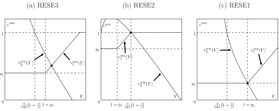
REE1 (First-period sales): vˆ = p1,αˆ = 0,Yˆ = 1−p1, and Π = (ˆ p1 −c)(1−p1) under
condition p1≤c/β.
REE2 (Second-period sales): vˆ= 1,αˆ= 1,pˆ2 = 12(β+c),Yˆ = 12(1−c/β),and Π =ˆ (β−c) 2 4β
REE3 (Two-period sales): ˆv = 2p1−ρc
2−ρβ (increases in ρ), αˆ = 1, pˆ2 = 12(βvˆ+c),Yˆ = 1−12(ˆv+c/β), andΠ =ˆ −cYˆ +p1(1−ˆv) + ˆp2( ˆY −1 + ˆv) under condition βc < p1 <1−ρ2(β−c).
This lemma implies that, for CSC withc= 0 and anyp1 >0,REE1 does not exist, which means
that the second-period sales are always attractive for a vertically integrated seller. The existence
of equilibria in other cases depends on endogenization ofp1 and shown in the proposition below.
Proposition 1. When customers do not know the inventory, there exists only REE3 for both CSC
and DSC. The equilibrium values provided in Table 1 are such that pD1∗ ≥pC1∗, YD∗ ≤YC∗, pD2∗ ≥
pC∗
2 , vD∗ ≤vC∗, and the performance of DSC is ηΠ,ΠD∗/ΠC∗ = 1 + ρ
2β[β2+(2−ρβ)(2−ρβ−2β)] (2−ρβ)2[4−β(1+ρ)2] ≥1.
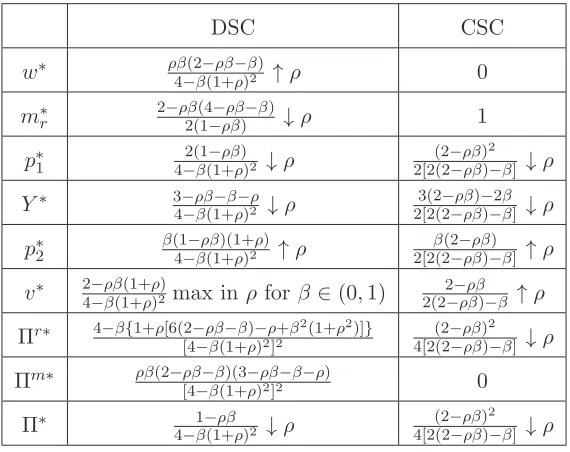
[image:14.612.164.449.325.551.2]All inequalities hold as equalities only atρ= 0 and ρβ→1.
Table 1: Decentralized and centralized SC under incomplete information
DSC CSC
w∗ ρβ(2−ρβ−β)
4−β(1+ρ)2 ↑ρ 0 m∗
r 2−ρβ2(1−(4−ρβρβ)−β) ↓ρ 1 p∗
1 4−2(1−β(1+ρβρ))2 ↓ρ
(2−ρβ)2 2[2(2−ρβ)−β] ↓ρ Y∗ 3−4−ρββ(1+−βρ−)2ρ↓ρ
3(2−ρβ)−2β 2[2(2−ρβ)−β] ↓ρ p2∗ β(1−4−βρβ(1+)(1+ρ)2ρ) ↑ρ
β(2−ρβ) 2[2(2−ρβ)−β] ↑ρ v∗ 2−4−ρββ(1+(1+ρρ)2)max inρ forβ ∈(0,1) 2(2−2−ρβρβ)−β ↑ρ
Πr∗ 4−β{1+ρ[6(2−[4−ρββ(1+−βρ)−)2ρ]2+β2(1+ρ2)]}
(2−ρβ)2 4[2(2−ρβ)−β] ↓ρ Πm∗ ρβ(2−[4−ρβ−ββ(1+)(3−ρ)ρβ2]2−β−ρ) 0
Π∗ 4−1−β(1+ρβρ)2 ↓ρ
(2−ρβ)2 4[2(2−ρβ)−β] ↓ρ
It is known since Mathewson and Winter (1984) that RPM coordinates DSC (the profit of DSC
equals the one of CSC) even with two decision variables. Proposition 1 confirms this result in a
different setting, first, for myopic customers and, second, for ρβ→ 1.In both cases, decentralized
and vertically integrated firms are identical, that is, RPM indeed removes double marginalization.
The case ρβ → 1 deserves a special attention because it also yields ηΠ → 1, which means that
the superiority of RPM over CSC cannot be shown for durable goods only (β = 1) and strategic
whenρβ →1 follows from the elimination of the intertemporal effects since the product is durable
(β = 1) and customers do not distinguish the surpluses from the first- and second-period sales.
Proposition 1 is of a particular interest because previous studies, reviewed in Su and Zhang
(2009), discovered that DSC may outperform CSC only when the latter cannot achieve its highest
profit due to the lack of low-inventory commitment and inexistence of the first-best equilibrium. We
consider a setup where CSC does not suffer from dynamic inconsistency and attains its best profit
in the equilibrium REE3 with sales in both periods. However, DSC performs even better when
customer discount factor is not zero. This result contributes one more explanation to the reasons
why manufacturers may prefer RPM over vertical integration when customers are forward-looking.
It is easy to show that the superiority of DSC arises from double marginalization, which
manu-facturer “turns on” to mitigate strategic delays when customers are not myopic. Indeed, according
to Proposition 1, DSC-pricesp∗
1 and p∗2 are higher and inventory is smaller than for CSC, which is a known effect of double marginalization. The higher ρ, the more customers delay their purchases
under CSC (v∗ increases in ρ), which is a known effect of strategic behavior. Meanwhile, under
DSC, the number of waiting customers is always less than for CSC (vD∗ < vC∗ forρ ∈(0,1)) and
may even decrease inρforβ <1.This occurs because customers with higherρ pay more attention
on the expected second-period price, which is higher under DSC. As a result, DSC enjoys more
first-period sales at a higher price than CSC. As Proposition 1 shows, this comparative increase in
the first-period profit exceeds a relative loss in the second-period sales.
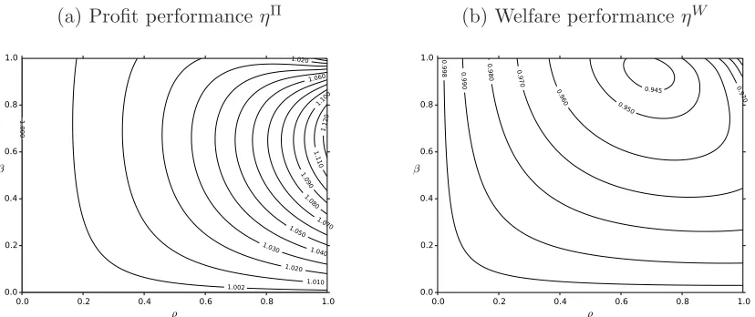
A value of decentralizationcan be estimated by the relative difference
ΠD∗−ΠC∗
/ΠC∗
|ρ→1= β(1−β)
(2−β)2. A unique maximizer βmax = 2/3 leads to maxβ
ΠD∗−ΠC∗
/ΠC∗
|ρ→1 = 1/8, that is,
when customers are strategic and do not know the inventory, RPM can improve supply chain profit
up to 12.5% (Figure 1 (a)). For comparison, the loss of CSC profit due to strategic customers at
βmaxis ΠC∗|
ρ=0−ΠC∗|ρ→1/ΠC∗|ρ=0 = 7/27 or 26%, which is in the middle of the range reported in studies reviewed in G¨onsch et al. (2013). Not surprisingly, the loss from strategic customers at
βmax is less for DSC: ΠD∗|
ρ=0−ΠD∗|ρ→1/ΠD∗|ρ=0 = 1/6 or 16.6%.
The main motivation for studying RPM is usually a welfare effect of this policy. We showed that
RPM is attractive for the manufacturer compared to a vertically integrated firm when customers
are strategic and do not know the inventory. The next subsection provides the comparison of
3.3 Welfare effect of RPM vs. CSC
The aggregate welfare W is a sum of a SC profit and the total customer surplus. In a two-period
model, the total (realized) customer surplus is Σ , Σ1 + Σ2, where Σ1 and Σ2 are the total
surpluses of buyers in the first and second periods. Recall that Σ2 is not discounted by ρ because
ρ is a subjective behavioral parameter and such a discount would not reflect the actual surplus. In
the extreme case ofρ= 0, such discounting would completely disregard the second-period surplus
of myopic customers. The expressions for Σ1 and Σ2 are given by the following:
Lemma 3. Σ1= (1−vmin)
h
1+vmin 2 −p1
i
andΣ2 = ( βvmin−p
[image:16.612.99.513.310.484.2]2)2 2β .
Figure 1: RPM performance with respect to vertically integrated firm
(a) Profit performance ηΠ (b) Welfare performance ηW
0.0 0.2 0.4 0.6 0.8 1.0
ρ
0.0 0.2 0.4 0.6 0.8 1.0
β
1.010
1.020
1.020
1.030 1.040 1.050
1.060
1.070
1.080
1.090
1.10 0
1.1 10
1.1 20
1.0
00
1.002
0.0 0.2 0.4 0.6 0.8 1.0
ρ
0.0 0.2 0.4 0.6 0.8 1.0
β
0.9
90
0.9 80 0.970
0.9 70 0.9
60
0.99
8
0.950
0.945
Substitution of the corresponding equilibrium values from Table 1 leads to ΣD∗for DSC and ΣC∗
for CSC. Then WD∗ = ΣD∗+ ΠD∗, WC∗ = ΣC∗+ ΠC∗, and the equilibrium welfare performance
of RPM is ηW , WD∗/WC∗. The plot of ηW in Figure 1 (b) shows that this measure, unlike
the profit performance ηΠ in Figure 1 (a), does not exceed one, which means that RPM is not
welfare-improving compared to vertically integrated firm with the maximum loss around 6%. The
definition ofW and Proposition 1 imply that RPM is alsonot surplus-improving. This observation
is intuitive because, by Proposition 1, RPM leads to higher prices in both periods and smaller total
inventory than CSC. Similar to ηΠ and by the same reasons, ηW = 1 only when customers are
myopic (ρ= 0) or fully strategic and the product is durable (ρβ→1).
It is known that in some cases RPM improves welfare, for example, when it is used to protect
branded products, see the review in Orbach (2008). However, when the only goal of RPM is to
mitigate strategic customer behavior, the welfare may decrease in comparison with a centralized
firm.
In order to understand the nature of this decrease, it is illustrative to consider the effect of an
increase in strategic behavior on customer surpluses. We start from the case without RPM (p1 and
c are fixed). Consider 0 ≤ ρ′ < ρ′′ < 1. By part RESE3 of Lemma 2, ˆv|ρ=ρ′ < vˆ|ρ=ρ′′ because a
higherρmeans that customers pay more attention on the second-period surplus in their buy-or-wait
decision, and more customers delay the purchase, which is the essence of forward-looking behavior.
To compare the outcomes atρ′ and ρ′′,we split the customer population with v∈[0,1] as follows:
(a) customers with v ∈[ˆv|ρ=ρ′′,1] buy in the first period at both ρ′ and ρ′′,and their realized
surplus does not change;
(b) customers withv∈[ˆv|ρ=ρ′,vˆ|ρ=ρ′′) buy atρ′and wait atρ′′, which, by Assumption 3, means
thatv−p1< ρ(βv−p2¯ ) ( ¯α= 1 in RESE3) implying, by rationality of ˆp2, thatv−p1 < βv−p2ˆ |ρ=ρ′′,
that is, the realized surplus βv−pˆ2|ρ=ρ′′ is greater than the one at ρ =ρ′ due to the increase in
their own strategicity and despite the increase in ˆp2 (by Lemma 2, ˆp2 increases in ˆv);
(c) customers with v∈ hpˆ2|ρ=ρ′′
β ,vˆ|ρ=ρ′
buy in the second period at bothρ′ and ρ′′,and their
realized surplus atρ′′ is less than atρ=ρ′ because of the retailer equilibrium reaction to the buying
behavior of the customers from group (b) (ˆp2|ρ=ρ′′ >pˆ2|ρ=ρ′);
(d) customers with v ∈hpˆ2|ρ=ρ′
β , ˆ p2|ρ=ρ′′
β
buy in the second period at ρ′ and do not buy at all
atρ′′ with thesurplus decreased to zero by the same reason as in (c);
(e) customers with v∈h0,pˆ2|ρ=ρ′
β
do not buy at both ρ′ and ρ′′.
One can see that even with sticky first-period price and retailer cost (no manufacturer decisions),
not all customers are better off from strategic behavior. Only group (b) benefits from being more
strategic. The surpluses of groups (c) and (d) are less for higherρbecause the retailer, responding
to the behavior of group (b), increases the second-period price, which reduces the size of group (b).
Aflaki et al. (2016) provide a detailed analysis of changes in surpluses in groups (a)-(d) for CSC
selling a durable good (β = 1) in a similar setup. The difference from the case with sticky p1 is
that group (a) benefits from strategic behavior of group (b) because the first-period price decreases
inρ, reducing the size of group (b). Proposition 1 confirms this observation for anyβ >0.
surplus than under CSC because RPM is more efficiently mitigates this behavior: vD∗ ≤ vC∗,
and the manufacturer transfers more customer surplus to DSC profit (ΠD∗ ≥ΠC∗). However, the
fundamental problem of losses from strategic customer behavior is still present under RPM because,
by Proposition 1, DSC profit decreases in ρ.
The next subsection provides alternative evidence that the comparative welfare decrease under
RPM results from customer behavior rather than from RPM itself. This subsection shows that
a vertically integrated firm can reach the performance of RPM (with the same welfare-decreasing
effect) by revealing the inventory information to strategic customers. Then, if strategic customer
behavior is not considered as a primary cause of decrease in welfare, the legal status of opening
information about inventories to customers should be questioned by the same reason as RPM
because it decreases inventory and increases prices.
3.4 Customers know inventory level
In this section, Assumption 2 is replaced by
Assumption 4. Customers know total product supply, the seller’s cost c, second-period product
availability α∈ {0,1} and price p2.
Customer awareness changes the form of the second-period surplus in Assumption 3. Now,
σ2 , αρ(βv−p2) = αρβ(v −1 +Y), which, similarly to Lemma 1, implies that the customer
valuation threshold is vmin = maxnp1, minnp1−αρβ(1−Y) 1−αρβ , 1
oo
. The result below, similarly to
Lemma 2, provides the structure of market outcomes under complete information. These outcomes
are distinct from REE and we call them Complete Information Equilibria (CIE).
Lemma 4. A unique CIE with the stated structure exists iff the respective conditions hold:
CIE1 (First-period sales): vˆ = p1,αˆ = 0,Yˆ = 1−p1, and Π = (ˆ p1 −c)(1−p1) under
condition p1≤ cβ(1−(1−ρβρ)).
CIE2 (Second-period sales): vˆ= 1,αˆ = 1,pˆ2 = 12(β+c),Yˆ = 12(1−c/β),and Π =ˆ (β−c) 2 4β
under condition p1 ≥P2,where P2 =P2(ρ, β, c) is provided in the proof.
CIE3 (Two-period sales): vˆ=p12−ρβ−ρ 2β 2(1−ρβ) −c
ρ
This lemma shows that customer knowledge of Y changes p1-boundaries and the form of Y
-response of the seller to p1 and c under CIE3 compared to Lemma 2. In particular, the definition
of the boundary P2 between CIE2 and CIE3 is more complicated. As shown in the proof, this
boundary is not less than the boundary between REE2 and REE3. However, Proposition 2 below
shows that only the equilibrium with two-period sales (CIE3) exists for both CSC and DSC.
Proposition 2. When customers know the inventory, there exists only CIE3 for both CSC and
DSC. The equilibrium values p∗1, Y∗, p∗2, v∗, and Π∗ of CSC coincide with the correspondent values
of DSC under incomplete info provided in Table 1. Under DSC, the manufacturer sets m∗
r ≡1 (or w∗ ≡0) leading to the same result as CSC.
Proposition 2 confirms that SC can use customer knowledge of inventory as an efficient tool
for mitigating strategic behavior even when customers are risk neutral. This tool is at least as
efficient as double marginalization since the manufacturer in DSC endogenously chooses the contract
equivalent to a vertically integrated firm by setting the retailer margin to one and, respectively, the
wholesale price to zero, which effectively “turns off” double marginalization.
At the same time, Propositions 1 and 2 imply that overestimation of customer reaction on
information about inventory may lead to overcentralization of SC. A profit loss in this case can be
estimated bythe value of inventory disclosure, which, similarly to the value of decentralization, can
be evaluated atρ→1 because myopic customers do not use this information. Indeed, forρ= 0,the
profits of CSC under complete and incomplete information coincide: ΠCC∗|
ρ=0= ΠCI∗|ρ=0 = 4−1β. Since the profit of CSC under complete info coincides with the one of DSC under incomplete info, the
value of disclosure for CSC equals the value of decentralization: maxβ ΠCC∗−ΠCI∗/ΠCI∗|ρ→1=
maxβ
ΠDI∗−ΠCI∗
/ΠCI∗
|ρ→1= 1/8,that is,customer reaction on information about inventory
can change the profit of CSC up to 12.5%.
This result is consistent with Li and Yu (2016) who show in a setup similar to Su and Zhang
(2008) that DSC profit is not higher than the one of CSC when customers take into account the
inventory level. These findings complement Yin et al. (2009) who discovered that “display one”
format (unknown total current inventory) can benefit a seller by increasing a sense of scarcity when
customers know the demand and compete with each other.
The comparison of cases with incomplete and complete info sheds more light on why RPM may
price, sets a lower inventory, for example, equal to Y∗ for DSC in Table 1. This decision would
be irrational and lead to a lower profit because customers do not observe changes in inventory but
know that a vertically integrated firm is a low-cost seller and rationally expect low second-period
price. Therefore, the first-period sales would remain the same whereas the second period sales
would decrease due to a higher price. The situation changes when customers know and do not
ignore the information about inventory. In this case, CSC does not need a commitment device and
reaches the same profit as DSC with RPM for any level of strategic customer behavior.
It is known that the total supply to the market typically increases in the number of competing
retailers. Then, intuitively, an inventory-reducing tool for mitigating strategic customer behavior
may become less efficient with the growing level of competition. For example, Liu and van Ryzin
(2008) showed that retailers may not use capacity rationing starting from rather small numbers of
sellers. The next section studies the effects of the level of retailer competition on the performance
of RPM under incomplete info.
4
RPM with Oligopolistic retailers
Similarly to §3.1 and under the assumptions of §3.2 (customers do not know inventory),
manu-facturer offers the same contract with RPM to an arbitrary number of identical retailers. The
assumption of retailer symmetry is common for studying the effects of the level of competition,
when retailers do not differ in their cost structure or brand value, see, for example, Liu and van
Ryzin (2008).
When retailers procure more inventory than for the first-period sales only, they engage in
clear-ance sales in the second period. As the product offerings are undifferentiated, the retailers lower
their prices until all remaining inventory is cleared, that is, the second-period pricep2 (identical for
all retailers) is sufficiently low for the total clearance demand to equal the total remaining
inven-tory. Alternatively, Liu and van Ryzin (2008), §4.4, assume that the same second-period price is
exogenously fixed for all retailers. Each retailer maximizes its profit by selecting the initial
inven-tory level. The resulting game among the retailers is similar to the classical Cournot-Nash model,
but with a distinct two-period structure. There are studies confirming that Cournot assumption,
for example, Karnani (1984), and Perakis and Sun (2014). One of the arguments is that retailers
choose their inventory-based decisions independently, whereas price cuts are easily observable and
can be matched almost instantaneously. Flath (2012) shows that the markets of music records,
bicycles, and thermos bottles are appropriately described by the Cournot model. For example, the
Japanese market of music records, besides plausibility of the Cournot model, is characterized by
legal use of RPM system (saihan seido) and strategic customer behavior (Nippop (2005)).
We now describe the market dynamics. Let retailers be indexed by set I of size n =|I|, and
retailer i ∈ I inventory and sales in the first period be yi and qi. As the second-period market
is cleared, each retailer’s second-period supply and sales are equal to yi −qi. Then the total
product supply and first-period sales are Y = P
i∈Iyi and Q =
P
i∈Iqi respectively. The total second-period supply is Y −Q, the retaileriprofit is
Πi=−wyi+p1qi+p2(yi−qi), (6)
and the profit of DSC is ΠD = Πm+ Πr,where Πr =P
i∈IΠi and Πm is given by (2). First-period salesqi are determined based on a customer decision model.
4.1 Customer decision model
The customer decision model includes two aspects: demand allocation between two periods and
among the retailers. The first aspect remains the same as in §3.2, that is, customers decide to
buy or wait using their expectations of the second-period product availability ¯α and price ¯p2. In
particular, by Lemma 1, the first-period demand is D = 1−vmin. For allocation of the demand
among the retailers we use two cases of a well-known attraction model with inventory-dependent
demand.
Studies such as Yin et al. (2009) reasonably assume that if all inventory is displayed to the
customers, the customers know the total amount of this inventory. In some markets, however, this
assumption may exaggerate customer rationality. For example, buyers of goods such as apparel or
music records attracted by displayed inventory usually do not count all available units in all outlets
in order to make a purchase. Therefore, an outlet with a higher inventory attracts more customers,
but customers do not use the information about total inventory and rely on their expectations while
Yin et al. (2009) by assuming that customers can observe the inventory but do not know its total
level, and demand is allocated according to the resulting vector of inventory-driven attractions of
all retailers.3
According to studies reviewed in Urban (2005), a typical form of attraction associated with
inventory y is yγ where γ ∈ [0,1] is the inventory elasticity of attraction. Then the attraction
model for the first-period demanddi of retailer iis
di(D, yi,y−i),D y iγ P
j∈I(yj)γ
, i∈I, (7)
wherey−i,(y1, . . . , yi−1, yi+1, . . . , yn) is the vector of inventories of other retailers. Function (7)
is a symmetric form of the general attraction model. This form is widely used both in theoretical
and empirical research, see, for example, Karnani (1984) and Gallego et al. (2006). An empirical
study of Naert and Weverbergh (1981) concludes that the attraction model is “more than just
a theoretically interesting specification.” This model “may have a significantly better prediction
power than the more classic market share specifications.” This conclusion is supported by later
research, see, for example, Klapper and Herwartz (2000).
The case γ = 0 means that a retailer’s attraction does not depend on yi, and di ≡ Dn for
any yi > 0 and i ∈ I.4 Liu and van Ryzin (2008), in §4.4, use this case to study the effect
of rationing on strategic behavior of risk-averse customers. Cachon (2003), in §6.5, considers a
newsvendor competition model where retail demand is “divided between then firms proportional
to their stocking quantity,” which matches the case of γ = 1 in (7). This case can be viewed as
a fluid limit of the following simple randomized allocation model. Suppose all retailers pool their
(discrete) inventory into an urn (one may think of different retailers’ inventory being identified by
different colors). Each customer randomly picks an item from the urn (without replacement), and
the retailer to whom the item belongs is credited for the sale. In such allocation model, the case of
intermediate 0< γ <1 corresponds to pooling of attractions rather than inventories.
Model (7) allows for tractable analysis when γ = 0 or γ = 1. In both cases, similarly to
§3.2, deterministic demand and profit-maximizing retailers immediately imply that there are no
stockouts in the first period. Therefore, the total first-period sales are Q = D = 1−vmin, the
yi−qi, i∈I.Since D=D(¯p
2,α¯),implying di=di(¯p2,α, y¯ i,y−i),the retailer iprofit is
Πi = Πi(yi,y−i, p1, w,p¯2,α¯) =−wyi+p1di(¯p2,α, y¯ i,y−i) +p2(Y)yi−di(¯p2,α, y¯ i,y−i). (8)
Using the same notion of rationality as in§3.2, we extend the definition of REE tonsymmetric
retailers and define the rational expectations symmetric Cournot-Nash equilibrium (RESE) in pure
strategies for DSC as follows:
1. Given p1 and w from the manufacturer, customer expectations ¯α and ¯p2, and y−i, let the
best response of retaileribe BRi(y−i, p
1, w,p¯2,α¯) = arg maxyiΠi(yi,y−i, p1, w,p¯2,α¯).
2. For given ¯α and ¯p2, let ˜y = ˜y(p1, w,p¯2,α¯) denote a symmetric Cournot-Nash equilibrium
inventory level in the retailer game, that is, ˜y(p1, w,p¯2,α¯) = BRi[(˜y, . . . ,y˜), p1, w,p¯2,α¯], where
(˜y, . . . ,y˜)∈R+n−1,and ˜Y(p1, w,p¯2,α¯) =ny˜(p1, w,p¯2,α¯) be the corresponding total inventory.
3. The tuplehYˆ(p1, w),p2ˆ(p1, w),αˆ(p1, w)iis a RESE for given (p1, w) iff ˆY(p1, w) = ˜Y(p1, w,p2,ˆ αˆ),
ˆ
p2(p1, w) =β
h
1−Yˆ(p1, w)
i
, and either ˆα(p1, w) = 0 if ˆY(p1, w) = 1−vˆ(p1, w) or ˆα(p1, w) = 1 if ˆ
Y(p1, w)>1−ˆv(p1, w) where ˆv(p1, w) is the equilibrium value ofvmin.
4. The tuple (F∗, p∗1, w∗, Y∗, p∗2, α∗) is a RESE for ΠD-maximizing (p1, w) iffF∗ =Pi∈IFi∗, Fi∗ =
Πi∗ = Πi(yi∗,y−i∗, p∗1, w∗, p∗2, α∗) for all i ∈ I, where (p∗1, w∗) = arg maxp1,wΠD(p1, w), yi∗ = 1
nYˆ(p∗1, w∗), p∗2= ˆp2(p∗1, w∗),and α∗= ˆα(p∗1, w∗).
The cases γ = 0 and γ = 1 of model (7) are studied below in§4.2 and§4.3 respectively.
4.2 Inventory-independent demand
Following §4.4 of Liu and van Ryzin (2008), this subsection assumes that the first-period demand
is equally distributed among the retailers, which is a particular case of (7) with γ = 0. Using (8),
retaileri profit with the unit costc=wand p2 =β(1−Y) is
Πi=−wyi+p1
1−vmin
n +β(1−Y)
yi−1−v min
n
. (9)
The lemma below extends the result of Lemma 2 for the case ofnsymmetric retailers with
inventory-independent demand andc=w.
Lemma 5. For demand (7) with γ = 0, a unique RESE with the stated structure exists iff the
RESE1 (First-period sales): vˆ= p1,αˆ = 0,Yˆ = 1−p1, and Πˆr = (p1−c)(1−p1) under
condition p1≤c/β.
RESE2 (Second-period sales): vˆ = 1,αˆ = 1,pˆ2 = βn++1cn,Yˆ = n+1n (1−c/β), and Πˆr = n(β−c)2
(n+1)2β under condition p1≥1−n+1n ρ(β−c),P2.
RESE3 (Two-period sales): vˆ= (n+1)p1−nρc
1+n(1−ρβ) ,αˆ = 1,p2ˆ =
βp1+cn(1−ρβ)
1+n(1−ρβ) ,Yˆ = 1−
p1+cn(1−ρβ)/β 1+n(1−ρβ) ,
which increases in n, and Πˆr=−cYˆ +p1(1−vˆ) + ˆp2( ˆY −1 + ˆv) under condition βc < p1< P2.
Lemma 5 confirms, in particular, that under RESE3, for given p1 and w=c,the total supply
to the market ˆY ,indeed, increases in the number of retailersn,which may challenge the efficacy of
manufacturer’s RPM-policy as an inventory-reducing tool in response to strategic customer delays.
The following proposition provides the equilibrium reaction of the manufacturer to the level of
competitionn. The proposition analyses only DSC since CSC is the same as in §3.2.
Proposition 3. For DSC with n retailers and demand (7) with γ = 0, there exists only RESE3.
The manufacturer sets w∗ = β{n−1+ρ[1+n(1−ρβ−β)]} n[4−β(1+ρ)2] ∈
0,12
, which increases in n and in ρ, and
leads to the equilibrium values Y∗, p∗1, p∗2, v∗, and ΠD∗ that do not depend on n and coincide with
the correspondent values for n= 1 provided in Table 1.
Proposition 3 shows that RPM overpowers the force of competition when demand is
inventory-independent. The manufacturer, as in Proposition 1, uses the wholesale price, which is absent in
CSC, in order to adjust total supply to the market and achieve the highest possible profit. Indeed,
as can be seen from Lemma 5, the total inventory ˆY decreases inw; therefore, the manufacturer sets
a higherw∗ for a higher number of retailers and enjoys the same profit as for SC with monopolistic
retailer regardless of the level of competition. Comparing this result with the findings of §4.4 in
Liu and van Ryzin (2008), we can conclude that RPM is a more effective inventory-reducing tool
under competition than retailer capacity-rationing.
The following subsection examines RPM in another extreme case γ = 1 of demand allocation
model (7). This case is of a particular interest because, in addition to inventory-increasing force
of competition considered for γ = 0,retailers have one more incentive to increase inventory since
4.3 Inventory-dependent demand
Following§6.5 in Cachon (2003), this subsection assumes that the first-period demand is distributed
among the retailers proportionally to their inventory levels, which is a particular case of (7) with
γ = 1. Then, by (8), retailer iprofit is Πi =−cyi+p1yi1−vYmin +p2(Y)yih1−1−vYmini.
An important difference of caseγ = 1 from the above is that retailers’ market share competition
may drive the second-period price below cost (Corollary 1 below), which is usually a peculiarity of
models with random demand. Since the second-period price results from market clearing, sales at
loss obviously indicate an increase in total product supply compared to the cases above.
While clearance sales train strategic customers, sales at loss fosterbargain hunters whose
valua-tions are below the retailer unit cost. Some studies, for example Cachon and Swinney (2009) and Su
and Zhang (2008), assume that, in the second period, there is a market of bargain hunters who can
buy any remaining product at a unit salvage values < c. Unlike these studies, we assume that the
participants of the second-period market endogenously choose between clearance and “salvaging”
sales. We need this endogeneity to determine manufacturer’s reaction to this choice. Besides
“bar-gain hunters” interpretation, salvage value allows for availability of alternative sales channels for
retailers such asliquidations.walmart.com,www.shoplc.com, andwww.salvagesale.com. As a
result,p2 never goes belows, and Eq. (5) becomes
p2 = max{s, β(1−Y)}. (10)
An opportunity to sell large quantities at a fixed (not decreasing in Y like in clearance sales)
price may serve as an additional incentive for retailers to oversupply the market and additionally
challenge RPM policy as an inventory-reducing tool.5
Given the above, Proposition 4 below extends the result of Lemma 2 on retailer’s reaction to
given p1 andc fornsymmetric retailers under inventory-dependent demand6 withγ = 1.
Proposition 4. For demand (7) with γ= 1,a unique RESE with the stated structure exists iff the
respective conditions hold:
RESE1 (First-period sales): vˆ= p1,αˆ = 0,Yˆ = 1−p1, and Πˆr = (p1−c)(1−p1) under
condition p1≤ n−1+nc β ,P1.
RESE2 (Second-period sales): vˆ= 1,αˆ = 1,p2ˆ = c+ nβ+1−c,Yˆ = nn+1(1−c/β), and Πˆr = n(β−c)2
RESE3 (Two-period sales, pˆ2 > s): vˆ= p1−ρβ(1− ˆ Y)
1−ρβ ,αˆ = 1,pˆ2 =β(1−Yˆ),where Yˆ is the
larger root of equation (29) in Appendix, andΠˆr =−cYˆ+p1(1−vˆ) + ˆp2( ˆY −1 + ˆv), under condition
P1< p1< P2 and, for n≥2,one of the following: (a) n−1n (p1−s) (1−ˆv) ˆY ≤(c−s) (1−s/β)2, or
(b) condition (a) does not hold,Y <ˆ 1−βs, and 1nΠˆr≥Πˇi ,Yˇ −n−1 n Yˆ
−(c−s) + (p1−s)(1−ˆv)/Yˇ
,
where Πˇi is the maximum profit of a firm deviating from RESE3 in such a way that p
2 =s (total
inventory exceeds 1−s/β), Yˇ = min
ˆ
v−βs +B,
q
n−1 n
ˆ
Y(p1−s)(1−ˆv)
c−s
, and B is the number of
bargain hunters.
The equilibrium characteristics Yˆ, ˆv, and Πˆr are continuous on the boundaries between these
forms of RESE. Moreover, in RESE3, Yˆ ≥ nn+1(1−c/β).
In this proposition, the p1-boundsP1 and P2 separate RESE3 from RESE1 and 2 respectively.
Similarly to the caseγ = 0,the input area of RESE1 shrinks in β,disappearing forβ = 1,because
of increasing profitability of the second-period market when retailers can gain from two-period price
discrimination. Unlikeγ = 0,this area shrinks also inn,disappearing forn→ ∞,due to increasing
quantity competition for the market share, which may force retailers to procure more inventory
than just for the first period. Another important difference fromγ = 0 is the additional conditions
(a) and (b) of RESE3 existence forn≥2,which result from the presence of bargain hunters. These
conditions are discussed after Proposition 5 below.
The following corollary shows that competition withγ = 1 may lead to the second-period price
below cost, which contrasts the caseγ = 0 where the second-period sales are always profitable. We
demonstrate this effect in a market for a durable good with myopic customers and some n > 2.
The second-period price in this case remains above the unit cost in a duopoly.
Corollary 1. For β = 1, ρ = 0, and c < p1 <1, RESE1 and RESE2 cannot be realized and, in
RESE3, the second-period price is below cost iff n >2 + p1−c 1−p1.
Since a lower price corresponds to a higher inventory, the case γ = 1 provides an additional
challenge to RPM as an inventory-reducing tool for mitigating strategic delays. Assuming that
c =w, the following proposition answers the question: does there exist a feasible wholesale price
w that, similarly to the case γ = 0, leads to a one-retailer profit for DSC under oligopoly with
Proposition 5. For DSC with n retailers and demand (7) withγ = 1,the wholesale price
w∗ = 1 n[4−β(1+ρ)2]
ρβ(2−ρβ−β) + (n−1)(1−3−ρβρβ)(4−−ββ−−2ρρβ−ρ2β) ∈
0,12
leads to the equilibrium
values Y∗, p∗
1, p∗2, v∗, and ΠD∗ that do not depend on n and coincide with the correspondent values
for n = 1 provided in Table 1. This w∗ increases in n, increases in ρ except for w∗|n→∞ ≡ 12 at
β = 1,andw∗|γ=1> w∗|γ=0for anyn≥2.For these equilibrium values, the conditionP1 < p1 < P2
of RESE3 existence always holds and condition (a) always holds for s= 0.
This proposition confirms that even under oligopoly with an arbitrary number of retailers and
inventory-dependent demand, there may exist a contract with RPM leading to the same profit of
DSC as with a single retailer, which, by Proposition 1, is more profitable than CSC. It is easy to
check that, forn= 1,the expression forw∗in Proposition 5 coincides withw∗in Table 1. Inequality
w∗|
γ=1 > w∗|γ=0 explains that the manufacturer overcomes the challenge of inventory-dependent demand (γ = 1) by setting a higher wholesale price than in the caseγ = 0 (Proposition 3).
Proposition 5 does not guarantee RESE3 existence for n≥2 in general because conditions (a)
and (b) in Proposition 4 depend on salvage value s, which is not controlled by the manufacturer.
These conditions hold only ifsis sufficiently lower than retailer’s unit costw∗.Condition (a) means
that the profit of a potential deviator from RESE3 to salvage-value sales monotonically decreases
in inventory, while condition (b) means that the deviator’s profit has a local maximum, which does
not exceed the profit under RESE3. According to Proposition 5, RESE3 always exists when the
salvage value equals manufacturer’s cost (s= 0). As was discussed in Su and Zhang (2008), salvage
value can be relatively high for mass markets with ample salvage opportunities whereas for niche
markets these opportunities are rare leading to small values ofs.
If there is a liquidation channel with s > 0, RESE3 may not exist because the retailers may
prefer this channel to market clearing. This can happen when customers’ strategicity is low because,
by Proposition 5, w∗ is minimized at ρ = 0, and so the salvage sales are most attractive for the
retailers. A formal analysis in the appendix shows that DSC profit in this case may even exceed
ΠD∗ given in Table 1 if the number of bargain hunters B and s are relatively high. However, the
equilibrium with p2 =smay exist for smallsandB at a high level of competition leading to DSC
profit less than ΠD∗ given in Table 1.8 The case of small DSC profit in the “salvaging” outcome
marginally benefits the retailers because the manufacturer reduces fixed fee under the condition in
of DSC will still exceed the one of CSC.
5
Conclusions
A number of theories explain why manufacturers may use resale price maintenance (RPM) in a
supply chain (SC) contract. It is known, in particular, that even simplest forms of RPM may
coordinate SC, that is, RPM does not suffer from double marginalization and lead to the same
profit as a centralized SC (CSC). However, these theories do not consider a pervasive phenomenon
of forward-looking customers, who hurt sellers’ profits and reallocate customer surplus. This paper
contributes to the RPM literature by showing that SC profit under RPM is higher than the one of
CSC when customers are strategic and do not know or ignore the inventory level.
This study extends also the line of research initiated by Spengler (1950) who argued that
an-titrust law should differ vertical integration from the horizontal one because double marginalization
in decentralized SC (DSC) hurts both the seller and the aggregate welfare. Subsequent work
pro-vides the forms of double-marginalization-free contracts that lead to the same profits of DSC and
CSC, see a review in Cachon (2003); and recent studies, reviewed in Su and Zhang (2009), find that
when customers are strategic, the profit of DSC may even exceed the one of CSC when CSC cannot
credibly commit to low inventory. Our paper complements these recent findings by including RPM
into the list of such contracts. Another new insight is that the seller does not need to suffer from the
Coase problem in its extreme form in order to benefit from double marginalization. In particular,
secondary market can be neglected and intertemporal price discrimination can be more profitable
than one-period sales despite customer strategic delays. In this case, double marginalization
ben-efits the seller as a commitment device to a higher prices than under CSC in both periods, which
mitigates strategic delays and reduces profit loss.
One more qualitative impact of this paper is that the efficacy of double marginalization as a
low-inventory commitment device can be robust with respect to the number of competing retailers. This
conclusion holds for RPM under two types of competition: with inventory-independent demand,
when the first-period demand is allocated equally among the retailers, and with inventory-dependent
demand when retailer’s demand increases in inventory level. For the former case, we borrowed the