Munich Personal RePEc Archive
Sharp bounds on the MTE with sample
selection
Possebom, Vitor
Yale University
30 October 2018
Online at
https://mpra.ub.uni-muenchen.de/91828/
Sharp Bounds on the MTE with Sample Selection
✯Vitor Possebom
❸ Yale UniversityFirst Draft: October 2018 This Draft: January 2019
Abstract
I propose a Generalized Roy Model with sample selection that can be used to analyze treatment effects in a variety of empirical problems. First, I decompose, under a monotonicity assumption on the sample selection indicator, the MTR function for the observable outcome when treated as a weighted average of (i) the MTR on the outcome of interest for the always-observed sub-population and (ii) the MTE on the observable outcome for the always- observed-only-when-treated sub-population, and show that such decomposition can provide point-wise sharp bounds on the MTE of interest for the always-observed sub-population. Moreover, I impose an extra mean dominance assumption and tighten the previous bounds. I, then, show how to point-identify those bounds when the support of the propensity score is continuous. After that, I show how to (partially) identify the MTE of interest when the support of the propensity score is discrete. At the end, I estimate bounds on the MTE of the Job Corps Training Program on hourly wages for the always-employed sub-population and find that it is decreasing with the likelihood of attending the program for the Non-Hispanic group. For example, I find that the ATT is between✩.38 and✩1.17 while the ATU is between✩.73 and✩3.14.
Keywords: Marginal Treatment Effect, Sample Selection, Partial Identification, Principal Stratification, Program Evaluation, Training Programs.
JEL Codes: C31, C35, C36, J38
✯I would like to thank Joseph Altonji, Nathan Barker, Ivan Canay, John Finlay, Yuichi Kitamura, Marianne
1 Introduction
I propose a Generalized Roy Model (Heckman & Vytlacil (1999)) with sample selection
in which there is one outcome of interest that is observed only if the individual self-selects
into the sample. So, in addition to the fundamental problem of causal analysis in which I
only observe one of the potential outcomes due to endogenous self-selection into treatment,
I also face a problem of endogenous sample selection. Such framework is useful to analyze
many empirical problems: the effect of a job training program on wages (Heckman et al.
(1999), Lee(2009), Chen & Flores (2015)), the college wage premium (Altonji (1993), Card
(1999), Carneiro et al. (2011)), scarring effects (Heckman & Borjas (1980), Farber (1993),
Jacobson et al. (1993)), the effect of an educational intervention on short- and long-term
outcomes (Krueger & Whitmore (2001), Angrist et al. (2006), Angrist et al. (2009), Chetty
et al.(2011),Dobbie & Jr.(2015)), the effect of a medical treatment on health quality (CASS
(1984),Sexton & Hebel(1984),U.S. Department of Health and Human Services (2004)), the
effect of procedural laws on litigation outcomes (Helland & Yoon(2017)), and any randomized
control trial that faces an attrition problem (DeMel et al. (2013), Angelucci et al. (2015)).
For example, in the case of a job training program, I am interested in its effect on workers’
hourly wages (outcome of interest), but I only observe their hourly labor earnings (observable
outcome). Note that, in such context, I face two endogeneity problems: self-selection into the
training program and self-selection into employment.
Under a monotonicity assumption on the sample selection indicator, I decompose the
Marginal Treatment Response (MTR) function for the potential observable outcome when
treated as a weighted average of (i) the MTR on the outcome of interest for the sub-population
who is always observed and (ii) the Marginal Treatment Effect (MTE) on the observable
outcome for the sub-population who is observed only when treated. Under a bounded (in one
direction) support condition, such decomposition is useful because it allows me to propose
point-wise sharp bounds on the MTE on the outcome of interest for the always-observed
sub-population (M T EOO) as a function of the MTR functions on the observable outcome, the
of always-observed individuals and observed-only-when-treated individuals. I also show that
it is impossible to construct bounds without extra assumptions when the support of the
potential outcome is the entire real line. After that, I impose an extra mean dominance
assumption that compares the always-observed population against the
observed-only-when-treated population, tightening the previous bounds. Moreover, under this new assumption,
I show that those tighter bounds are also sharp and derive an informative lower bound even
when the support of the potential outcome is the entire real line.
I, then, proceed to show that those bounds are well-identified. When the support of the
propensity score is an interval, the relevant objects are point-identified by applying the local
instrumental variable approach (LIV, seeHeckman & Vytlacil(1999)) to the expectations of
the observable outcome and of the selection indicator conditional on the propensity score and
the treatment status. However, in many empirical applications, the support of the propensity
score is a finite set. In such context, I can identify bounds on the M T EOO of interest by
adapting the nonparametric bounds proposed by Mogstad et al. (2018) or the flexible
para-metric approach suggested byBrinch et al. (2017) to encompass a sample selection problem.
When using the nonparametric approach, the bounds on theM T EOO of interest are simply
an outer set that contains the trueM T EOO, i.e., they are not point-wise sharp anymore.
Partial identification of the M T EOO of interest is useful for two reasons. First, bounds
on theM T EOO can be used to shed light on the heterogeneity of treatment effects, allowing
the researcher to understand who benefits and who loses with a specific treatment. Such
knowledge can be used to optimally design policies that provide incentives to agents to take
a treatment. Second, bounds on theM T EOO can be used to construct bounds in any
treat-ment effect parameter that is written as a weighted integral of theM T EOO. For example, by
taking a weighted average of the point-wise sharp bounds on theM T EOO, one can bound the
average treatment effect (ATE), the average treatment effect on the treated (ATT), any local
average treatment effect (LATE, Imbens & Angrist (1994)) and any policy-relevant
treat-ment effect (PRTE, Heckman & Vytlacil (2001b)) for the always-observed sub-population.
easy-to-apply solution to many empirical problems. Therefore, if the applied researcher is
interested in a parameter that already has specific bounds for it (e.g., intention-to-treat
treat-ment effect (IT TOO) byLee (2009) and local average treatment effect (LAT EOO) by Chen
& Flores (2015) for the always-observed subpopulation), he or she should use a specialized
tool. However, if the applied researcher is interested in parameters without specialized bounds
(e.g., ATE, ATT and the Average Treatment Effect on the Untreated (ATU) in the case of
imperfect compliance), he or she may take a weighted integral of point-wise sharp bounds on
theM T EOO of interest. In other words, facing a trade-off between empirical flexibility and
sharpness, the partial identification tool proposed in this paper focus on empirical flexibility
while still ensuring some notion of sharpness.
At the end, I illustrate the usefulness of the proposed bounds on the M T EOO of interest
by analyzing the effect of the Job Corps Training Program (JCTP) on hourly wages for
the Non-Hispanic always-employed sub-population. My framework is ideal to analyze such
important experiment because it simultaneously addresses the imperfect compliance issue
(self-selection into treatment) by focusing on the MTE, and the endogenous employment
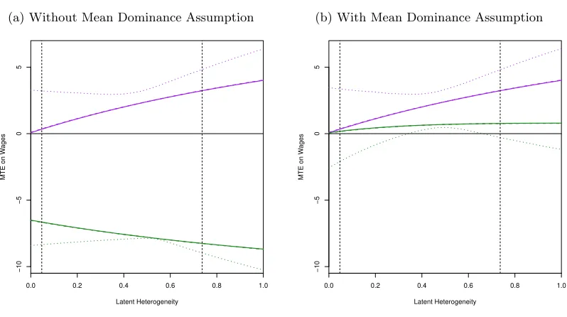
decision (sample selection) by using a partial identification strategy. Although myM T EOO
bounds are uninformative when using only the monotonicity assumption, they are tight and
positive under a mean dominance assumption, illustrating the identification power of extra
assumptions in a context of partial identification. Most interestingly, I find that the bounds
of the M T EOO on hourly wages are decreasing on the likelihood of attending the program,
implying that the agents who benefit the most from the JCTP are the least likely to attend
it. As a consequence of this result, my estimates suggest that ATU is greater than the ATT
for the always-employed subpopulation. Moreover, my bounds on the LAT EOO are in line
with the estimates of Chen & Flores (2015) and the effect of the JCTP on employment is
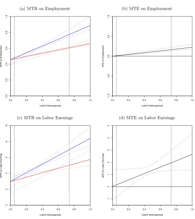
positive for every agent according to the test proposed byMachado et al. (2018). Finally, as
a by product of my estimation strategy, I also find that the MTE on employment and hourly
labor earnings are decreasing on the likelihood of attending the JCTP.
instru-ment, identification of treatment effects with sample selection, and the effect of job training
programs.
The literature about treatment effects with an instrument is enormous and I only briefly
discuss it. Imbens & Angrist(1994) show that we can identify the LATE.Heckman & Vytlacil
(1999), Heckman & Vytlacil (2005) andHeckman et al. (2006) define the MTE and explain
how to compute any treatment effect as a weighted average of the MTE. However, if the
support of the propensity score is not the unit interval, then it is not possible to recover some
important treatment effects, such as the ATE, the ATT and the ATU. A parametric solution
to this problem is given byBrinch et al. (2017), who identify a flexible polynomial function
for the MTE whose degree is defined by the cardinality of the propensity score support.
A nonparametric solution to the impossibility of identifying the ATE and the ATT is
bounding them. Mogstad et al. (2018) use the information contained on IV-like estimands
to construct non-parametrically worst- and best- case bounds on policy-relevant treatment
effects. Other authors focus on imposing weak monotonicity assumptions or a structural
model. In the first group,Manski(1990),Manski(1997) andManski & Pepper(2000) propose
bounds for the ATE and ATT.Chen et al.(2017) propose an average monotonicity condition
combined with a mean dominance condition across subpopulation groups and sharpen the
bounds previously proposed. Huber et al.(2017) add a mean independence condition within
subpopulation groups and bound not only the ATE and ATT when there is noncompliance,
but also the Average Treatment Effect on the Untreated (ATU) and the ATE for always-takers
and never-takers (ATE-AT and ATE-NT).
Complementing the weak monotonicity approach, the structural approach has focused
mainly on the binary outcome case due to the need to impose bounded outcome variables.
Heckman & Vytlacil (2001a), Bhattacharya et al. (2008), Chesher (2010), Chiburis (2010),
Shaikh & Vytlacil (2011) and Bhattacharya et al. (2012) made important contributions to
this literature, bounding the ATE and the ATT. WhileBhattacharya et al.(2008),Shaikh &
Vytlacil(2011) andBhattacharya et al.(2012) consider a thresholding crossing model on the
only on the outcome variable.
I contribute to this literature about identifying treatment effects using an instrument by
extending the non-parametric approach byMogstad et al. (2018) and the flexible parametric
approach byBrinch et al.(2017) to encompass a sample-selection problem. By doing so, I can
partially identify the MTE function on the outcome of interest instead of on the observable
outcome.
The literature about identification of treatment effects with sample selection is vast and
I only briefly discuss it. The control function approach is a possible solution to it and is
analyzed by Heckman (1979), Ahn & Powell (1993) and Newey et al. (1999), encompassing
parametric, semiparametric and nonparametric tools. Using auxiliary data is another
pos-sible solution and is studied by Chen et al. (2008). A nonparametric solution that requires
weaker conditions is bounding. In a seminal paper,Lee (2009) imposes a weak monotonicity
assumption on the relationship between sample selection and treatment assignment to sharply
bound the ITT for the subpopulation of always-observed individuals (IT TOO). Using
tech-niques developed byFrangakis & Rubin (2002),Blundell et al. (2007) andImai (2008) and a
weak monotonicity assumption,Blanco et al. (2013a) bound the Intention-to-Treat Quantile
Treatment Effect for the always-observed individuals (Q−IT TOO). Moreover, by
impos-ing weak dominance assumptions across subpopulation groups, they can sharpen theIT TOO
bounds proposed by Lee (2009). Huber & Mellace (2015) additionally impose a bounded
support for the outcome variable and propose bounds on the ITT for two other
subpopula-tions: observed-only-when-treated individuals (IT TN O), and observed-only-when-untreated
individualsIT TON. Complementary to those studies, Lechner & Mell (2010) derive bounds
for the ITT and the Q-ITT for the treated-and-observed subpopulation, Mealli & Pacini
(2013) derive bounds for the ITT when the exclusion restriction is violated and there are two
outcome variables, and Behaghel et al. (2015) combines techniques developed by Heckman
(1979) and Lee (2009) to propose bounds for the ATE in a survey framework in which the
interviewer tries to contact the surveyed individual multiple times.
selec-tion and endogenous treatment simultaneously. Huber (2014) point-identifies the ATE and
the Quantile Treatment Effect (QTE) for the observed sub-population and for the entire
pop-ulation using a nested propensity score based on an instrument for sample selection. Fricke
et al. (2015) point-identify the LATE by using a random treatment assignment and a
con-tinuous exogenous variable to instrument for treatment status and sample selection. Lee &
Salanie(2016), who also include sample selection in a Generalized Roy Model, use two
con-tinuous instruments to provide control functions for the selection into treatment and sample
selection problems, allowing them to point-identify the MTE.
Although the three previous contributions are important, finding a credible instrument
for sample selection is hard, especially in Labor Economics. For this reason, it is important
to develop tools that do not rely on the existence of an instrument for sample selection.
Frolich & Huber (2014) point-identify the LATE under a predetermined sample-selection
assumption, ruling out an contemporaneous relationship between the potential outcomes and
the sample selection problem. Chen & Flores (2015) derive bounds for Average Treatment
Effect for the always-observed compliers (LATE-OO) by combining one instrument with a
double exclusion restriction with monotonicity assumptions on the sample selection and the
selection into treatment problems. Moreover, Blanco et al. (2017) and Steinmayr (2014)
extend the work by Chen & Flores (2015) by, respectively, considering a censored outcome
variable and analyzing mixture variables combining four strata.
I contribute to the literature about identification of treatment effects with sample selection
by partially identifying the MTE on the always-observed subsample allowing for a
contempo-raneous relationship between the potential outcomes and the sample selection problem, and
using only one (discrete) instrument combined with a monotonicity assumption. Doing so
is theoretically important, because it can unify, in one framework, the bounds for different
treatment effects with sample selection, and empirically relevant, because it allow us to
par-tially identify any treatment effect on the outcome of interest in many empirical problems.
For example, when analyzing the effect of a job training program on wages, it is important
the most from such policy are actually the ones who receive training.
The literature about job training programs is immense and I only briefly discuss it.
Heck-man et al. (1999) wrote an influential survey paper about it, summarizing its main results
and challenges. In particular, after a randomized experiment funded by the U.S. Department
of Labor in 1995, many papers were written about the effects of the Job Corps Training
Pro-gram, such asSchochet et al.(2001) andSchochet et al. (2008). They find that the ITT and
the LATE are positive for educational attainment (GED and vocational certificates),
nega-tive for criminal activity and, posinega-tive for employment and earnings beginning in the third
year after random assignment. With respect to the heterogeneity of treatment effects, their
most interesting result states that there were no employment or earnings effects for Hispanic
youths, a result that is further investigated byFlores-Lagunes et al. (2010). Complementing
those estimates, Chen et al. (2017) partially identifies the ATE and the ATT on earnings,
employment and welfare benefits, finding that they are positive for the first two variables and
negative for the last one. When analyzing heterogeneous treatment effects, their lower bounds
suggest that the treatment is more effective for a treated youth than for a randomly chosen
youth, while their upper bounds support the opposite conclusion.
Finally, the papers that are closer to mine were written by Lee (2009), Blanco et al.
(2013a) andChen & Flores(2015), who analyze the effect of the Job Corps Training Program
on wages by focusing, respectively, on the ITT, the Q-ITT and the LATE parameters for
the always-observed sub-population. Lee (2009) rules out a zero effect after accounting for
the loss in labor market experience generated by the extra education acquired by Job Corps
participants. Blanco et al. (2013a) complement this analysis by finding that the statistically
significantQ−IT TOOfor non-Hispanic youths is between 2.7% and 14% and relatively stable
across different quantiles, while the Q−IT TOO bounds for Hispanic youths are very wide
and include the zero. Chen & Flores (2015) find that the LAT EOO on hourly wages four
years after randomization is between 5.7% and 13.9% for the entire population and between
7.7% and 17.5% for the non-Hispanic population under monotonicity and mean dominance
Program.
I contribute to literature about the Job Corps Training Program by analyzing the MTE for
the Non-Hispanic group, allowing me to understand heterogeneous treatment effects over the
likelihood of attending the program. To summarize those results, I also compute estimates of
theAT EOO, theLAT EOO, theAT TOO and the AT UOO. Moreover, I formally test whether
this training program has a monotone effect on employment by implementing the test proposed
byMachado et al.(2018) for the the non-Hispanic and Hispanic sub-populations. My empirical
results suggests that the agents who are more likely to benefit from the JCTP are the least
likely to attend the program.
This paper proceeds as follows: section 2details the Generalized Roy Model with sample
selection; section3explains how to derive bounds for theM T EOO of interest; sections 4and
5 discuss identification of the M T EOO bounds when the support of the propensity score is
continuous or discrete; and section6 analyzes the effect of the Job Corps Training Program
on hourly wages. Finally, section7 concludes.
2 Framework
I begin with the classical potential outcome framework byRubin(1974) and modify it to
include a sample selection problem. LetZ be an instrumental variable whose support is given
by Z, X be a vector of covariates whose support is given by X, W := (X, Z) be a vector
that combines the covariates and the instrument whose support is given by W :=X × Z,D
be a treatment status indicator, Y∗
0 be the potential outcome of interest when the person is
not treated, and Y∗
1 be the potential outcome of interest when the person is treated. The
outcome variable of interest (e.g., wages) isY∗ :=D·Y1∗+ (1−D)·Y0∗. Moreover, letS1 and
S0 be potential sample selection indicators when treated and when not treated, and define
S:=D·S1+ (1−D)·S0 as the sample selection indicator (e.g., employment status). Define
Y := S ·Y∗ as the observable outcome (e.g., labor earnings). I also define Y1 := S1 ·Y1∗
and Y0 := S0·Y0∗ as the potential observable outcomes. Observe that, following Lee (2009)
direct impact on the potential outcome of interest nor on the sample selection indicator. The
second exclusion restriction requires attention in empirical applications. On the one hand, it
may be a strong assumption in randomized control trials if sample selection is due to attrition
and initial assignment has an effect on the subject’s willingness to contact the researchers.
On the other hand, it may be a reasonable assumption in many labor market applications,
such as the evaluation of a job training program. For example, in my empirical section, it is
reasonable that the initial random assignment to the Job Corps Training Program (JCTP)
has no impact on future employment status.
I model sample selection and selection into treatment using the Generalized Roy Model
(Heckman & Vytlacil 1999). Let U and V be random variables, and P : W → R and
Q:{0,1} × X →Rbe unknown functions. I assume that:
D:=1{P(W)≥U} (1)
and
S :=1{Q(D, X)≥V}. (2)
As Vytlacil (2002) shows, equations (1) and (2) are equivalent to assuming monotonicity
conditions on the selection into treatment problem (Imbens & Angrist (1994)) and on the
sample selection problem (Lee (2009)). I stress that both monotonicity assumptions are
testable using the tools developed byMachado et al. (2018). Note also that, given equation
(2),S0=1{Q(0, X)≥V} and S1 =1{Q(1, X)≥V}.
The random variablesU andV are jointly continuously distributed conditional onX with
densityfU,V|X :R2× X →Rand cumulative distribution functionFU,V|X :R2× X →R. As
is well known in the literature, equations (1) and (2) can be rewritten as
D=1
FU|X (P(W)|X)≥FU|X (U|X) =1
n
˜
P(W)≥U˜o
S=1
FV|X (Q(D, X)|X)≥FV|X (V |X) =1
n
˜
where ˜P(W) :=FU|X (P(W)|X), ˜U :=FU|X (U|X), ˜Q(D, X) :=FV|X (Q(D, X)|X), and
˜
V := FV|X (V |X). Consequently, the marginal distributions of ˜U and ˜V conditional on X
follow the standard uniform distribution. Since this is merely a normalization, I drop the tilde
and mantain throughout the paper the normalization that the marginal distributions of U
andV conditional onX follow the standard uniform distribution and that (P(w), Q(d, x))∈
[0,1]2 for any (x, z, d)∈ W × {0,1}. I also assume that:
Assumption 1 The instrument Z is independent of all latent variables given the covariates
X, i.e., Z ⊥⊥(U, V, Y∗
0, Y1∗)|X.
Assumption 2 The distribution of P(W) givenX is nondegenerate.
Assumption 3 The first and second population moments of the counterfactual variables are
finite, i.e.,E[|Y∗
d|]<+∞, E
h
(Yd∗)2i<+∞, and E[|Sd|]<+∞ for anyd∈ {0,1}.
Assumption 4 Both treatment groups exist for any value of X, i.e., 0<P[D= 1|X]<1.
Assumption 5 The covariates X are invariant to counterfactual manipulations, i.e., X0 =
X1 =X, where X0 and X1 are the counterfactual values of X that would be observed when
the person is, respectively, not treated or treated.
Assumption 6 The potential outcomes Y0∗ and Y1∗ have the same support, i.e., Y∗ :=Y0∗ =
Y1∗, where Y0∗ ⊆R is the support of Y∗
0 and Y1∗ ⊆R is the support ofY1∗.
Assumption 7 Define y∗ := inf{y∈ Y∗} ∈R∪ {−∞} and y∗ := sup{y∈ Y∗} ∈R∪ {∞}.
I assume thaty∗ and y∗ are known, and that
1. y∗ >−∞, y∗=∞ andY∗ is an interval, or
2. y∗ =−∞, y∗<∞ andY∗ is an interval, or
3. y∗ >−∞, y∗<∞ and
(b) y∗ ∈ Y∗ and y∗∈ Y∗.
I stress that assumption 7 is fairly general. Case 1 covers continuous random variables
whose support is convex and bounded below (e.g.: wages), while Case 3.a covers continuous
variables with bounded convex support (e.g.: test scores). Case 3.b encompasses not only
binary variables, but also any discrete variable whose support is finite (e.g.: years of
educa-tion). It also includes mixed random variables whose support is not an interval but achieves
its maximum and minimum. I also highlight that proposition13 shows that assumption 7is
partially necessary to the existence of bounds on theM T EOO of interest in the sense that, if
y∗ =−∞ and y∗ = +∞, then it is impossible to bound the marginal treatment effect on the
outcome of interest for the always-observed sub-population without any extra assumption.
Assumption 8 Treatment has a positive effect on the sample selection indicator for all
in-dividuals, i.e.,Q(1, x)> Q(0, x)>0 for any x∈ X.
Assumption8goes beyond the monotonicity condition implicitly imposed by equation (2)
by assuming that the direction of the effect of treatment on the sample selection indicator
is known and positive, i.e., Q(1, x)≥ Q(0, x) for any x ∈ X. In this sense, it is a standard
assumption in the literature.1 Most importantly, it is also a testable assumption using the tools
developed byMachado et al.(2018), because, under monotone sample selection (equation (2)),
identification of the sign of the ATE on the selection indicator provides a test for Assumption
8. However, Assumption8is slightly stronger than what is usually imposed in the literature,
because it additionally imposes Q(0, x) >0 and Q(1, x) > Q(0, x) for any x ∈ X. I stress
that the first inequality implies that there is a sub-population who is always observed, allowing
me to properly define my target parameter — the marginal treatment effect on the outcome
of interest for the always-observed population (M T EOO). I also highlight that the second
inequality implies that there is a sub-population who is observed only when treated, making
the problem theoretically interesting by eliminating trivial cases of point-identification of the
M T EOOof interest as discussed in proposition10. Finally, I emphasize that all my results can
1
Lee(2009) andChen & Flores(2015) write it in an equivalent way asS1≥S0, whileManski(1997) and
be stated and derived with some obvious changes if I imposeQ(0, x) > Q(1, x)>0 for any
x∈ X instead of Assumption8, as it is done in AppendixC. I also discuss, in AppendixD, an
agnostic approach to monotonicity in the sample selection problem (equation (2)) and show,
in Appendix E, that bounds derived with non-monotone sample selection are uninformative
(i.e., equal to y∗−y∗, y∗−y∗
) under mild regularity conditions.
In my empirical application, Assumption8imposes that the JCTP has a positive effect on
employment for all individuals, which is plausible given the objectives and services provided
by this training program. As discussed by Chen & Flores (2015), the two potential threats
against it — the “lock-in” effect (van Ours(2004)) and an increase in the reservation wage of
treated individuals — are likely to become less relevant in the long-run, justifying my focus
on the hourly wage after 208 weeks from randomization. Most importantly, this assumption
is formally tested by the method developed by Machado et al. (2018) and I reject, at the
1%-significance level, the null hypothesis that Assumption 8 is invalid for the Non-Hispanic
group.
Finally, in partial identification contexts, extra assumptions may have a lot of identification
power. In the specific case of identifying treatment effects with sample selection, it is common
to use mean or stochastic dominance assumptions to tighten the bounds on the parameter of
interest (Imai(2008),Blanco et al.(2013a),Huber & Mellace(2015) andHuber et al.(2017))
and justify them based on the intuitive argument that some population sub-groups have more
favorable underlying characteristics than others. In particular, I discuss the identifying power
of the following mean dominance assumption2:
Assumption 9 The potential outcome when treated for the always-observed sub-population is
greater than or equal to the same parameter for the observed-only-when-treated sub-population:
E[Y1∗|X=x, U =u, S0 = 1, S1= 1 ]≥E[Y1∗|X=x, U =u, S0 = 0, S1= 1 ]
for anyx∈ X and u∈[0,1].
2In appendix F, I derive bounds on the MTE of interest when the above inequality holds in the other
Unfortunately, such assumption is empirically untestable, implying that its use must be
jus-tified for each application based on qualitative or theoretical arguments. In particular, in
my empirical application, it imposes that the marginal treatment response function of wages
when treated for the always-employed population is greater than the same object for the
employed-only-when-treated population. Similarly to the case discussed by Chen & Flores
(2015, section 2.3), Assumption (9) implies a positive correlation between employment and
wages, which is supported by standard models of labor supply.
3 Bounds on the MTEOO
on the outcome of interest
The target parameter, the MTE on the outcome of interest for the sub-population who is
always observed (M T EOO), is given by
∆OOY∗ (x, u) :=E[Y1∗−Y0∗|X=x, U =u, S0= 1, S1 = 1 ]
=E[Y∗
1 |X =x, U =u, S0 = 1, S1 = 1 ]−E[Y0∗|X=x, U =u, S0 = 1, S1= 1 ]
(3)
for any u ∈ [0,1] and any x ∈ X, and is a natural parameter of interest. In labor market
applications where sample selection is due to observing wages only when agents are employed,
it is the effect on wages for the subpopulation who is always employed. In medical applications
where sample selection is due to the death of a patient, it is the effect on health quality for
the subpopulation who survives regardless of the treatment status. In the education literature
where sample selection is due to students quiting school, it is the effect on test scores for the
subpopulation who do not drop out of school regardless of the treatment status. In all those
cases, the target parameter captures the intensive margin of the treatment effect.3
Other possibly interesting parameters are the MTE on the outcome of interest for the
sub-population who is never observed (E[Y∗
1 −Y0∗|X =x, U =u, S0 = 0, S1= 0 ], M T EN N),
3If the researcher is interested in the extensive margin of the treatment effect, captured by the
MTE on the observable outcome (E[Y1−Y0|X=x, U=u]) and by the MTE on the selection indicator
(E[S1−S0|X =x, U =u]), he or she can apply the identification strategies described by Heckman et al.
the MTR function under no treatment for the outcome of interest for the sub-population
who is observed only when treated (E[Y0∗|X=x, U =u, S0= 0, S1 = 1 ],M T R0N O) and MTR
function under treatment for the outcome of interest for the sub-population who is observed
only when treated (E[Y∗
1 |X=x, U =u, S0= 0, S1 = 1 ],M T R1N O). While the last parameter
can be partially identified (Appendix B), the first two parameters are impossible to
point-identify or bound in a informative way because the outcome of interest (Y0∗ or Y1∗) is never
observed for the conditioning sub-populations. Note also that the sub-population who is
observed only when not treated (S0 = 1 and S1 = 0) do not exist by Assumption 8. I
also stress that the conditioning subpopulations in all the above-mentioned parameters are
determined by post-treatment outcomes and, as a consequence, are connected to the statistical
literature known as principal stratification (Frangakis & Rubin(2002)).
I, now, focus on the target parameter ∆OO
Y∗ (x, u) given by equation (3). While
subsec-tion3.1 derives bounds on theM T EOO of interest (equation (3)) using only a monotonicity
assumption (assumptions1-8), subsection 3.2tighten those bounds by additionally imposing
the Mean Dominance Assumption9. Finally, subsection 3.3discusses the empirical relevance
of such bounds.
3.1 Partial Identification with only a Monotonicity Assumption
Here, my goal is to derive bounds on ∆OO
Y∗ (x, u) under assumptions 1-8. Note that the
second right-hand term in equation (3) can be written as4
E[Y0∗|X =x, U =u, S0 = 1, S1 = 1 ] =
mY
0 (x, u)
mS
0 (x, u)
, (4)
where I define mY
0 (x, u) := E[Y0|X =x, U =u] and mS0(x, u) := E[S0|X=x, U =u] as
the MTR functions associated to the counterfactual variablesY0 andS0 respectively. In this
section, I assume that all terms in the right-hand side of equation (4) are point-identified,
postponing the discussion about their identification to sections4and 5.
The first right-hand term in equation (3) can be written as5
E[Y1∗|X=x, U =u, S0 = 1, S1= 1 ] = m
Y
1 (x, u)−∆N OY (x, u)·∆S(x, u)
mS
0 (x, u)
, (5)
where mY1 (x, u) := E[Y1|X =x, U =p] is the MTR function associated to the
counterfac-tual variable Y1, ∆N OY (x, u) := E[Y1−Y0|X =x, U =u, S0 = 0, S1 = 1 ] is the MTE on the
observable outcomeY for the sub-population who is observed only when treated, ∆S(x, u) :=
E[S1−S0|X =x, U =u] = mS
1 (x, u)−mS0(x, u) is the MTE on the selection indicator,
and mS
1 (x, u) :=E[S1|X=x, U =u] is the MTR function associated to the counterfactual
variable S1. In this section, I also assume thatmY1 (x, u) and ∆S(x, u) are point-identified,
postponing the discussion about their identification to sections4and 5.
Although point-identification ofE[Y1∗|X=x, U =u, S0 = 1, S1= 1 ] is not possible, I can
find identifiable bounds for it.6
Proposition 10 Suppose thatmY
0 (x, u),mY1 (x, u),mS0 (x, u)and∆S(x, u)are point-identified.
Under Assumptions 1-6, 7.1 and 8, E[Y∗
1 |X =x, U =u, S0 = 1, S1= 1 ] must satisfy
y∗ ≤E[Y∗
1 |X=x, U =u, S0= 1, S1 = 1 ]≤
mY1 (x, u)−y∗·∆S(x, u)
mS
0 (x, u)
. (6)
Under Assumptions 1-6, 7.2 and 8, E[Y∗
1 |X =x, U =u, S0 = 1, S1= 1 ] must satisfy
mY
1 (x, u)−y∗·∆S(x, u)
mS
0 (x, u)
≤E[Y∗
1 |X =x, U =u, S0 = 1, S1= 1 ]≤y∗. (7)
Under Assumptions1-6,7.3 (sub-case (a) or (b)) and8,E[Y∗
1 |X =x, U =u, S0 = 1, S1 = 1 ]
must satisfy
mY
1 (x, u)−y∗·∆S(x, u)
mS
0 (x, u)
≤E[Y∗
1 |X=x, U =u, S0 = 1, S1= 1 ]
≤ m
Y
1 (x, u)−y∗·∆S(x, u)
mS
0 (x, u)
. (8)
5
AppendixA.2contains a proof of this claim.
6
There is a important remark to be made about the bounds of proposition 10. Note that,
even when the support is bounded in only one direction (assumptions 7.1 and 7.2), it is
possible to derive lower and upper bounds onE[Y∗
1 |X=x, U =u, S0= 1, S1 = 1 ].
At this point, it is also important to understand the determinants of the width of those
bounds. First, if there is no sample selection problem at all (P[S0 = 1, S1 = 1|X=x, U =u] =
1), then mS
0 (x, u) = 1, ∆S(x, u) = 0, implying tighter bounds in equations (6) and (7) and
point-identification in equation (8). Second and most importantly, if there is no problem of
dif-ferential sample selection with respect to treatment status (P[S0= 0, S1 = 1|X =x, U =u] =
0), then ∆S(x, u) = 0, once more implying tighter bounds in equations (6) and (7) and
point-identification in equation (8). Both cases are theoretically uninteresting and ruled out by
Assumption8.
Finally, combining equations (3) and (4) and proposition 10, I can partially identify the
target parameter ∆OO Y∗ (x, u):
Corollary 11 Suppose thatmY0 (x, u),mY1 (x, u),mS0 (x, u)and∆S(x, u)are point-identified.
Under Assumptions 1-6, 7.1 and 8, the bounds on∆OO
Y∗ (x, u) are given by
∆OOY∗ (x, u)≥y∗−
mY
0 (x, u)
mS
0 (x, u)
=: ∆OOY∗ (x, u) (9)
and that
∆OOY∗ (x, u)≤
mY
1 (x, u)−y∗·∆S(x, u)
mS
0 (x, u)
−m
Y
0 (x, u)
mS
0(x, u)
=: ∆OO
Y∗ (x, u). (10)
Under Assumptions 1-6, 7.2 and 8, the bounds on∆OO
Y∗ (x, u) are given by
∆OOY∗ (x, u)≥
mY
1 (x, u)−y∗·∆S(x, u)
mS
0 (x, u)
−m
Y
0 (x, u)
mS
0 (x, u)
=: ∆OOY∗ (x, u) (11)
and that
∆OOY∗ (x, u)≤y∗−
mY
0 (x, u)
mS
0 (x, u)
=: ∆OO
Y∗ (x, u). (12)
given by
∆OOY∗ (x, u)≥max
mY
1 (x, u)−y∗·∆S(x, u)
mS
0(x, u)
, y∗
−m
Y
0 (x, u)
mS
0 (x, u)
=: ∆OOY∗ (x, u) (13)
and that
∆OOY∗ (x, u)≤min
(
mY
1 (x, u)−y∗·∆S(x, u)
mS
0 (x, u)
, y∗
)
−m
Y
0 (x, u)
mS
0 (x, u)
=: ∆OO
Y∗ (x, u). (14)
Most importantly, I can show that7:
Proposition 12 Suppose that the functions mY
0, mY1, mS0 and ∆S are point-identified at
every pair(x, u)∈ X ×[0,1]. Under Assumptions1-6,7 (sub-cases 1, 2, 3(a) or 3(b)) and8,
the bounds∆OO
Y∗ and ∆OOY∗, given by corollary11, are point-wise sharp, i.e., for anyu∈[0,1],
x∈ X and δ(x, u) ∈∆OO
Y∗ (x, u),∆OOY∗ (x, u)
, there exist random variables Y˜0∗,Y˜1∗,U ,˜ V˜
such that
∆OOY˜∗ (x, u) :=E
h
˜
Y1∗−Y˜0∗
X =x,U˜ =u,S˜0 = 1,S˜1= 1 i
=δ(x, u), (15)
P
h
˜
Y0∗,Y˜1∗,V˜∈ Y∗× Y∗×[0,1]
X=x,
˜
U =ui= 1 for anyu∈[0,1], (16)
and
FY ,˜ D,˜S,Z,X˜ (y, d, s, z, x) =FY,D,S,Z,X(y, d, s, z, x) (17)
for any (y, d, s, z) ∈ R4, where D˜ := 1
n
P(X, Z)≥U˜o, S˜0 = 1
n
Q(0, X)≥V˜o, S˜1 =
1nQ(1, X)≥V˜o, Y˜0= ˜S0·Y˜0∗, Y˜1 = ˜S1·Y˜1∗ and Y˜ = ˜D·Y˜1+
1−D˜·Y˜0.
Intuitively, proposition 12 says that, for any δ(x, u) ∈ ∆OO
Y∗ (x, u),∆OOY∗ (x, u)
, it is
possible to create candidate random variables Y˜∗
0,Y˜1∗,U ,˜ V˜
that generate the candidate
marginal treatment effect δ(x, u) (equation (15)), satisfy the bounded support condition —
a restriction imposed by my model (Assumption7) and summarized in equation (16) — and
7
AppendixA.4contains the proof of this proposition. Note that, if the functionsmY0,mY1,mS0 and ∆Sare
generate the same distribution of the observable variables — a restriction imposed by the
data and summarized in equation (17). In other words, the data and the model in section
2 do not generate enough restrictions to refute that the true target parameter ∆OO
Y∗ (x, u) is
equal to the candidate target parameterδ(x, u).
Moreover, the bounded support condition (Assumption 7) is partially necessary to the
existence of bounds on the target parameter ∆OO
Y∗ (x, u). When the support is unbounded in
both directions (i.e.,y∗ =−∞ and y∗ = +∞), then it is impossible to derive bounds on the
target parameter ∆OO
Y∗ (x, u) without any extra assumption. Proposition 13 formalizes this
last statement.8
Proposition 13 Suppose that the functions mY
0, mY1, mS0 and ∆S are point-identified at
every pair (x, u) ∈ X × [0,1]. Impose assumptions 1-6 and 8. If Y∗ = R, then, for any
u∈[0,1], x∈ X and δ(x, u)∈R, there exist random variables
˜
Y0∗,Y˜1∗,U ,˜ V˜ such that
∆OOY˜∗ (x, u) :=E
h
˜
Y1∗−Y˜0∗
X =x,
˜
U =u,S˜0 = 1,S˜1= 1
i
=δ(x, u), (18)
P
h
˜
Y0∗,Y˜1∗,V˜∈ Y∗× Y∗×[0,1]
X=x,U˜ =u i
= 1 for anyu∈[0,1], (19)
and
FY ,˜ D,˜S,Z,X˜ (y, d, s, z, x) =FY,D,S,Z,X(y, d, s, z, x) (20)
for any (y, d, s, z) ∈ R4, where D˜ := 1
n
P(X, Z)≥U˜o, S˜0 = 1
n
Q(0, X)≥V˜o, S˜1 =
1nQ(1, X)≥V˜o, Y˜0= ˜S0·Y˜0∗, Y˜1 = ˜S1·Y˜1∗ and Y˜ = ˜D·Y˜1+
1−D˜·Y˜0.
In other words, when the support of the potential outcome is the entire real line, the data
and the model in section2 do not generate enough restrictions to refute that the true target
parameter ∆OO
Y∗ (x, u) is equal to an arbitrarily large effect in magnitude. This impossibility
result is interesting in light of the previous literature about partial identification of treatment
effects with sample selection. In the case of theIT TOO (Lee(2009)) and theLAT EOO (Chen
& Flores(2015)), it is possible to construct informative bounds even when the support of the
potential outcome is the entire real line. However, when focusing on a specific point of the
M T EOO function, it is impossible to construct informative bounds when Y∗ =R due to the
local nature of the target parameter.
There is one important remark about the results I have just derived. Note that
propo-sitions 12 and 13 do not impose any smoothness condition on the joint distribution of
(Y0∗, Y1∗, U, V, Z, X). In particular, the conditional cumulative distribution functionsFV|X,U,
FY∗
0|X,U,V and FY
∗
1|X,U,V are allowed to be discontinuous functions of U at the point u.
Ap-pendixG states and proves a sharpness result similar to proposition12 and an impossibility
result similar to proposition13 when FV|X,U, FY∗
0|X,U,V and FY
∗
1|X,U,V must be continuous
functions of U.
3.2 Partial Identification with an Extra Mean Dominance Assumption
Here, I use the Mean Dominance Assumption 9 to tighten the bounds on the target
parameter ∆OOY∗ (equation (3)) given by corollary 11. Note that Assumption 9 implies that
∆N OY (x, u)≤ m
Y
1 (x, u)
mS
1(x, u)
≤E[Y1∗|X =x, U =u, S0 = 1, S1= 1 ] by equations (A.4) and (A.5).
As a consequence, by following the same steps of the proof of corollary11, I can derive:
Corollary 14 Fix u ∈ [0,1] and x ∈ X arbitrarily. Suppose that the mY
0 (x, u), mY1 (x, u),
mS0 (x, u) and ∆S(x, u) are point-identified.
Under Assumptions 1-6, 7.1, 8 and 9, ∆OOY∗ (x, u) must satisfy
∆OOY∗ (x, u)≥
mY
1 (x, u)
mS
1 (x, u)
−m
Y
0 (x, u)
mS
0 (x, u)
=: ∆OOY∗ (x, u) (21)
and that
∆OOY∗ (x, u)≤
mY
1 (x, u)−y∗·∆S(x, u)
mS
0 (x, u)
−m
Y
0 (x, u)
mS
0(x, u)
=: ∆OO
Y∗ (x, u). (22)
Under Assumptions 1-6, 7.2, 8 and 9, ∆OO
Y∗ (x, u) must satisfy
∆OOY∗ (x, u)≥
mY
1 (x, u)
mS
1 (x, u)
−m
Y
0 (x, u)
mS
0 (x, u)
and that
∆OOY∗ (x, u)≤y∗−
mY
0 (x, u)
mS
0 (x, u)
=: ∆OO
Y∗ (x, u). (24)
Under Assumptions 1-6, 7.3 (sub-case (a) or (b)), 8 and 9, ∆OO
Y∗ (x, u) must satisfy
∆OOY∗ (x, u)≥
mY1 (x, u)
mS
1 (x, u)
−m
Y
0 (x, u)
mS
0 (x, u)
=: ∆OOY∗ (x, u) (25)
and that
∆OOY∗ (x, u)≤min
(
mY
1 (x, u)−y∗·∆S(x, u)
mS
0 (x, u)
, y∗
)
−m
Y
0 (x, u)
mS
0 (x, u)
=: ∆OO
Y∗ (x, u). (26)
When Y∗=R and Assumptions 1-6, 8 and 9 hold, ∆OO
Y∗ (x, u) must satisfy
∆OOY∗ (x, u)≥
mY1 (x, u)
mS
1 (x, u)
−m
Y
0 (x, u)
mS
0 (x, u)
=: ∆OOY∗ (x, u) (27)
and that
∆OOY∗ (x, u)≤ ∞=: ∆OOY∗ (x, u). (28)
Notice that, under Mean Dominance Assumption 9, I can increase the lower bounds
pro-posed in corollary11under Assumption7and provide an informative lower bound even when
the support of the outcome of interest is the entire real line, a result in stark contrast with
proposition13. These improvements clearly show the identifying power of the Mean
Domi-nance Assumption9.
As in subsection3.1, I assume thatmY
0 (x, u),mY1 (x, u),mS0 (x, u),mS1 (x, u), and ∆S(x, u)
are point-identified, postponing the discussion about their identification to sections4and 5.
Now, using the above corollary, I can combine the sharpness and the impossibility results
of subsection3.1 in one single proposition9:
Proposition 15 Suppose that the functions mY
0, mY1, m0S, mS1 and ∆S are point-identified
at every pair(x, u)∈ X ×[0,1]. Under Assumptions1-6,8 and9, the bounds∆OO
Y∗ and∆OOY∗,
9
given by corollary 14, are point-wise sharp, i.e., for any u ∈ [0,1], x ∈ X and δ(x, u) ∈
∆OOY∗ (x, u),∆OOY∗ (x, u)
, there exist random variables Y˜0∗,Y˜1∗,U ,˜ V˜ such that
∆OOY˜∗ (x, u) :=E
h
˜
Y1∗−Y˜0∗
X =x,U˜ =u,S˜0 = 1,S˜1= 1 i
=δ(x, u), (29)
P
h
˜
Y0∗,Y˜1∗,V˜∈ Y∗× Y∗×[0,1]
X=x,
˜
U =ui= 1 for anyu∈[0,1], (30)
E
h
˜
Y1∗
X =x,U˜ =u,S˜0 = 1,S˜1 = 1 i
≥E
h
˜
Y1∗
X=x,U˜ =u,S˜0 = 0,S˜1= 1 i
, (31)
and
FY ,˜ D,˜S,Z,X˜ (y, d, s, z, x) =FY,D,S,Z,X(y, d, s, z, x) (32)
for any (y, d, s, z) ∈ R4, where D˜ := 1
n
P(X, Z)≥U˜o, S˜0 = 1
n
Q(0, X)≥V˜o, S˜1 =
1nQ(1, X)≥V˜o, Y˜0= ˜S0·Y˜0∗, Y˜1 = ˜S1·Y˜1∗ and Y˜ = ˜D·Y˜1+
1−D˜·Y˜0.
Note that, in addition to all the restriction imposed by proposition 12, the candidate
random variablesY˜∗
0,Y˜1∗,U ,˜ V˜
must also satisfy an extra model restriction (equation (31))
associated to the Mean Dominance Assumption 9.
3.3 Empirical Relevance of Bounds on the MTEOO of Interest
Now, it is important to discuss the empirical relevance of partially identifying theM T EOO
of interest. First, bounds on theM T EOO can illuminate the heterogeneity of the treatment
effect, allowing the researcher to understand who benefits and who loses with a specific
treat-ment. This is important because common parameters (e.g.: AT EOO, AT TOO, AT UOO,
LAT EOO) can be positive even when most people lose with a policy if the few winners have
very large gains. Moreover, knowing, even partially, the M T EOO function can be useful to
optimally design policies that provides incentives to agents to take some treatment. Second,
I can use the M T EOO bounds to partially identify any treatment effect that is described as
a weighted integral of ∆OO
Y∗ (x, u) because
Z 1
0
∆OOY∗ (x, u)
·ω(x, u) du≤
Z 1
0
≤
Z 1
0
∆OO Y∗ (x, u)
·ω(x, u) du, (33)
where ω(x,·) is a known or identifiable weighting function. Even though such bounds may
not be sharp for any specific parameter, they are a general and off-the-shelf solution to many
empirical problems. As a consequence of this trade-off, I recommend the applied researcher to
use a specialized tool if he or she is interested in a parameter that already has specific bounds
for it (e.g., ITT byLee(2009) and LATE byChen & Flores(2015)). However, I suggest the
applied research to easily compute a weighted integral of point-wise sharp bounds on the MTE
of interest if he or she is interested in parameters without specialized bounds (e.g., ATE, ATT
and ATU in the case with imperfect compliance). In other words, facing a trade-off between
empirical flexibility and sharpness, the partial identification tool proposed in this paper focus
on empirical flexibility while still ensuring point-wise sharpness of the bounds on the MTE of
interest.
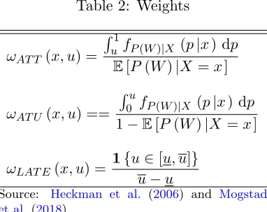
Tables1and2show some of the treatment effect parameters that can be partially identified
using inequality (33). More examples are given by Heckman et al.(2006, Tables 1A and 1B)
andMogstad et al. (2018, Table 1).
Table 1: Treatment Effects as Weighted Integrals of the Marginal Treatment Effect
AT EOO=E[Y∗
1 −Y0∗|S0= 1, S1 = 1 ] =
R1
0 ∆OOY∗ (u) du
AT TOO=E[Y1∗−Y0∗|D= 1, S0= 1, S1 = 1 ] =R1 0 ∆
OO
Y∗ (u)·ωAT T (u) du
AT UOO=E[Y∗
1 −Y0∗|D= 0, S0 = 1, S1 = 1 ] =
R1
0 ∆OOY∗ (u)·ωAT U(u) du
LAT EOO(u, u) =E[Y∗
1 −Y0∗|U ∈[u, u], S0= 1, S1 = 1 ] =
R1
Table 2: Weights
ωAT T(x, u) =
R1
u fP(W)|X (p|x) dp
E[P(W)|X =x]
ωAT U(x, u) ==
Ru
0 fP(W)|X (p|x) dp
1−E[P(W)|X =x]
ωLAT E(x, u) =
1{u∈[u, u]}
u−u
Source: Heckman et al. (2006) and Mogstad et al.(2018).
4 Partial identification when the support of the propensity score is an
interval
Here, I fix x ∈ X and impose that the support of the propensity score, defined by
Px := {P(x, z) :z∈ Z}, is an interval10. Then, under assumptions 1-5, the MTR functions
associated to any variableA∈ {Y, S} are point-identified by11:
mA0 (x, p) =E[A|X=x, P (W) =p, D= 0 ]−∂E[A|X=x, P (W) =p, D= 0 ]
∂p ·(1−p),
(34)
and
mA1 (x, p) =E[A|X =x, P(W) =p, D= 1 ] + ∂E[A|X =x, P(W) =p, D= 1 ]
∂p ·p (35)
for any p∈ Px.
Finally, the point-wise sharp bounds on ∆OO
Y∗ (x, p) are point-identified by combining
equa-tions (34) and (35), the fact that ∆S(x, p) =mS1 (x, p)−mS0 (x, p), and Corollaries11 or14.
10P
x as an interval may be achieved by a continuous instrument Z or by the existence of independent
covariates (Carneiro et al. 2011).
11
5 Partial identification when the support of the propensity score is discrete
When the support of the propensity score is not an interval, I cannot point-identify
mY
0 (x, u),mY1 (x, u),mS0 (x, u),mS1 (x, u), and ∆S(x, u) without extra assumptions, implying
that I cannot identify the bounds on ∆OO
Y∗ (x, u) given by Corollaries11 or14. There are two
solutions for such lack of identification: I can non-parametrically bound those four objects
(Mogstad et al.(2018)) or I can impose flexible parametric assumptions (Brinch et al.(2017))
to point-identify them. While the first approach is discussed in subsection5.1, the second one
is detailed in subsection5.2.
5.1 Non-parametric outer set around the MTEOO of interest
For any u∈[0,1] and x∈ X, I can boundmY0 (x, u), mY1 (x, u), mS0 (x, u), mS1 (x, u), and
∆S(x, u) using the machinery proposed by Mogstad et al.(2018). To do so, fix A ∈ {Y, S}
and d ∈ {0,1} and define the pair of functions mA := mA
0, mA1
and the set of admissible
MTR functions MA ∋ mA. Furthermore, fix (x, u) ∈ X ×[0,1] and define the functions
Γ∗1:MY →R, Γ∗
2:MY →R, Γ∗3:MS →R, Γ∗4:MS→Rand Γ∗5:MS →Ras:
Γ∗1 m˜Y
= ˜mY1 (x, u) + 0·m˜Y0 (x, u)
Γ∗2 m˜Y
= 0·m˜Y1 (x, u) + ˜mY0 (x, u)
Γ∗3 m˜S
= 0·m˜S1 (x, u) + ˜mS0 (x, u)
Γ∗4 m˜S
= ˜mS1 (x, u) + 0·m˜S0 (x, u)
Γ∗5 m˜S
= ˜mS1 (x, u)−m˜S0 (x, u),
and observe that Γ∗1 mY
=mY
1 (x, u), Γ∗2 mY
=mY
0 (x, u), Γ∗3 mS
=mS
0 (x, u), Γ∗4 mS
=
mS
1 (x, u), and Γ∗5 mS
= ∆S(x, u). Moreover, define, for eachA∈ {Y, S},GAto be a
collec-tion of known or identified measurable funccollec-tionsgA: {0,1}×X ×Z →Rwhose second moment
According to proposition 1 byMogstad et al.(2018), the function ΓgA:M
A→R, defined as
ΓgA m˜
A
=E
Z 1
0
˜
mA0 (X, u)·gA(0, Z)·1{p(W)< u} du
X=x
+E
Z 1
0
˜
mA1 (X, u)·gA(1, Z)·1{p(W)≥u} du
X=x
,
satisfies ΓgA m
A
= βgA. As a result, m
A must lie in the set M
GA of admissible functions
that satisfy the restrictions imposed by the data through the IV-like specifications, where:
MGA :=
˜
mA∈ MA: Γ
gA m˜
A
=βgA for all gA∈ GA .
Assuming thatMAis convex andM
GA 6=∅for everyA∈ {Y, S}, proposition 2 byMogstad
et al.(2018) ensures that:
inf
˜
mY∈MG Y
Γ∗
1 m˜Y
=:mY
1 (x, u)≤ mY1 (x, u) ≤mY1 (x, u) := sup ˜
mY∈MG Y
Γ∗
3 m˜Y
inf
˜
mY∈MG Y
Γ∗
2 m˜Y
=:mY
0 (x, u)≤ mY0 (x, u) ≤mY0 (x, u) := sup ˜
mY∈MG Y
Γ∗
2 m˜Y
inf
˜
mS∈MG S
Γ∗3 m˜S
=:mS0 (x, u)≤ mS0 (x, u) ≤mS
0 (x, u) := sup ˜
mS∈MG S
Γ∗3 m˜S
inf
˜
mS∈MG S
Γ∗4 m˜S
=:mS
1 (x, u)≤ mS1 (x, u) ≤mS1 (x, u) := sup ˜
mS∈MG S
Γ∗4 m˜S
inf
˜
mS∈MG S
Γ∗5 m˜S
=: ∆S(x, u)≤ ∆S(x, u) ≤∆S(x, u) := sup
˜
mS∈MG S
Γ∗5 m˜S
(36)
As a consequence, I can combine Corollary 11 and inequalities (36) to provide a
non-parametrically identified outer set around ∆OO Y∗ (x, u):
Corollary 16 Fix u∈[0,1]and x∈ X arbitrarily.
Under assumptions1-6,7.1 and8, the bounds of an outer set around ∆OO
Y∗ (x, u) are given
by
∆OOY∗ (x, u)≥y∗−
mY
0 (x, u)
mS
0 (x, u)
, (37)
and that
∆OOY∗ (x, u)≤
mY
1 (x, u)
mS
0(x, u)
−y
∗·∆ S(x, u)
mS
0 (x, u)
−m
Y
0 (x, u)
mS
0 (x, u)
Under assumptions1-6,7.2 and8, the bounds of an outer set around ∆OOY∗ (x, u) are given
by
∆OOY∗ (x, u)≥
mY
1 (x, u)
mS
0(x, u)
−y
∗·∆ S(x, u)
mS
0 (x, u)
−m
Y
0 (x, u)
mS
0 (x, u)
, (39)
and that
∆OOY∗ (x, u)≤y∗−
mY
0 (x, u)
mS
0 (x, u)
. (40)
Under assumptions1-6,7.3 (sub-case (a) or (b)) and8, the bounds of an outer set around
∆OO
Y∗ (x, u) are given by
∆OOY∗ (x, u)≥max
(
max
(
mY
1 (x, u)
mS
0 (x, u)
−y
∗·∆ S(x, u)
mS
0 (x, u) , y∗
)
− m
Y
0 (x, u)
mS
0 (x, u)
, y∗−y∗
)
, (41)
and that
∆OOY∗ (x, u)≤min
(
min
(
mY
1 (x, u)
mS
0 (x, u)
−y
∗·∆ S(x, u)
mS
0 (x, u) , y∗
)
−m
Y
0 (x, u)
mS
0 (x, u)
, y∗−y∗
)
. (42)
Note that I can obviously combine Corollary14and inequalities (36) to derive the bounds
of an outer set around ∆OO
Y∗ (x, u) under the Mean Dominance Assumption 9. Moreover, I
stress that the cost of non-parametric partial identification ofmY
0 (x, u),mY1 (x, u),mS0 (x, u),
mS
1 (x, u), and ∆S(x, u) is losing the point-wise sharpness of the bounds around the target
parameter ∆OO
Y∗. For that reason, Corollary 16 is stated in terms of bounds of an outer set
around ∆OO
Y∗ (x, u), that contains the true target parameter ∆OOY∗ (x, u) by construction.
5.2 Parametric identification of the MTEOO
bounds
The fully non-parametric approach explained in subsection 5.1 may provide an
uninfor-mative outer set (e.g., equal toy∗−y∗ ory∗−y∗ when the support of the potential outcome is
bounded). In such cases, parametric assumptions on the marginal treatment response function
may buy a lot of identifying power. Although restrictive in principle, parametric assumptions
may be flexible enough to provide credible bounds on ∆OOY∗ (x, u).
given by Px = {px,1, . . . , px,N} for some N ∈ N. I could directly apply the identification
strategy proposed byBrinch et al.(2017) by assuming that the MTR functions associated to
Y and S are polynomial functions of U. However, this assumption is problematic for binary
variables, such as the selection indicatorS. For this reason, I make a small modification to the
procedure created byBrinch et al. (2017): for d∈ {0,1} and A ∈ {Y, S}, the MTR function
is given by
mAd (x, u) =MA u,θAx,d (43)
for any u ∈ [0,1], where ΘAx ⊂ R2L is a set of feasible parameters, L ∈ {1, . . . , N} is the
number of parameters for each treatment group d, θAx,
0,θAx,1
∈ ΘA
x is a vector of
pseudo-true unknown parameters, and MA: [0,1]×R2L → R is a known function. For example,
in the case of a binary variable, a reasonable choice of MA is the Bernstein Polynomial
MA u,θA
x,d
=PL−1
l=0 θx,d,lA · L−1
l
·ul·(1−u)L−1−l
with feasible set ΘA
x = [0,1]2 L
. In the
case of the selection indicator, the feasible set would be further restricted by Assumption
8 to ΘA x =
n
˜
θAx,0,θ˜Ax,1
∈[0,1]2L:θ˜Ax,1 ≥θ˜Ax,0
o
. I stress that the only difference between
the Bernstein polynomial model and the simple polynomial model proposed byBrinch et al.
(2017) is that it is easier to impose feasibility restrictions on the former model.
Back to the parametric model given by equation (43), I define the parameters θAx,
0,θAx,1
as
pseudo-true parameters in the sense that the parametric model in equation (43) is an
approxi-mation to the true data generating process via the momentsE[A|X=x, P (W) =pn, D=d]
for any d∈ {0,1}and n∈ {1, . . . , N}. Formally, I define
θAx,
0,θAx,1
:= argmin
˜
θAx,0,θ˜Ax,1
∈ΘA x N X n=1
E[A|X =x, P(W) =pn, D= 0 ]−
R1
pnM
Au,θ˜A x,0
du
1−pn
2
+
E[A|X=x, P(W) =pn, D= 1 ]− Rpn
0 MA
u,θ˜Ax,
1 du pn 2 . (44)
equation (44), i.e., I only have to estimate a constrained OLS regression whose restrictions are
given by the set ΘAx. If the model restrictions imposed through the set of feasible parameters
ΘA
x are valid and L = N, then my parametric model collapses to the model proposed by
Brinch et al.(2017) and I find that12, for any p
n∈ Px,
E[A|X =x, P(W) =pn, D= 0 ] =
R1
pnM
A u,θA x,0
du
1−pn
(45)
E[A|X =x, P(W) =pn, D= 1 ] =
Rpn
0 MA u,θ
A x,1
du pn
. (46)
I can, then, combine Corollary11 and equations (43) and (44) to bound ∆OOY∗ (x, u):
Corollary 17 Fix u∈[0,1]and x∈ X arbitrarily.
Under assumptions 1-6, 7.1 and 8, the bounds on∆OO
Y∗ (x, u) are given by
∆OOY∗ (x, u)≥y∗−
MY u,θY
x,0
MS u,θS
x,0
, (47)
and that
∆OOY∗ (x, u)≤
MY u,θY
x,1
−y∗·
MS u,θS
x,1
−MS u,θS
x,0
MS u,θS
x,0
−
MY u,θY
x,0
MS u,θS
x,0
. (48)
Under assumptions 1-6, 7.2 and 8, the bounds on∆OO
Y∗ (x, u) are given by
∆OOY∗ (x, u)≥
MY u,θY
x,1
−y∗·
MS u,θS
x,1
−MS u,θS
x,0
MS u,θS
x,0
−
MY u,θY
x,0
MS u,θS
x,0
, (49)
and that
∆OOY∗ (x, u)≤y∗−
MY u,θY
x,0
MS u,θSx,
0
. (50)
Under assumptions 1-6, 7.3 (sub-case (a) or (b)) and 8, the bounds on ∆OO
Y∗ (x, u) are
12
given by
∆OOY∗ (x, u)≥max
(
MY u,θY
x,1
−y∗·
MS u,θS
x,1
−MS u,θS
x,0
MS u,θS
x,0
, y
∗
)
−M
Y u,θY x,0
MS u,θS
x,0
,
(51)
and that
∆OOY∗ (x, u)≤min
(
MY u,θYx,
1
−y∗·
MS u,θSx,
1
−MS u,θSx,
0
MS u,θS
x,0
, y
∗
)
−M
Y u,θY x,0
MS u,θS
x,0
.
(52)
Note that I can obviously combine Corollary 14 and equations (43) and (44) to bound
∆OO
Y∗ (x, u) under the Mean Dominance Assumption9.
6 Empirical Application: Job Corps Training Program
Active Labor Market Programs are a common way to possibly fight unemployment and
increase wages by providing public employment services, labor market training and subsidized
employment. Given their economic importance, they were extensively studied in the literature:
Heckman et al.(1999),Heckman & Smith (1999),Abadie et al. (2002) and van Ours(2004).
In particular, the Job Corps Training Program (JCTP) received great academic attention
(Schochet et al. (2001), Schochet et al. (2008), Flores-Lagunes et al. (2010), Flores et al.
(2012),Blanco et al.(2013a),Blanco et al.(2013b),Chen & Flores(2015),Chen et al.(2017),
Blanco et al. (2017)) due to its randomized evaluation funded by the U.S. Department of
Labor in the mid 1990’s.
For its social and academic importance, I focus on analyzing the Marginal Treatment Effect
of the JCTP on wages for the always-employed sub-population (M T EOO). This program
provides free education and vocational training to individuals who are legal residents of the
U.S., are between the ages of 16 and 24 and come from a low-income household (Schochet
et al.(2001) andLee(2009)). Besides receiving education and vocational training, the trainees
reside in the Job Corps center, that offers meals and a small cash allowance.