Improving the Effectiveness of Weather based Insurance: An Application of Copula Approach

(1)

Munich Personal RePEc Archive

Improving the Effectiveness of

Weather-based Insurance: An

Application of Copula Approach

Bokusheva, Raushan

ETH Zurich (Swiss Federal Institute of Technology)

22 January 2014

Online at

https://mpra.ub.uni-muenchen.de/62339/

(2)

IMPROVING THE EFFECTIVENESS OF WEATHER-BASED INSURANCE:

AN APPLICATION OF COPULA APPROACH

Raushan Bokusheva

Agricultural Economics, ETH Zurich bokushev@ethz.ch

Abstract

The study develops the methodology for a copula-based weather index insurance

rating. As the copula approach is better suited for modeling tail dependence than the

standard linear correlation method, we suppose that copulas are more adequate for

pricing a weather index insurance contract against extreme weather events. To capture

the dependence structure in the left tail of the joint distribution of a weather variable

and the farm yield, we employ the Gumbel survival copula. Our results indicate that,

given the choice of an appropriate weather index to signal extreme drought

occurrence, a copula-based weather insurance contact might provide higher risk

reduction compared to a regression-based indemnification.

Keywords: catastrophic insurance, weather index insurance, copula, insurance

contract design

(3)

INTRODUCTION

Weather index insurance has been considered as a valuable alternative for traditional

crop insurance. The main advantage of the former is that it is better suited to combat

asymmetric information problems, that is, adverse selection and moral hazard. An

additional important advantage of weather-based insurance is that it considerably

reduces transaction costs and thus allows a faster settlement of claims. The latter

characteristic of weather index insurance makes it particularly relevant in the context

of extreme weather event management, when the relief must be provided within a

short period of time to a large number of affected farms.

Yet, as recent empirical evidence shows, despite substantial efforts of developing

agencies such as the World Bank and governmental support to promote the market of

weather index insurance in a number of developing countries, the demand for this

instrument of risk reduction remains rather low (Cole et al. 2013; Mobarak and

Rosenzweig 2012; Norton et al. 2011). Recent empirical studies examine and discuss

different factors affecting farmers’ demand for weather index insurance. In addition

to factors evaluated in the context of traditional agricultural insurance such farm’s

socio-economic characteristics as risk aversion, level of production diversification

etc., the literature discusses the effect of informal insurance (Mobarak and

Rosenzweig 2012; Akter and Fatema 2011), basis risk (Barnett and Mahul 2010), and

model prediction uncertainties (Bokusheva and Breustedt 2012).

Given this recent evidence, we analyze an option which would address the above

mentioned issues and potentially increase risk reducing effectiveness of weather index

insurance. We propose to design weather index insurance as an insurance against

extreme events rather than an instrument to cope with moderate weather risks, as has

been done in previous studies (Wang et al. 2013; Breustedt et al. 2008; Vedenov and

Barnett 2004; Skees et al. 1997). In our view, this approach should positively

influence the demand for weather index insurance as it could: (i) improve

affordability of weather index insurance; (ii) reduce scope of basis risk; and (iii)

improve predictive power of yield-weather models used for insurance contract rating.

(i) The presence of informal insurance might reduce demand for formal insurance

against moderate risks due to a certain capacity of rural communities to share risk

(4)

within a rural community might be insufficient to cope with catastrophic risks, which

usually have a systemic character and thus affect a large number of producers

simultaneously. Accordingly, wealthier households of a community themselves might

experience substantial yield losses in the case of a catastrophic event, which would

affect their capacity and willingness to provide informal insurance to other members

of the community. In this context, weather index insurance designed to cope with

catastrophic risks might be better targeted to the needs of rural households, compared

to insurance products insuring against moderate yield losses: moderate losses would

be covered by using informal insurance, while extreme yield losses would be

indemnified by a catastrophic weather index insurance.

(ii) The main reasons for basis risk are: (a) a low correlation of farm yields with a

weather index due to the presence of other important risks, namely those beyond the

hazard, to be insured by a particular weather-based insurance product (i.e., so-called

loss-specific basis risk); (b) a low sensitivity of the farm yield to weather data of

meteorological stations situated at a considerable distance to the farm (i.e., spatial

basis risk); and (c) a low correlation between a weather index and a crop yield due to

the timing of the occurrence of the insured event (i.e., temporal basis risk) (Skees et

al. 2007). We presume that catastrophic weather index insurance against catastrophic

events might be less affected by spatial basis risk as extreme events have a higher

extent of spatial correlation. Compared to common weather index insurance, it would

indemnify insured farms less frequently, but would potentially allow a more adequate

coverage for yield losses in the case of extreme events.

(iii) Finally, we suppose that the application of methods appropriate for modeling

extreme dependence, such as copulas could provide more robust estimates of yield

dependence on weather and, thus, substantially limit the scope for model prediction

uncertainties.

In our study, we evaluate the effectiveness of a catastrophic weather index insurance

against drought by applying two alternative methods—the standard regression

analysis and the copula approach. Most empirical analyses obtain estimates of the

dependence of crop yields on a weather index by assuming a linear correlation

structure in yield-weather dependence; i.e. they regard yield-weather distribution as a

Gaussian multivariate distribution. This procedure has an important implication: the

(5)

over the whole distribution of the conditioning variable—the weather index. We

argue that, when insuring against catastrophic events, the prediction of farm extreme

yield losses can be done more accurately by employing the concept of tail

dependence. In this study we develop and evaluate a copula-based approach for rating

catastrophic weather index insurance.

In the empirical part of the analysis, we use the time series of wheat yield and weather

variables for 47 large farms from two major grain-producing regions in Kazakhstan

for the period from 1971 to 2010. We distinguish between three types of contracts.

Weather index insurance is designed to pay indemnity whenever the weather index,

chosen to indicate the extreme drought occurrence, falls below the first, second, and

third deciles of its probability distribution. The risk-reducing effectiveness of

insurance contracts is evaluated by employing three criteria: certainty equivalent,

expected shortfall, and a modification of lower tail partial moment.

The remainder of the paper is structured as follows: Section 2 provides an overview

of the methodology. Section 3 describes our data and empirical procedure. The study's

preliminary results for a selected copula model and weather index are presented in

Section 4. Conclusions are drawn in the final section.

METHODOLOGY

Regression analysis is a standard tool used in empirical studies to estimate sensitivity

of crop yields to a weather index when rating a weather index insurance contract. The

use of regression analysis, however, introduces some restrictive assumptions on the

joint distribution of variables employed in the model. In particular, the use of

regression models limits the scope of the analysis to the Gaussian multivariate

distributions and thus to the linear correlation dependence structure. The main

implications of this procedure is that researchers implicitly assume that the sensitivity

of crop yields to weather remains constant over the whole distribution of the yield

variable as it is captured by the effect of weather on the yield conditional mean.

Moreover, linear correlation is not adequate for representing dependency in the tails

of multivariate distributions (McNeil et al. 2005). This quality of linear correlation

(6)

In our study, we design weather index insurance contracts by employing estimates of

the linear regression, and compare them with estimates obtained from a copula-based

approach, which we present below.

Copulas

A copula allows marginal distributions to be linked together to form the joint

distribution. A d-dimensional copula is a multivariate

distribution function on with standard uniform marginal distributions (McNeil

et al. 2005).

Sklar’s theorem (1959) states that, if F is a joint distribution function with marginal

distributions , then there exists a copula such that for all

in ,

F x!,…,x! =C F_! x_! ,…,F! x! . (1)

Therefore, according to Sklar’s theorem, any continuous multivariate distribution can

be uniquely described by two parts: the marginal distributions Fi and the multivariate

dependence structure captured by the copula C. This definition explains the

usefulness of copulas for modeling multivariate dependence.

In general, there are many families of copulas. Most important distinction is done

between parametric and nonparametric (e.g., kernel) copulas. Empirical

investigations primarily employ parametric copulas, which are better suited for

simulation purposes. Parametric copulas consist of implicit and explicit families of

copulas. Implicit copulas are defined by well-known multivariate distribution

functions, e.g., the Gaussian copula and Student’s t copula (McNeil et al. 2005). An

important property of the explicit copulas is that they possess a simple closed form.

The best-known class of explicit copulas is Archimedean copulas, which comprises

such copulas as Clayton, Gumbel, Frank, and Joe copulas. While the Gaussian,

Student’s t, and Frank copulas are elliptical copulas and assume radial symmetry,

Clayton, Gumbel, and Joe copulas allow the modeling of joint distributions with

asymmetric dependence structures. In particular, the Clayton copula exhibits strong

left-tail dependence and weak right-tail dependence, whereas the Gumbel and Joe

copulas demonstrate strong right-tail dependence and relatively weak left-tail )

u , , C(u )

C(u = ₁ … _d

d

1] [0,

d 1, ,F

F … C: [0,1]d →[0,1]

d

1, ,x

(7)

dependence. The definition of different families of copulas can be found in Nelsen

(1999).

Copula model estimation

The seasonality of agricultural production determines the length of time series

available for empirical analyses. Regularly only one or two observations can be

recorded within a calendar year. This fact reduces the scope for applying some

methods, which require sufficiently long time series, to times series from agriculture.

This issue concerns the application of the copula approach too. As the estimation of

copula models necessitates a relatively large number of observations in the tails of a

joint distribution, the estimation of the copula model for each single unit of

investigation is rather problematic and might affect the model validity. To cope with

this issue in our study, similar to Bokusheva (2012), we adopt the hierarchical

Bayesian modeling framework, which allows model parameter estimation for each

single study unit in a sample by employing the data of the whole sample population

and considering its hierarchical structure.

To specify the Bayesian model for the copula estimation, we consider a bivariate

vector (Y, W), representing a crop yield and a weather variable, respectively. Then,

the joint probability density function for these two variables can be

defined as:

𝑓 𝑌,𝑊 𝜽 ₌𝑐 _𝐹

! 𝑌 𝜽 ,𝐹! 𝑊 𝜽 𝜽 𝑓_! 𝑌 𝜽 𝑓! 𝑊 𝜽 , (2)

where θ_{is the vector of copula and marginal distributions’ parameters,}_f_and_F_denote

a particular probability density and cumulative marginal distribution function,

respectively, and c is a copula density. Then, regarding a sample of size N and length

T, the respective likelihood function is given by:

𝐿 𝑌,𝑊 𝜽 ₌ 𝑐 _𝐹

! 𝑌 𝜽 ,𝐹! 𝑊 𝜽 𝜽 𝑓_! 𝑌 𝜽 𝑓! 𝑊 𝜽

!∗!

! (3)

Successively, the likelihood function is used to obtain the posterior distribution,

defined as:

𝑔 𝜽 _𝑌,𝑊 ₌ _𝐿 _𝑌,𝑊 𝜽 _𝑔₍𝜽₎_, ₍₄₎

where 𝑔(𝜽₎_{is the prior distribution.}

(8)

The copulas are usually estimated by a two-step procedure: In the first step, the

parameters of marginal distributions are obtained by fitting a parametric distribution

to the empirical data; In the second step, the parameters of the copula function are

estimated by means of the Maximum Likelihood (ML) method. In this study, we also

apply the two-step procedure. However, instead of the ML method, Markov chain

Monte Carlo (MCMC) algorithms for Bayesian computation (Gamerman and Lopez

2006) were employed to obtain the joint posterior distributions of copula parameters.

Insurance contract parameters

To design and rate a weather index insurance contract, we employ the concept of

marginal expected shortfall (MES), introduced in Acharya et al. (2012) and further

elaborated on in Mainik and Schaanning (2012). MES is defined as the conditional

expected shortfall of the target random variable (Y) given that the conditioning

variable (X) exceeds its value at risk (VaR) at the α_{confidence level, i.e.:}

, (4)

where E is the expectation operator.

We assume that the dependence structure between crop yields and a vegetation index

might be stronger in the left tail than in the center or the right tail of the joint

distribution. Thus, in our analysis we suggest focusing on the MES of the yield

conditioned on the realization of the weather index W below some specified

quantiles. Then, given that W falls below a predetermined critical level, e.g., its α

quantile qα(W), it is measured as:

, (5)

To determine we have to define the conditional distribution of the yield variable,

which is:

𝐻𝒀!_!! 𝑦 =𝑐!(!)!(!_!!₎ 𝑣 ! _! _!!

! ! _!!

, (6)

where F(W) and G(Y) are the marginal distributions of the index and crop yield,

respectively.

MES

αY X=E Y X

(

≤VaR1−α

( )

X

)

* ~

µ



µ_*=MES q_α

( )

W ₌_{E Y W} _≤_q α

( )

W

(

)

* ~

(9)

can be derived by taking the first derivative of the copula, which

describes the joint distribution of the weather and yield variables, with respect to u

corresponding with the weather variable marginal distribution as defined in (6), i.e.:

, (7)

Employing the definition in (7) and adjusting (6) to consider all realizations of the

weather index below its VaRα, we rewrite the conditional distribution of the yield

variable in (6) as follows:

(8)

The expression in (8) determines the conditional distribution of the yield variable in

terms of a copula and the marginal distribution of the weather index. The integration

of the expression in (7) over the whole yield marginal distribution [0,1], and taking

the inverse of the resulted expression, allows to determine the yield distribution

quantile corresponding with , i.e.:

(9)

where denotes the generalized inverse with respect to the yield marginal

distribution function.

Once computed, can be used to determine the indemnity value for each single

realization of the weather index as the difference between the strike value of yield

and corresponding value of the conditional expected yield, i.e.:

𝑖𝑛𝑑𝑒𝑚𝑛𝑖𝑡𝑦! = 𝑦𝑖𝑒𝑙𝑑!"#$%&−𝜇!∗ 𝑊!≤ 𝑞! 𝑊 , 0 𝑊!> 𝑞! 𝑊 , (10)

where t is the year index.

Successively, fair insurance premium can be calculated as expected indemnity value.

Consequently, the insured yield was defined as:

( )

y w W Y H

=

( ) (Y FW w)

( )

(

)

F( )w u

G C u v

u v c = = ∂ ∂ = , ( ) ( )

₍

_{( )}

₎

(

)

( ) ( ) l v u C u W F P v c v y G l w F l W F Y G ∂ ∂ ∂ − ≤ = = = − = − ≤

∫

α α

α

1 0 1 , 1 1 ) ( * ~ µ ( ) ( )

( )

(

)

(

)

( ) ( ) ⎟ ⎟ ⎠ ⎞ ⎜ ⎜ ⎝ ⎛ ∂ ∂ ∂ ∂ − ≤ = ⎟ ⎟ ⎠ ⎞ ⎜ ⎜ ⎝ ⎛ =

∫ ∫

∫

= = = − = ← = − ≤ ← 1 0 1 0 1 0 1 , 1 1 ) ( * ~

k Gy k

(10)

. (11)

The design of the insurance contract, based on the regression analysis, was done in

accordance with the methodology presented by Skees et al. (1997). The threshold

value of the weather index was set to the selected quantile values of the weather

variable distribution. The insurance payout was conditioned on the same threshold

values of the weather index in both approaches.

Risk reduction evaluation

The comparison of the effectiveness of weather index insurance contracts derived by

the copula and regression approaches were done by employing three criteria:

certainty equivalent, expected shortfall (also called conditional VaR), and lower

partial moment of distribution.

The certainty equivalent (CE) was computed for insured and uninsured farm yields

assuming negative exponential utility function, i.e.:

, (12)

where ra is the Arrow-Pratt absolute risk aversion coefficient, the value of which was

approximated by assuming a rather risk-averse decision-maker, as captured by the

relative risk aversion coefficient (rr) equal to 2.0 (Hardaker et al. 2007) and setting

the farmer’s temporal wealth to the farm expected yield value.

The expected shortfall was calculated for three specified probability levels as:

, (13)

where qαis the yield distribution α-quantile.

A modification of the lower partial moment (LPM) was computed as the expected

value of squared negative deviations from the expected uninsured yield value for

yield realizations below the third decile of the yield distribution:

(14)

The evaluation of the risk-reducing effectiveness of insurance contracts was based on

the relative risk reduction obtained by each type of insurance contract.

y_tinsured =y_t+indemnity_t−fair premium

( )

x 1 exp( r x)

U ₌ ₋ ₋ _a

α

ES= 1

1₋_α qp

p=0 1−α

∫

dp

LPM= 1

N "#min(yt−y yt<q0.3, 0)$%

2 2

t=1

N

(11)

Based on the certainty equivalent criterion, the relative risk reduction of insured

yields was calculated as:

. (15)

Analogously, the relative risk reductions based on two other criteria were computed

as:

, and (16)

. (17)

DATA AND EMPIRICAL PROCEDURE

Data

The study employs spring wheat yield data for 47 large farms from five counties

located in two major grain-producing regions in Northern Kazakhstan. The farm yield

time series were provided by the county statistical offices. The weather data was

acquired from the National Hydro-Meteorological Agency of the Republic of

Kazakhstan–Kazgydromet. The weather data originates from five weather stations

situated in single study counties (one in each county) and comprises monthly records

of cumulative precipitation and average daily temperature. Both yield and weather

data cover the period from 1971 to 2010.

The yield time series were tested for the presence of structural breaks and were

detrended by employing linear, and second and third degree polynomial time trend

models. To enable consistent trend parameter estimates in the context of highly

variable yield time series, we augmented trend models by adding a weather variable.

Several weather indices, such as cumulative rainfall in different periods of the spring

wheat vegetation, and modifications of the Selyaninov and Ped drought indices

(Breustedt et al. 2007), were regarded as potential candidates for detecting extreme

droughts. As the Ped drought index computed for two summer months (June and July)

provided the highest levels of Pearson’s and Kendall’s rank correlations with

undetrended farm yields on average for single counties, this index was selected to be RRCE =CE

insured

−CEuninsured CEuninsured

RRES ₌ES insured

−ESuninsured CEuninsured

RRLPM

=LPM

uninsured

(12)

employed for the trend model estimation and to indicate the drought occurrence in the

weather index insurance design. We specify the Ped drought index as:

, (18)

where t is the year index. The variables R, P, and T are the cumulative rainfall,

precipitation in millimeter, and average daily temperature in degree Celsius in an

indicated sub-period, respectively; , , and are their respective averages, and

σR, σP, and σT are the respective long-term standard deviations.

We distinguish between three potential threshold levels of the weather index to signal

occurrence of an extreme drought; we specify them to correspond with the Ped

drought index (PDI) realizations below the first, second, and third quantiles of its

distribution.

Several distribution families were employed to fit yield and weather marginal

distributions. The selection of the distribution was done on the basis of the

Kolmogorov-Smirnov test. Accordingly, the Weibull distribution was chosen to

model yields in the case of 15 farms; the gamma distribution provided the best fit for

14 farms; while logistic, normal, and log-normal distributions were selected for eight,

eight, and two study farms, respectively.

Empirical Procedure

As the estimation of copula models by means of hierarchical Bayesian models is a

rather elaborate and time-consuming procedure, we reduce this part of the analysis by

considering only one copula model—namely, the Gumbel survival copula. The

choice of the copula model was done by estimating different copula models for single

sample farms by employing the ML method1 and evaluating their goodness of fit on

the basis of the Cramer-von Mises statistics (Genest et al. 2009).

The survival Gumbel copula, defined as the Gumbel copula, applied to survival

functions of marginal distributions2_{allows for measuring dependence in the left tail}

1

To select an appropriate copula to be estimated by means of the hierarchical Bayesian model, we tested totally 6 copula models: the Gaussian copula, t-copula, Frank copula, Clayton copula, and Gumbel and Joe survival copulas. The Gumbel and Joe survival copulas provided best fits for a majority of the sample farms. The Gaussian copula corresponding with the lienear correlation model showed best fit only for two sample farms.

Ped_t =Rt June−July

−R σ

R

+Pt

August−May −P σ

P

−Tt June−July

−T σ

T

(13)

of the joint distribution. According to Nelsen (2005, p. 32), the survival copula is

defined in terms of the corresponding copula model as:

(19)

Given the bivariate Gumbel copula

with _, (20)

where𝜃_{is the copula dependence parameter, and the expression in (16), the}

conditional distribution of the weather variable in (6) can be defined in terms of the

Gumbel survival copula as:

,

(21)

where (1-u) and (1-v) are the survival functions of the weather index and yield

marginal distributions, respectively.

The estimation of the survival Gumbel copula in the framework of the Bayesian

hierarchical modeling was done by deriving its density as:

, (22)

where = (1-u) and = (1-v).

We employed the uniform distribution as the prior distribution of the copula

dependence parameter to be estimated, i.e., . This allowed us to easily

account for the left-hand censoring of the dependence parameter of the Gumbel

copula. We used non-informative prior distributions by defining and

ˆ

C u

(

_,v

)

₌u₊v₋₁₊C

(

₁₋u_,1₋v

)

C θ

Gu u_,v_,θ

(

)

=exp − −"

(

lnu

)

θ ₊

(

−_lnv

)

θ

# $%

1/θ

{

}

1≤θ <∞

c

V U=u(v) v u

=∂Cˆ Gu _u

,v

(

)

du =1+ ∂CGu

1−u_,1₋v

(

)

du

=1− 1

1−uexp − −ln(1− u₎

(

)

θ+

₍

−ln(1−v₎

₎

θ #

$ %&

1 θ ' ( ) *) + , ) -)

−ln(1−u₎

(

)

θ+

₍

−ln(1−v₎

₎

θ #

$ %&

1 θ−1

−ln(1−u₎

(

)

θ−1

ˆ

cGu

₍

u_,v

₎

₌∂

2_CˆGu

u_,v

(

)

∂u_∂v =

−lnu

(

)

θ +

(

−lnv

)

θ

#

$ %&

1 θ

+θ−1

uv

exp − −#

(

lnu

)

θ ₊

(

₋_lnv

)

θ

$ %&

1 θ ' ( ) *) + , ) -) −lnu

(

)

θ+

(

−lnv

)

θ

#

$ %&

−2+1 θ

−lnu

(

)

−1+θ

(

−lnv

)

−1+θ

u v

θ ~U₍a_,b₎

(14)

. The estimation of the hierarchical Bayesian model was done for the

study farm sub-samples from single countries.

Two alternative specifications of the regression model—a linear and a quadratic

model—were employed. In both the copula-based and regression approaches, the

yield strike level was set to the expected value of the farm yield. The evaluation of

the insurance contract risk reduction was done by measuring risk reductions for

catastrophic years which were determined in two alternative ways: (i) by detecting

years with lowest yield observations, i.e. based on the farm yield distribution; (ii) by

using weather index to identify extreme drought years, i.e. based on the weather

index distribution. Accordingly, three above specified risk measures were calculated

for the 10, 20, and 30% left-tail realizations of the unconditional and conditional farm

yield distributions. The evaluation of the insurance contracts with weather index

thresholds equal to the first, second, and third deciles of the weather index

distribution was done with respect to three above-mentioned parts of the

unconditional and conditional yield distributions, respectively.

PRELIMINARY RESULTS

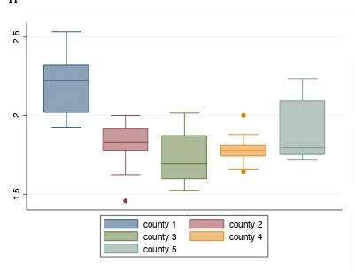
The estimates of the dependence parameter of the survival Gumbel copula (Figure A1

in Appendix) indicate a solid level of dependence of the study farm yields on the

selected drought index. For almost all study farms, the estimates of the dependence

parameter are above 1.5. However, the highest degree of dependence was estimated

for the farms in the first county, where the dependence parameter estimates are above

2.0 for the majority of the farms, while the lowest level of dependence on average was

found for the farms in county 3.

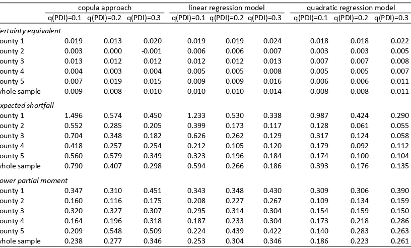
Table 1 summarizes the estimates of the risk reduction for single weather index

insurance contacts. Independent of the approach used for contract rating, as well as

the choice of the weather index threshold level, risk reduction evaluated in terms of

certainty equivalent is almost negligible. This result is not surprising considering the

independence assumption of the expected utility model, which implies that risk

preferences are linear in probabilities. Accordingly, relatively small changes in the

left tail of the outcome distribution should not have a substantial inflence on the

expected utility value. )

(15)

The estimates of risk reduction based on the expected shortfall criterion show that a

substantially higher risk reduction was found for the copula-based approach than for

the regression-based approach. On average, for the whole sample, the copula-based

insurance contract with the threshold equal to the first decile of the weather index

[image:15.595.96.504.247.493.2]

distribution would increase expected yield of the lowest 10% yield records by 79%.

Table 1. Relative risk-reduction estimates for copula-based approach and

regression-based approach (3 weather index thresholds): catastrophic years determined regression-based on

farm yield distribution

Source: author’s estimates

The corresponding values for the hypothetical insurance contacts based on the linear

and quadratic regression models are 59 and 39%, respectively. Risk reduction

reduces for contracts with higher threshold levels of the weather index. Additionally,

insurance contracts based on the linear regression model specification are found to

provide higher risk reductions than those corresponding with the quadratic model.

Consequently, in the following we reduce our discussion to the comparison of results

obtained from the copula-based insurance approach and the linear regression model.

The results of the t-test for the difference between two sample means indicate that the

copula-based weather index contracts with the threshold levels equal to q0.2(W) and

q0.3(W) would allow for a significantly higher average risk reduction (at the 5% level

of significance) than corresponding contracts derived on the basis of the linear

q(PDI)=0.1 q(PDI)=0.2 q(PDI)=0.3 q(PDI)=0.1 q(PDI)=0.2 q(PDI)=0.3 q(PDI)=0.1 q(PDI)=0.2 q(PDI)=0.3

Certainty)equivalent

county31 0.019 0.013 0.020 0.019 0.019 0.024 0.018 0.018 0.022 county32 0.003 0.000 70.001 0.006 0.006 0.007 0.003 0.003 0.005 county33 0.013 0.012 0.012 0.012 0.012 0.013 0.007 0.007 0.008 county34 0.004 0.003 0.004 0.005 0.005 0.008 0.005 0.005 0.007 county35 0.007 0.019 0.015 0.009 0.009 0.016 0.006 0.006 0.011 whole3sample 0.009 0.008 0.010 0.010 0.010 0.014 0.008 0.008 0.011

Expected)shortfall

Lower)partial)moment)

(16)

regression; for the insurance contracts with the q0.1(W) threshold the difference

between average risk reductions from two alternative approaches is not significant.

Though our estimates of the lower partial moment suggest a solid reduction in the

variability of farm yields in the left tail of the yield distribution, there are no

significant differences in the average risk reductions between the contracts based on

the copula approach and those derived by means of the linear regression model

according to the two-sample mean t-test. Obviously, because they provide higher

levels of coverage for the yield losses caused by extreme drought events, the

copula-based contracts charge higher premiums; also in the years when an extreme yield loss

was caused by another peril and thus no indemnity was paid by the specified

insurance contract. This might be an explanation for a relatively moderate

performance of copula-based insurance contracts as evaluated by using the lower

[image:16.595.99.505.420.583.2]

partial moment.

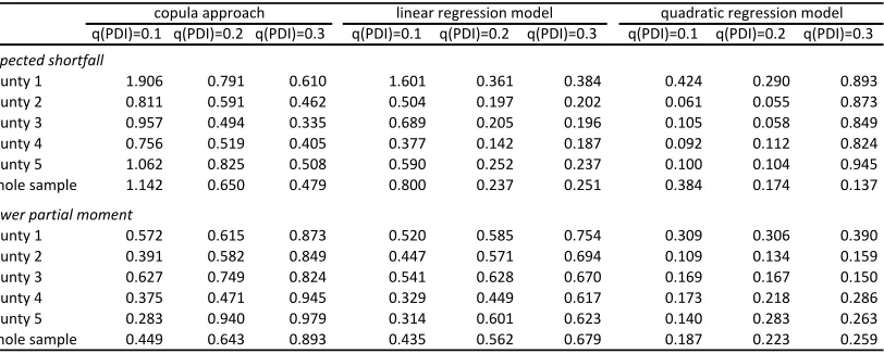
Table 2. Relative risk reduction estimates for copula-based approach and

regression-based approach (3 weather index thresholds): catastrophic years determined regression-based on

weather index distribution

An additional cause of the relatively moderate performance of the weather index

insurance contracts might be explained by the capacity of the weather index to signal

extreme drought occurrence. The estimates of risk reduction presented in Table 1 are

obtained by employing the yield unconditional distribution. In this case, left-tail

quantiles of the yield distribution may not necessarily correspond with left-tail

quintiles of the weather index. If the number of disconcording pairs of joint yield and

weather index realizations is not negligible, the evaluation of the insurance contract

q(PDI)=0.1 q(PDI)=0.2 q(PDI)=0.3 q(PDI)=0.1 q(PDI)=0.2 q(PDI)=0.3 q(PDI)=0.1 q(PDI)=0.2 q(PDI)=0.3 Expected(shortfall

county31 1.906 0.791 0.610 1.601 0.361 0.384 0.424 0.290 0.893 county32 0.811 0.591 0.462 0.504 0.197 0.202 0.061 0.055 0.873 county33 0.957 0.494 0.335 0.689 0.205 0.196 0.105 0.058 0.849 county34 0.756 0.519 0.405 0.377 0.142 0.187 0.092 0.112 0.824 county35 1.062 0.825 0.508 0.590 0.252 0.237 0.100 0.104 0.945 whole3sample 1.142 0.650 0.479 0.800 0.237 0.251 0.384 0.174 0.137 Lower(partial(moment(

(17)

effectiveness should account for this fact. In Table 2, we summarize risk reduction

estimates obtained by employing yield realizations, conditioned of the weather index

distribution quantiles. These estimates show what would be the risk reduction, if the

selected weather index would perfectly identify the occurrence of drought and there

were no other risk causing extreme yield losses. In this case, the copula-based

insurance contracts would clearly outperform the contracts derived by employing the

linear regression model. The t-test indicates that the average risk reductions due to

the copula-based contracts with the q0.2(W) and q0.3(W)-thresholds would be

significantly higher at the 1% level than the average risk reduction for equivalent

contacts based on the linear regression as measured by both criteria - expected

shortfall and lower partial moment. The difference in the average risk reduction

between two alternative approaches for the contracts with the q0.1(W) threshold is

found to be significant at the 5% level for the expected shortfall and not significant

for the lower partial moment. The highest risk reduction, in terms of an increase of

the expected shortfall, were obtainable by setting the weather index threshold to

correspond with the first quantile of its distribution, while higher reductions in the

variability of the outcome would be achieved at higher levels of the index threshold.

CONCLUSIONS

The paper presents a copula-based approach for rating weather index insurance

designed to provide coverage for yield losses due to extreme weather events. The

effectiveness of this approach is compared with the common regression-based

approach. Our preliminary results suggest that the application of the copula approach

might improve the performance of weather index insurance. However, the

identification of drought seems to be problematic. Therefore, the selection of an

adequate weather indicator to signal occurrence of an extreme event is a precondition

(18)

REFERENCES

Acharya, V., Pedersen, L. H., Philippon, T., and M. Richardson, M. (2012).

Measuring systemic risk. CEPR Discussion Papers 8824, C.E.P.R. Discussion Papers.

Akter, S., and Fatema, N. (2011). The role of microcredit and microinsurance in

coping with natural hazard risks. Contributed paper, 18th Annual Conference of the

European Association of Environmental and Resource Economists, Rome, June

29-July 2, 2011, Rome.

Barnett, B., and Mahul, O. (2007). Weather Index Insurance for Agriculture and Rural

Areas in Lower-Income Countries. Am. J. Agr. Econ.89 (5): 1241-1247.

Bokusheva, R. (2011). Measuring dependence in joint distributions of yield and

weather variables. Agricultural Finance Review, 71:120-141.

Bokusheva, R., and Breustedt, G. (2012). The effectiveness of weather-based index

insurance and area-yield crop insurance: How reliable are ex post predictions for yield

risk reduction? Quarterly Journal of International Agriculture, 51 (2):135-9156.

Breustedt, G., R. Bokusheva, R., and O. Heidelbach, O. (2008): The potential of index

insurance schemes to reduce farmers’ yield risk in an arid region. Journal of

Agricultural Economics 59 (2): 312-328.

Cole, S., X. Giné, X., J. Tobacman, J., P. Topalova, P., R. Townsend, R., and J.

Vickery, J. (2013). Barriers to Household Risk Management: Evidence from India.

American Economic Journal: Applied Economics, 5 (1): 104-35.

Gamerman, D., and Lopes, H.F. (2006). Markov Chain Monte Carlo: Stochastic

Simulation for Bayesian Inference, 2nd ed. Chapman & Hall, London: Chapman &

Hall.

Genest, C., B. Remillard, B., and D. Beaudoin, D. (2009). Goodness-of-fit tests for

copulas: A review and a power study. Insurance: Mathematics and Economics, 44:

199-214.

Hardaker J.B., Huirne, R.B.M., Anderson, J.R., and Lien, G. (2007). Coping with risk

in agriculture. 2nd edition. Wallingford: CABI Pub, Wallingford.

Mainik, G., and Schaanning, E., (2012). On dependence consistency of CoVaR and

some other systemic risk measures. RiskLab, Department of Mathematics, ETH

(19)

McNeil A., Frey R., and Embrechts, P. (2005). Quantitative Risk Management.

Princeton: Princeton University Press, Princeton, 2005.

Mobarak, A.M., and Rosenzweig, M. (2012). Selling Formal Insurance to the

Informally Insured. Yale University Economic Growth Center Discussion Paper No.

1007.

Nelsen, R. B. (1999). An Introduction to Copulas. Springer, New York: Springer.

Norton, M., Holthaus, E., Madajewicz, M., Osgood, D., Peterson, N., Mengesha

Gebremichael, C., Mullally, C., and Teh, T.L. (2011). Investigating Demand for

Weather Index Insurance: Experimental Evidence from Ethiopia. Selected Paper

prepared for presentation at the Agricultural & Applied Economics Association’s

2011 AAEA & NAREA Joint Annual Meeting, Pittsburgh, Pennsylvania, July 24-26

July.

Skees, J.R., Black, J.R., and Barnett, B.J. Barnett (1997). Designing and Rating an

Area Yield Crop Insurance Contract. American Journal of Agricultural Economics,

79: 430-438.

Skees, J., Murphy, A., Collier, B., McCord, M.J., and Roth, J. (2007). Scaling Up

Index Insurance, What is needed for the next big step forward? Microinsurance

Centre, LLC, Global Ag Risk, Inc.

Sklar, A. 1959. Fonctions de répartition à n dimension et leurs marges, Publ. Inst.

Stat. Univ. Paris, 1959; 8:299-231.

Vedenov, D.V. and Barnett, B.J. Barnett (2004). Efficiency of weather derivatives as

primary crop insurance instruments. In: Journal of Agricultural and Resource

Economics 29 (3): 387-403.

Wang, H. H., R. N. Karuaihe, R., Young, D. L., Young and Y. Zhang, Y. (2013).

Farmers’ demand for weather-based crop insurance contracts: the case of maize in

South Africa. Agrekon 52(1): 87-110.

(20)

Appendix

[image:20.595.89.490.83.389.2]

Figure A1. Estimates of survival Gumbel copula dependence parameter

1.5

2

2.5

county 1 county 2

county 3 county 4